Prediction of Mass Transfer Time Relaxation Parameter for Boiling Simulation on the Shell-Side of LNG Spiral Wound Heat Exchanger

Abstract

The objective of this present study is to propose an approach to predict mass transfer time relaxation parameter for boiling simulation on the shell-side of LNG spiral wound heat exchanger (SWHE). The numerical model for the shell-side of LNG SWHE was established. For propane and ethane, a predicted value of mass transfer time relaxation parameter was presented through the equivalent evaporation simulations and was validated by the Chisholm void fraction correlation recommended under various testing conditions. In addition, heat transfer deviations between simulations using the predicted value of mass transfer time relaxation parameter and experiments from Aunan were investigated. The boiling characteristics of SWHE shell-side were also visualized based on the simulations with VOF model. The method of predicting mass transfer time relaxation parameter may be well applicable to various phase change simulations.

1. Introduction

Spiral wound heat exchanger (SWHE) has been used as main cryogenic heat exchanger in most of liquefied natural gas (LNG) production plants. Use of SWHE in LNG plants is based on the advantages of multistream capability, high compactness, efficient heat transfer, sufficient flexibility with regard to a broad temperature and pressure range, better robustness for single phase, and two-phase flow.

A principle sketch of a multistream SWHE is depicted in Figure 1. Large amounts of small-diameter tubes are coiled in layers around a core cylinder. The coiling direction alternates from one layer to the next. The distances between successive layers are held constant by space bars. The tubes are connected to tube sheets and collected in headers at both ends of the heat exchanger. Natural gas and alkane refrigerant vapor constituting different streams are routed in upward flow in the tube-side of SWHE. The natural gas stream is precooled and subsequently liquefied and subcooled. The refrigerant vapor stream is liquefied and subcooled and then leaves from the heat exchanger. After being throttled, the hydrocarbon refrigerant boils in downward flow on the shell-side and finally returns to the refrigerating compressor.

Figure 1:

A principal sketch of a multistream SWHE.

Technologies of SWHE have been proprietary for very few manufacturers, such as Air Products and Chemicals Incorporation in USA, Linde Group in Germany, and Statoil ASA in Norway. To achieve optimal design and evaluate heat transfer performance of SWHE, theoretical and experimental studies should be done deeply.

In the scope of SWHE shell-side, fewer literatures have been reported until now. One of the most important features of SWHE shell-side geometry is the flow gap width. The gap width is used to calculate the flow area and the mass velocity. The simplest approach to finding the gap width is to calculate the minimum or maximum radial distance between two tube layers. The real distance, however, lies between the in-line and the staggered configurations. Therefore, an average distance can be found by integration between these two arrays. This work had been done by Glaser [1], Gilli [2], and Smith [3]. Barbe et al. [4] proposed a method for heat transfer coefficient and friction pressure drop calculation through semiempirical theories. The method is applicable to two-phase flow within the shell and the conclusions are testified by their experimental data with air-water mixture and propane fluids. Abadzic [5] compared several existing heat transfer correlations with published measurements and presented a correlation used in all sorts of fluids in the form of single phase flow. Fredheim [6] and Aunan [7] investigated the heat transfer and friction pressure drop of pure alkanes (C1, C2, and C3) and mixtures (C1/C2, C2/C3) on the shell-side of SWHE model in a test facility. They pointed out consistently that different flow regimes are usually present on the shell-side, and introduced three different flows on shell-side: film, shear, and superheated flows. Various correlations for single and two-phase heat transfer and frictional pressure drop were validated. According to the experimental data, Neeraas et al. [8, 9] recommended the optimum heat transfer and friction pressure drop correlations, respectively, for gas and film flows. The calculated and measured values accorded well.

In contrast to experiment investigations, CFD study of boiling flow on the shell-side of LNG SWHE has not been carried out. The reasons have been possibly out of CFD model imperfection in two-phase flow and the bulky and complicated geometry of SWHE causing a large number of computational cells. Even though there are many simulation difficulties, it is worthy to apply CFD technologies to LNG SWHE for saving experimental costs. Solving mass transfer is a key step on the shell-side two-phase flow as far as heat transfer and pressure drop are concerned. While ANSYS FLUENT software is focused on the simulations for shell stream, mass transfer time relaxation parameter must be confronted and determined during the use of evaporation and condensation model. According to the works of Lee [10] and Wu et al. [11], the value of the parameter could be set uniformly equal to 0.1 s⁻¹, though the different physical problems were dealt with in various working fluids. However, Yang et al. [12] specified the value to 100 s⁻¹ in a case similar to Wu et al.'s [11] working condition. In the above studies, the determination of mass transfer time relaxation parameter is not elaborated in detail and is not guided to other boiling problems. The purpose of this paper is to present a calculation method of mass transfer time relaxation parameter for refrigerating fluid which vaporizes on the shell-side of LNG SWHE and to provide reference for other phase change simulations using evaporation-condensation model.

2. CFD Model

2.1. Geometric Configuration and Boundaries

To realize precise simulations, a mass of meshes are necessary. Subject to computational grid number, one-tenth of the 3D geometry (based on the tested SWHE model in Aunan [7]) is cut and is finally adopted after assuming the symmetry of 3D geometry about the Z-axis in the course of shell-side flow. The computational domain and boundaries are illustrated in Figure 2. And in the numerical simulations, the same geometrical data (from the tested SWHE model in Aunan [7]) are also used in order to compare the deviations between numerical results and experimental measurements.

Figure 2:

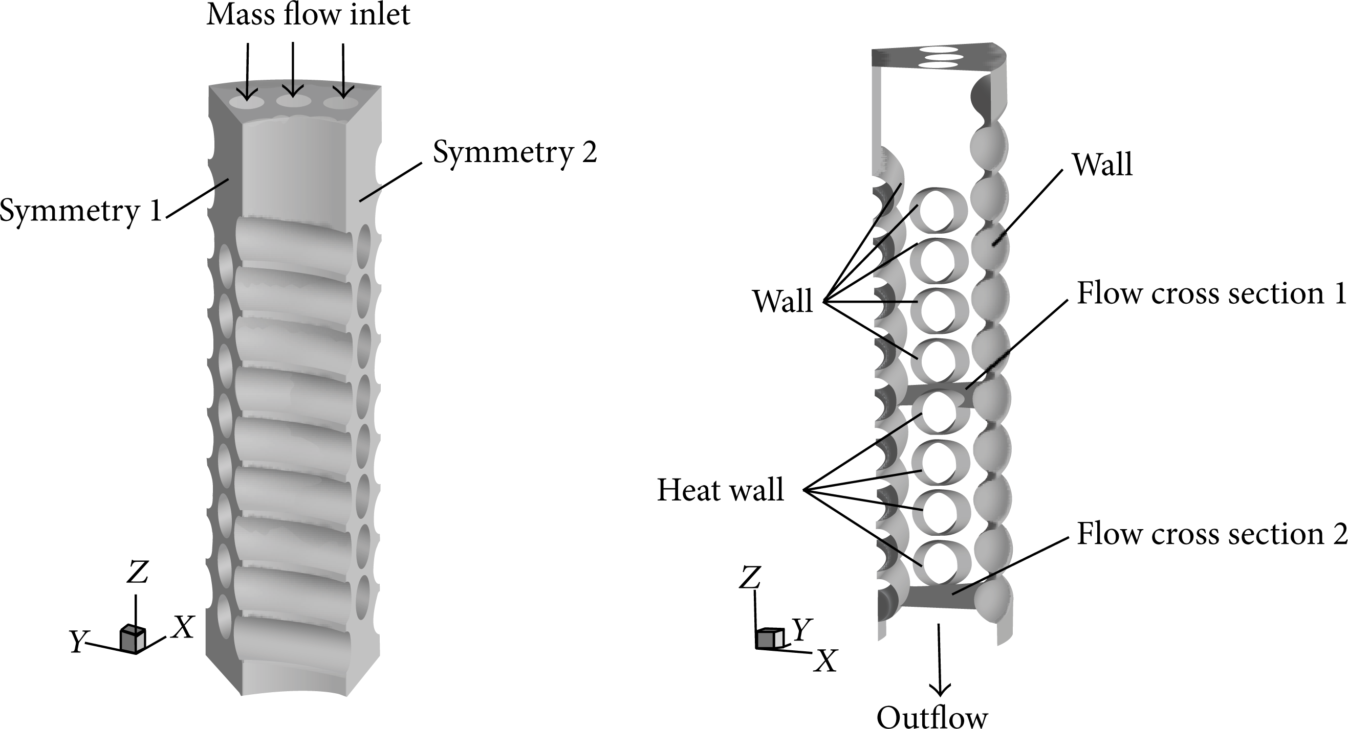
A schematic map of geometrical configuration and boundaries.

The model consists of one interlayer coil containing eight parallel tubes and two half-tube coils treated as the inner and outer walls. The cryogenic refrigerant flows down from three inlets whose diameters are 10 mm on the top plane and flows out from the bottom plane. The upper four tubes in the central coil are adiabatic for flow stabilization, and the lower four are heated by a constant heat flux in order to obtain the heat transfer coefficient of two-phase flow. Flow cross sections 1 and 2 have the same flow areas and are designated for data processing. The axial sections on both sides of the model are handled, respectively, as symmetry boundaries 1 and 2.

Through ANSYS ICEM CFD 14.0, the model is meshed by unstructured grids. Firstly, the boundaries are dealt as different mesh parts, the mesh max size is determined by the axial tube gap of coils, and a thinner boundary layer is set over the walls of three layer coils; the initial height, the height ratio, and the number of layers are 0.005 mm, 1.2, and 10, respectively; secondly, the computational domain of the model is meshed by Tetra/Mixed cells. To select the appropriate grid and testify the grid independency, three mesh schemes are performed, which are shown in Table 1.

Table 1:

Three kinds of mesh schemes of the CFD model.

Mesh method	Mesh max size ofaxial tube gap of coils(mm)	Mesh max size ofother boundaries(mm)	Cell quantities
1	0.6	1.2	1400644
2	0.7	1.4	1124309
3	0.8	1.6	836713

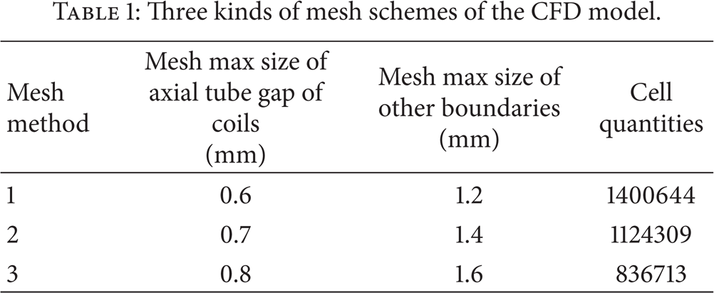
The simulations of superheated vapor flow with methane are carried out to verify the three mesh methods. The comparisons between the simulation results and the corresponding measurements are presented in Table 2, which show that the quantity of cells reaching 1124309 gives the satisfactory balance between computational accuracy and cell quantities. So in this paper, the mesh method 2 is chosen for the simulation.

Table 2:

The simulation deviations of superheated vapor flow with methane for different mesh schemes.

Mesh method	Heat transfer coefficient deviation(%)	Friction pressure drop gradient deviation(%)
1	−17.25	−18.37
2	−17.52	−20.71
3	−17.80	−21.32

2.2. Governing Equations

In this study, the volume of fluid (VOF) model in ANSYS FLUENT 14.0 is used to simulate boiling flow on the shell-side of SWHE. As to VOF model, volume fraction of each phase in a computational cell is solved, and the information on phase distribution can be consequently extracted from the volume fraction. In each cell, the summation of each phase's volume fraction is unity.

Tracking interface between phases is accomplished by solving continuity equations for the volume fractions of one or more phases. For the vapor-liquid flow, the equations are

$\begin{array}{c}\frac{\partial {\alpha }_V}{\partial t}+\nabla ·\left({\alpha }_V\overrightarrow{v}\right)=\frac{S_m}{{\rho }_V},\\ \frac{\partial {\alpha }_L}{\partial t}+\nabla ·\left({\alpha }_L\overrightarrow{v}\right)=-\frac{S_m}{{\rho }_L},\end{array}$

(1)

where S _m is the mass source term and represents the mass transfer due to phase change.

A single momentum equation for an incompressible flow is solved throughout the domain, and the resulting velocity field is shared among the phases. The momentum equation is represented as

$\frac{\partial }{\partial t}\left(\rho \overrightarrow{v}\right)+\nabla ·\left(\rho \overrightarrow{v}\overrightarrow{v}\right)=-\nabla p+\nabla ·\left[\mu \left(\nabla \overrightarrow{v}+\nabla \overrightarrow{v}{}^T\right)\right]+\rho \overrightarrow{g}+\overrightarrow{F},$

(2)

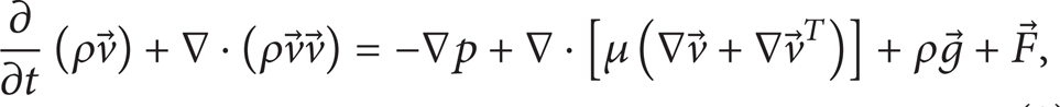
where $\overrightarrow{F}$ is volumetric force and here is the surface tension force per unit volume.

In (2), ρ and μ are, respectively, treated as volume-fraction-averaged variables on the following form:

$\begin{array}{c}\rho ={\alpha }_L{\rho }_L+{\alpha }_V{\rho }_V,\\ \mu ={\alpha }_L{\mu }_L+{\alpha }_V{\mu }_V.\end{array}$

(3)

All other material properties such as thermal conductivity are computed in the same manner. Therefore, the properties in each cell depend on the volume fraction and become different.

The energy equation, also shared among the phases, is shown here:

$\frac{\partial }{\partial t}\left(\rho E\right)+\nabla ·\left[\overrightarrow{v}\left(\rho E+p\right)\right]=\nabla ·\left({\lambda }_{\text{eff}}\nabla T\right)+S_e.$

(4)

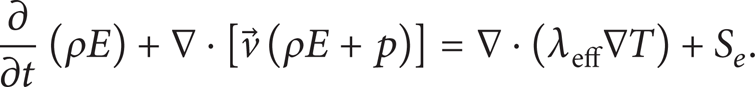
The VOF model treats the energy, E, as mass-averaged variable:

$E=\frac{{\alpha }_L{\rho }_L{E}_L+{\alpha }_V{\rho }_V{E}_V}{{\alpha }_L{\rho }_L+{\alpha }_V{\rho }_V},$

(5)

where E _L and E _V are based on the specific heat of single phase as well as the shared temperature. The energy source term, S _e , is the volumetric heat source. In the present study, this source term S _e is modeled to simulate heat transfer during boiling.

2.3. Modeling of Source Terms

2.3.1. Mass Source Term

A mass transfer model concerning the process of evaporating and condensing introduced by Lee [10] is adopted in VOF module. In the module, mass transfer mainly depends on the shared temperature and the saturate temperature. The direction and magnitude of mass transfer are described as follows.

If T ≥ T _sat , the evaporation occurs. The mass of the liquid phase in the control volume decreases, and the mass of vapor phase increases correspondingly, which means the mass is transferred from the liquid phase to the vapor phase. The mass transfer rate is

$S_m=\beta {\alpha }_L{\rho }_L\frac{T-T_{\mathrm{sat}}}{T_{\mathrm{sat}}}.$

(6)

In ANSYS FLUENT, positive mass transfer is defined as being from the liquid phase to the vapor phase for evaporation-condensation problems.

If T < T _sat , the condensation occurs. The mass of the liquid phase in the control volume increases, and the mass of vapor phase decreases correspondingly, which means the mass is transferred from the vapor phase to the liquid phase. The mass transfer rate is

$S_m=\beta {\alpha }_V{\rho }_V\frac{T-T_{\mathrm{sat}}}{T_{\mathrm{sat}}},$

(7)

where β is the mass transfer time relaxation parameter and is the research focus in this paper. To various alkane fluids, a different value of the parameter should be acquired for the right evaporation on the shell-side of SWHE.

2.3.2. Heat Source Term

Heat transfer is simply deduced from the evaporation or condensation. As long as mass transfer is obtained, heat transfer can be directly determined as

$S_e=-h_{\mathrm{LH}}{S}_m,$

(8)

where h _LH is the latent heat.

2.4. Solution and Discretization Method

The fluids are assumed to be incompressible and to have constant fluid properties. Transient simulations are carried out with the first order implicit scheme of transient term, and the explicit geometric reconstruction scheme also is selected for interface between vapor and liquid phases. In light of improvements on streamline curvature, the RNG k-ε turbulent model is adopted with the enhanced wall treatment. The PISO pressure-velocity coupling scheme is employed for neighbor correction and skewness correction. The second order upwind differencing scheme is implemented for solving the momentum, turbulent kinetic energy, and turbulent dissipation rate equations. Pressure discretization is the PRESTO scheme, and the evaluation of spatial gradients is based on the Green-Gauss theorem. An optional surface tension force model is taken into account with regard to phase interaction. All simulations are performed on computer servers with 12 cores/24 threads and 2.4 GHz processors. The time step size is set by 10⁻⁵ s in order to keep the Courant number meeting the requirement.

3. An Approach to Predict β

Referring to (6) and (7), mass transfer will change as long as β value varies; consequently, the shared temperature should be modified, as it will lead to differential effects on both evaporation and heat transfer.

For ANSYS FLUENT, vapor volume fraction is widely used rather than vapor quality and visualizes the mass transfer. For boiling flow simulations, if the different β values are set, the vapor volume fractions in the surface of outlet are distinguishing.

For the above reasons, some simulations with different β values are carried out under a certain condition. Based on a comparison of vapor volume fraction, the equivalent-evaporation simulation (EES) is implemented to predict β value.

The EES is the case that a vapor quality (x) at inlet is determined by the value derived from (9) along with no heat-mass transfer during shell stream. Because of no heat input and β being zero, the energy equation is not solved. Consider

$x=\frac{m_{V,\text{in}}+Q/h_{\mathrm{LH}}}{m_{V,\text{in}}+m_{L,\text{in}}},$

(9)

where m_{V, in} and m_{L, in} represent the vapor and liquid mass flow rates at the SWHE inlet, respectively; Q stands for the heat input in the model. The values for both mass flow rate and heat input are dependent on the experimental data [7].

According to the different β values in the simulations, the corresponding vapor volume fractions in the flow cross section 2 which represent different evaporating levels are compared with that stemmed from the EES so that the parameter value is preliminarily available. Additionally, heat transfer deviations between the simulations and experiment result are considered as an additional condition to predict β value.

To ensure the prediction accuracy, void fraction correlation is also put into use to verify the validity of β value. Usually in CFD software, the vapor volume fraction in a surface equals approximately the void fraction; therefore, in cross section 2, the vapor volume fraction in the simulation results may be contrasted to the void fraction computed from a void fraction correlation. A void fraction correlation which is suitable for SWHE shell-side flow cannot be found in the open literatures; however, some related correlations have to be brought into the comparison. When there is a correlation which takes void fraction close to the vapor volume fraction gained from both the simulations using the preliminary β value and the corresponding EES under various conditions, not only the β value is confirmed to be appropriate, but also the recommended correlation for the shell-side of SWHE will be found.

3.1. Simulation Range and Conditions

In ANSYS FLUENT, the default β value is 0.1 s⁻¹. The simulation range of β value is confined to some certain values including 0.1, 1, 2, 3, 4, and 5 s⁻¹, after trial simulations are performed and analyzed.

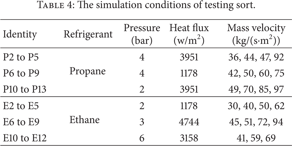
The simulation conditions are classified into two kinds: one is the solution sort which is used to predict β value and is shown in Table 3 and the other is the testing sort which is adopted to validate β value under different circumstances and is shown in Table 4. All conditions are in agreement with those in Aunan's experiments [7]. The tested fluids include propane and ethane, and vapor quality at inlet is zero in the simulations except the respective EESs.

Table 3:

The simulation conditions of solution sort.

Identity	Refrigerant	Pressure(bar)	Heat flux(w/m2)	Mass velocity(kg/(s·m2))
P1	Propane	4	3966	82
E1	Ethane	6	3237	59

Table 4:

The simulation conditions of testing sort.

Identity	Refrigerant	Pressure(bar)	Heat flux(w/m2)	Mass velocity(kg/(s·m2))
P2 to P5	Propane	4	3951	36, 44, 47, 92
P6 to P9		4	1178	42, 50, 60, 75
P10 to P13		2	3951	49, 70, 85, 97
E2 to E5	Ethane	2	1178	30, 40, 50, 62
E6 to E9		3	4744	45, 51, 72, 94
E10 to E12		6	3158	41, 59, 69

3.2. Void Fraction Correlations

The void fraction in cross section 2 is calculated by some correlations which are shown in Table 5. These correlations are generally mentioned in some literatures of two-phase flow and are mostly suitable for tube bundles. When the correlations are applied, the involved vapor quality in cross section 2 is also gained from (9).

Table 5:

The summary of void fraction correlations selected.

Identity	Authors	Correlation	Scope of application
VFC1	Chisholm [13]	$\mathrm{\epsilon }=\frac{\mathrm{1}}{\mathrm{1}+s\left({\mathrm{\rho }}_V/{\mathrm{\rho }}_L\right)\left(\left(\mathrm{1}-x\right)/x\right)}$ ;  $s={\left[\mathrm{1}+x\frac{\left({\mathrm{\rho }}_L-{\mathrm{\rho }}_V\right)}{{\mathrm{\rho }}_V}\right]}^{\mathrm{1}/\mathrm{2}}$	Evaporation in tube and channel
VFC2	Speddig and Spence [14]	$\mathrm{\epsilon }=\frac{\mathrm{1}}{\mathrm{1}+\mathrm{2.22}{\left(\mathrm{1}-x/x\right)}^{\mathrm{0.65}}{\left({\mathrm{\rho }}_V/{\mathrm{\rho }}_L\right)}^{\mathrm{0.65}}}$	Horizontal and vertical stratified flow in tube
VFC3	Ishihara et al. [15]	$\mathrm{\epsilon }=\mathrm{1}-\frac{\mathrm{1}}{{\mathrm{\varphi }}_L}$ ;  ${\mathrm{\varphi }}_L=\mathrm{1}+\frac{\mathrm{8}}{{\mathrm{\chi }}_{\text{tt}}}+\frac{\mathrm{1}}{{{\mathrm{\chi }}_{\text{tt}}}^{\mathrm{2}}}$ ; ${\mathrm{\chi }}_{\text{tt}}=\frac{\mathrm{1}-x}{x}{\left(\frac{{\mathrm{\rho }}_V}{{\mathrm{\rho }}_L}\right)}^{\mathrm{0.57}}{\left(\frac{{\mathrm{\mu }}_L}{{\mathrm{\mu }}_V}\right)}^{\mathrm{0.11}}$	Vertical flow on tube bundles, χtt < 0.2
VFC4	Dowlati et al. [16]	$\mathrm{\epsilon }=\mathrm{1}-{\left(\mathrm{1}+\mathrm{35}{j_V}^{\mathrm{*}}+\mathrm{50}{j_V}^{\mathrm{*}}\right)}^{-\mathrm{1}/\mathrm{2}}$ ;   ${j_V}^{\mathrm{*}}=\frac{Gx}{\sqrt{g{\mathrm{\rho }}_{V}D({\mathrm{\rho }}_L-{\mathrm{\rho }}_V)}}$	Vertical flow across a horizontal tube bundle
VFC5	Fair and Klip [17]	$\mathrm{\epsilon }=\mathrm{1}-{\left(\frac{\mathrm{1}}{{\mathrm{\varphi }}_L}\right)}^{\mathrm{0.5}}$ ;  ${\mathrm{\varphi }}_L=\mathrm{1}+\frac{\mathrm{20}}{{\mathrm{\chi }}_{\text{tt}}}+\frac{\mathrm{1}}{{{\mathrm{\chi }}_{\text{tt}}}^{\mathrm{2}}}$ ; ${\mathrm{\chi }}_{\text{tt}}=\frac{\mathrm{1}-x}{x}{\left(\frac{{\mathrm{\rho }}_V}{{\mathrm{\rho }}_L}\right)}^{\mathrm{0.57}}{\left(\frac{{\mathrm{\mu }}_L}{{\mathrm{\mu }}_V}\right)}^{\mathrm{0.11}}$	Vertical flow across a horizontal bundle
VFC6	Bankoff [18]	$\mathrm{\epsilon }=\frac{\mathrm{0.71}+\mathrm{0.0145}p}{\mathrm{1}+\left(\left(\mathrm{1}-x\right){\mathrm{\rho }}_V/x{\mathrm{\rho }}_L\right)}$  (p in MPa)	Vertical flow in conduit
VFC7	Zivi [19]	$\mathrm{\epsilon }=\frac{\mathrm{1}}{\mathrm{1}+(\left(\mathrm{1}-x\right)/x){\left({\mathrm{\rho }}_V/{\mathrm{\rho }}_L\right)}^{\mathrm{2}/\mathrm{3}}}$	The idealized steady-state annular flow
VFC8	Schrage et al. [20]	$\mathrm{\epsilon }=\frac{\mathrm{1}+\mathrm{0.123}\text{F}{{\text{r}}_L}^{-\mathrm{0.191}}\ln x}{\mathrm{1}+\left(\left(\mathrm{1}-x\right)/x\right)\left({\mathrm{\rho }}_V/{\mathrm{\rho }}_L\right)}$ ;  $\text{F}{\text{r}}_L=\frac{G}{{\mathrm{\rho }}_L{\left(gD\right)}^{\mathrm{1}/\mathrm{2}}}$	Vertical flow across a horizontal tube bundle
VFC9	Wallis [21]	$\mathrm{\epsilon }={\left(\mathrm{1}+{\mathrm{\chi }}^{\mathrm{0.8}}\right)}^{-\mathrm{0.378}}$ ;  ${\mathrm{\chi }}_{\text{tt}}={\left(\frac{\mathrm{1}-x}{x}\right)}^{\mathrm{0.9}}{\left(\frac{{\mathrm{\rho }}_V}{{\mathrm{\rho }}_L}\right)}^{\mathrm{0.5}}{\left(\frac{{\mathrm{\mu }}_L}{{\mathrm{\mu }}_V}\right)}^{\mathrm{0.1}}$	General correlation
VFC10	Domanski and Didion [22]	ε = 0.823 − 0.157ln⁡χtt;  ${\mathrm{\chi }}_{\text{tt}}={\left(\frac{\mathrm{1}-x}{x}\right)}^{\mathrm{0.9}}{\left(\frac{{\mathrm{\rho }}_V}{{\mathrm{\rho }}_L}\right)}^{\mathrm{0.5}}{\left(\frac{{\mathrm{\mu }}_L}{{\mathrm{\mu }}_V}\right)}^{\mathrm{0.1}}$	General correlation, 10 < χtt < 189
VFC11	Xu et al. [23]	$\mathrm{\epsilon }=\frac{\mathrm{3.7}\text{F}{{\text{r}}_L}^{\mathrm{0.11}}{{\mathrm{\chi }}_{\text{tt}}}^{-\mathrm{0.446}}}{\mathrm{1}+\mathrm{3.7}\text{F}{{\text{r}}_L}^{\mathrm{0.11}}{{\mathrm{\chi }}_{\text{tt}}}^{-\mathrm{0.446}}}$ ;  $\text{F}{\text{r}}_L=\frac{G^{\mathrm{2}}}{{{\mathrm{\rho }}_L}^{\mathrm{2}}gD}$	Down-flow across a horizontal tube bundle

4. Result and Discussion

4.1. Predicting the Value of β

Firstly, the comparison of vapor volume fraction between simulations under different β values and the EES is shown in Figure 3. It can be clearly seen that, for propane, when β = 3 s⁻¹, the simulated vapor volume fraction in cross section 2 approaches that in the EES. And for ethane, the deviation is produced when β = 4 s⁻¹ smaller than that when β = 3 s⁻¹. Then, heat transfer deviations between the simulation results under β = 2, 3, 4 s⁻¹ and the corresponding experiments from Aunan [7] are shown in Figure 4. It indicates that, for ethane, there exists the minimum heat transfer deviation between the simulation result using β = 3 s⁻¹ and the corresponding experiment result from Aunan [7]. So the predicted β value is treated uniformly as 3 s⁻¹ for propane and ethane. This value will be further evaluated in the simulations of testing sort.

Figure 3:

The comparison of vapor volume fraction between the simulation results under different β values and the EES.

Figure 4:

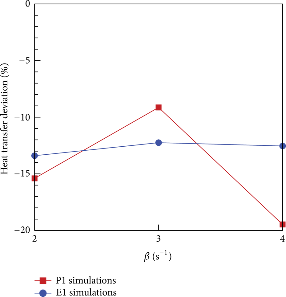
Heat transfer deviation between the simulation results under β = 2, 3, 4 s⁻¹ and the corresponding experiment results from Aunan [7].

4.2. Filtrating Void Fraction Correlations

Because the void fraction correlation which may be applicable to the shell-side flow of SWHE is not found; eleven correlations are employed to contrast the void fractions to the vapor volume fraction of the EES in P1 and E1 conditions so that a correlation might be screened out to verify the predicted β value in testing conditions. The comparison results between void fractions from the correlations and vapor volume fraction from the EES are listed in Table 6. It is found that the correlations from VFC1 to VFC5 provide the acceptable deviations in the P1 and E1 conditions. These five correlations are thought as the filtrated objects and will be checked under various testing conditions until a reasonable correlation is recommended for computing the void fraction on the shell-side flow of SWHE.

Table 6:

The comparison results between void fractions from the correlations and vapor volume fraction from the EES.

Simulation condition	Correlationidentity	Void fraction	Deviation %(εEES = 0.1201)	Simulation condition	Correlationidentity	Void fraction	Deviation %(εEES = 0.0998)
P1	VFC1	0.1142	−4.91	E1	VFC1	0.0899	−9.92
	VFC2	0.1103	−8.16		VFC2	0.0935	−6.31
	VFC3	0.1208	0.58		VFC3	0.1081	8.32
	VFC4	0.1290	7.41		VFC4	0.0946	−5.21
	VFC5	0.1371	14.15		VFC5	0.1238	24.05
	VFC6	0.0864	−28.06		VFC6	0.0675	−32.36
	VFC7	0.0338	−71.86		VFC7	0.0284	−71.54
	VFC8	0.0177	−85.26		VFC8	0.0103	−89.68
	VFC9	0.3190	165.61		VFC9	0.3092	209.82
	VFC10	0.2396	99.50		VFC10	0.2226	123.05
	VFC11	0.3776	214.40		VFC11	0.3543	255.01

4.3. Recommending Void Fraction Correlation

In light of the filtrated correlations from VFC1 to VFC5, void fractions are computed in all testing conditions and the comparison results are shown in Figure 5. It can be seen that there is not a correlation keeping consistent well with the respective EES in all testing conditions. In general, for propane and ethane, the Chisholm correlation (VFC1) brings the deviation to the minimum value than others after the residual sum of square between each correlation and the corresponding EES is analyzed individually.

Figure 5:

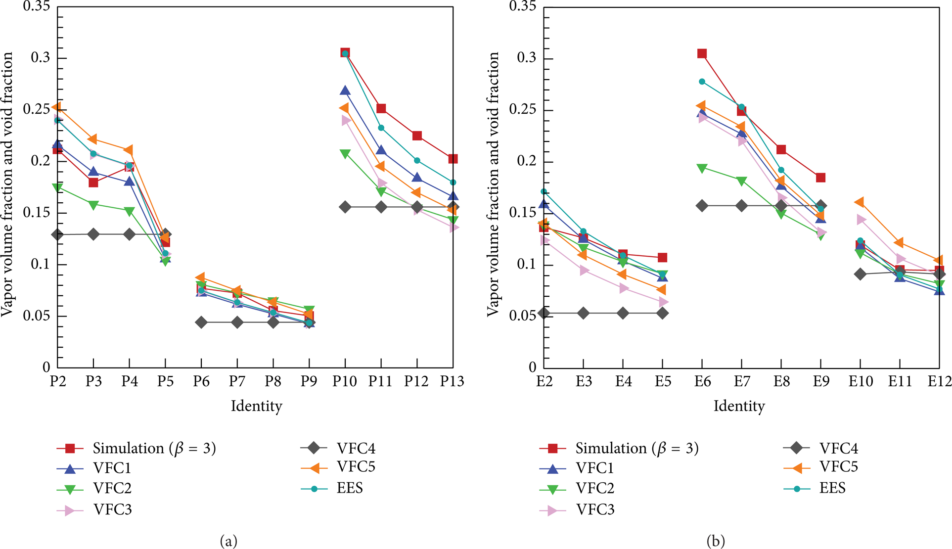
The simulated vapor volume fraction under β = 3 s⁻¹ contrast to that of the corresponding EES and contrast to the void fractions of correlations: (a) propane and (b) ethane.

Based on vapor volume fraction of the EES, the void fraction deviation between the Chisholm correlation and the corresponding EES is plotted in Figure 6. It is found that a better agreement is achieved. Therefore, the Chisholm correlation is recommended for alkane flow on the shell-side of SWHE, and it will be also used to validate β value. It is also seen from Figure 6 that, at high pressure, large mass velocity may be benefit to reduce the deviation, and these two states can exist in the actual LNG SWHE.

Figure 6:

The deviation between void fraction of the Chisholm correlation and vapor volume fraction of the corresponding EES: (a) propane and (b) ethane.

4.4. Validating the Predicted Value of β

In Figure 5, it illustrates that the simulated vapor volume fractions under β = 3 s⁻¹ are close to those of the corresponding EESs in various testing conditions for propane and ethane, and the vapor volume fraction deviations between them are displayed in Figure 7. The deviations are based on those of the corresponding EESs and are mostly within ± 20% except the conditions of E2 and E12. The deviations between the simulation results and the Chisholm correlation are also shown in Figure 7. It is found that most deviations are among ± 25% except the conditions of E9 and E12. Two kinds of deviations have the same change trend for propane and ethane, and all values of deviations can be acceptable.

Figure 7:

Vapor volume fraction deviation between simulation under β = 3 s⁻¹ and the corresponding EES, the Chisholm correlation: (a) propane and (b) ethane.

Meanwhile, heat transfer deviations between the simulations under β = 3 s⁻¹ and the corresponding experiments from Aunan [7] are examined, as shown in Figure 8. The deviations fall within −20∼10% whether propane or ethane, which means that the simulation results approach the shell-side experiment results well.

Figure 8:

Heat transfer deviation between simulations under β = 3 s⁻¹ and the corresponding experiments from Aunan [7]: (a) propane and (b) ethane.

Therefore, based on three points of vapor volume fraction, void fraction, and heat transfer, the predicted β value equal to 3 s⁻¹ is appropriate for both propane and ethane.

Additionally, with reference to Table 4, it is seen from Figure 5(a) that vapor volume fraction has the same change trend as heat flux and is opposite to the mass velocity as well as pressure, as can be affirmed from theoretical analyses. And from Figure 5(b), it denotes that heat flux is dominant factor rather than mass velocity and pressure as far as vapor volume fraction is concerned in the course of boiling flow.

4.5. Visualizing Boiling Flow on the Shell-Side of SWHE

Under different β values, the simulation pictures of boiling flows on the shell-side of SWHE are shown in Figure 9. Three important positions are considered: the interlayer coil which has four heated tube below, the axial section which is cut from the model, and the circumferential section of flow channel nearby the inner wall. It is obvious that evaporation is proportional to β value under a certain condition. Because wall adhesion option in ANSYS FUENT is used, all walls are at wetting situation, and the vapor exists mainly in the inner and outer flow channels of SWHE model. After the vapor volume fraction deviation and the heat transfer deviation which are between simulations and experiments under testing sort conditions are considered, the simulating pictures under β = 3 s⁻¹ are held to be close to the actual boiling flows for propane and ethane and will need to be confirmed further by experiments in future.

Figure 9:

The visualization of boiling flow on the shell-side of SWHE model.

5. Conclusions

In this study, it proposes an approach to predict the mass transfer time relaxation parameter for evaporation-condensation model in ANSYS FLUENT. The numerical model for boiling on the shell-side of LNG SWHE is established, and the mass and energy transfers during phase change are considered in VOF method. The important conclusions are drawn as follows.

1. After heat input is absorbed, the vapor volume fraction at outlet of a simulation using an appropriate value of mass transfer time relaxation parameter (β) is close to that one of the equivalent-evaporation simulation (EES); thus the EES can be employed to predict the β value. For propane and ethane, the respective β values used in boiling simulations are predicted to be 3 s⁻¹ uniformly through the corresponding EES cases.

2. From the point of an equivalent vapor quality, void fraction correlation which makes use of the quality at outlet of SWHE model may also validate the predicted β value. Under various simulation conditions, the void fractions computed from some correlations are compared with the vapor volume fraction of the relevant EES; then Chisholm correlation is recommended for boiling flows on the shell-side of SWHE. And the deviations between the vapor volume fractions of simulations under β = 3 s⁻¹ condition and the corresponding void fractions calculated from the Chisholm correlation are within ± 25% except two conditions (E9, E12), which denotes that the predicted β value equal to 3 s⁻¹ is appropriate.

3. Heat transfer will change when evaporation which is caused by β value varies during the course of simulations. Therefore, heat transfer deviations between simulations under β = 3 s⁻¹ condition and the corresponding experiments help further to testify the validity of β value. All deviations fall into the range from −20% to 10% and are accepted well.

It is difficult to determinate the value of mass transfer time relaxation parameter in phase change simulations, because the value is not obtained from experiments and theoretical derivation until now. However, an approach to predict the value by comparing the vapor volume fractions of simulations under different β values with that one of the relevant EES and with the void fraction derived from a recommended correlation is instructive as well as feasible. The method may be applicable to the different fluids and all kinds of phase change problems, and β value can be utilized in numerical simulations.