Numerical Investigation of Viscous Flow Velocity Field around a Marine Cavitating Propeller

Abstract

Velocity field around a ship cavitating propeller is investigated based on the viscous multiphase flow theory. Using a hybrid grid, the unsteady Navier-stokes (N-S) and the bubble dynamics equations are solved in this paper to predict the velocity in a propeller wake and the vapor volume fraction on the back side of propeller blade for a uniform inflow. Compared with experimental results, the numerical predictions of cavitation and axial velocity coincide with the measured data. The evolution of tip vortex is shown, and the interaction between the tip vortex of the current blade and the wake of the next one occurs in the far propeller wake. The frequency of velocity signals changes from shaft rate to blade rate. The phenomena reflect the instability of propeller wake.

1. Introduction

Noise and hull vibration induced by the propeller, especially cavitation noise and attenuation of hydrodynamic performance due to the propeller cavitation, has become a very important problem with the increase of ship load. Acquiring the whole information of flow field around the propeller is helpful to understand the forming of the vibration and the noise, which is significant to analyze noise characteristics. In addition, obtaining the information accurately about velocity and pressure around the propeller is also useful for designing the propeller and the improvement of the hydrodynamic performance.

Numerous numerical and experimental investigations of propeller wake were performed by Felli et al. [1–3]. In the literature [1], the effect of blade number on propeller wake evolution was investigated about axial velocity and turbulent kinetic energy measured with LDV phase-sampling techniques. The instability mechanism of propeller slipstream tube due to blade-to-blade interaction was also analyzed. The mechanisms of evolution of propeller tip and hub vortices in the transitional region and the far field were investigated experimentally [2]. The study outlined dependence of the wake instability on the spiral-to-spiral distance and, in particular, streamwise displacement of the transition region at the increasing interspiral distance. The interaction mechanisms of the vortices shed by a single-screw propeller with a rudder installed in its wake were addressed [3]. Their attention was focused on the analysis of the evolution, instability, breakdown, and recovering mechanisms of the propeller tip and hub vortices during the interaction with the rudder.

Experiment can show the wake characteristics accurately, but it is costly and time consuming. Numerical simulation can supply much information of flow field, but the increased complexity of the blade geometry due to the demand of reducing noise and vibration induced by the propeller, the complexity of cavitation, the unsteady of wake, and high Reynolds number all make it difficult to simulate the wake of cavitating propeller. Therefore, the cavitation model, the turbulence model, and the numerical treatment, which are capable of predicting the cavitating propeller wake, have to be investigated and selected to make the computed results convergent.

At present, the numerical simulation based on viscid-flow theory becomes more and more important to the prediction of the flow around propeller, hydrofoil, and so on. It can simulate accurate pressure and velocity distribution in propeller wake field and cavitation of hydrofoil and water turbine. The flow past a rotating marine propeller was analyzed with the aim of establishing limits and capabilities and, hence, the field of applicability of different turbulence modeling approaches for this class of problems [4]. The cavitating flows around a highly skewed marine model propeller in both uniform inflow and wake inflow were simulated by using the Rayleigh-Plesset equation and the k-ω shear stress transport (SST) turbulence model by Ji et al. [5, 6]. Cavitating turbulent flow around hydrofoils was simulated using the partially averaged Navier-Stokes (PANS) method and a mass transfer cavitation model with the maximum density ratio effect between the liquid and the vapor [7]. The structure of the cavitating flow around twisted hydrofoil was investigated numerically using the mass transfer cavitation model and the modified RNG k-ε model with a local density correction for turbulent eddy viscosity [8]. Morgut and Nobile [9] analyzed the influence of grid type and turbulence model on the numerical prediction of the flow around marine propellers, working in uniform inflow. Bensow and Bark [10] described an approach to simulate dynamic cavitation behavior based on large eddy simulation of the governing flow, using an implicit approach for the subgrid terms togetherwith a wall model and a single fluid, two-phase mixture description of the cavitationcombined with a finite rate mass transfer model. Reference [11] presented some recent validation results with a hybrid grid based on unsteady Navier-Stokes (N-S) and bubble dynamics equations to predict pressure, velocity, and vapor volume fraction in the wake in a uniform inflow. Three-dimensional turbulence simulations with and without full cavitation model were applied to simulate the flow in the two pumps with different impellers by Yang et al. [12]. The above predictions of cavitation extension were in good agreement with well-known experimental measurements and observations. But tip vortex and hub vortex cavitations were missing in the numerical results for insufficient grid cells in corresponding region.

Based on viscid-flow and multiphase-flow theory, the paper adopts the full cavitation model [13], SST k-ω [14] turbulence model, and sliding mesh to numerically solve the unsteady RANS equations for 3D cavitating flow field of propeller. Compared computed data with measured ones, the sheet cavitation, the axial velocity in transversal planes of onset, interblade and downstream flow about three kinds of propeller with different number of blades, and the normalized axial velocity of four-blade propeller at J = 0.88 are investigated to validate reliability of numerical method in this paper. The axial velocity of four-blade propeller at J = 0.76 and J = 0.62 is further computed. Then the effect of advance ratio and far-field pressure on the velocity in the propeller wake is analyzed numerically. At last, the evolution of the numerical axial velocity and the power spectral density of the axial velocity are also investigated.

The paper is organized as follows. The mathematical modeling is presented in the next section. Presentations of the model geometry, grid generation, and numerical method follow. The analyses and comparison between numerical results and measured data aboutcavitation and velocity are described for the validation of the numerical method. The impact of blade number, advance ratio, and far-field pressure on the velocity field is numerically analyzed. At last, some concluding remarks are given.

2. Mathematical Modeling

The mixture two-phase flow model assumes that the flow field is composed of vapor and liquid with constant density and considers the mixture two-phase flow as a single flow with variable density which is the function of vapor volume fraction. Based on viscous flow theory, the mixture two-phase flow model solves N-S equation of the variable density flow field, which is suitable for three-dimensional unsteady flow. Using phase change rates, the cavitation model is combined with the vapor-liquid mixture two-phase flow model. On the one hand, the physical quantities in the mixture flow field are expressed by vapor and liquid volume fraction and solved by N-S equations. On the other hand, vapor transport equation is adopted to solve vapor volume fraction.

After the mixture flow is taken as a flow, the governing equations can be written as the mass and momentum conservation of the mixture flow, such that

$\frac{\partial }{\partial t}\left({\rho }_m\right)+\frac{\partial }{\partial x_j}\left({\rho }_m{u}_{mj}\right)=\mathrm{0},$

(1)

$\frac{\partial }{\partial t}\left({\rho }_m{u}_{mi}\right)+\frac{\partial }{\partial x_j}\left({\rho }_m{u}_{mi}{u}_{mj}\right)=-\frac{\partial p}{\partial x_i}+\frac{\partial }{\partial x_j}{\mu }_m\left[\left(\frac{\partial u_{mi}}{\partial x_j}+\frac{\partial u_{mj}}{\partial x_i}\right)-\frac{\mathrm{2}}{\mathrm{3}}{\delta }_{ij}\frac{\partial u_{mk}}{\partial x_k}\right]+\frac{\partial }{\partial x_j}\left({\alpha }_v{\rho }_v{u}_{d,vi}{u}_{d,vj}\right).$

(2)

Subscripts m, v, and l correspond to mixture, vapor, and water, respectively. $u_{mi}=\left({\alpha }_l{\rho }_l{u}_{li}+{\alpha }_v{\rho }_v{u}_{vi}\right)/{\rho }_m$ is mass averaged-velocity, ρ _m = α _l ρ _l + α _v ρ _v is the mixture density, and μ _m = α _l μ _l + α _v μ _v is the mixture viscosity.

Rates of vapor generation and condensation (R _e and R _c ) are given in the cavitation model [13]. When pressure p < p _v (vapor pressure), liquid phase becomes into vapor phase and bubbles appear. The increasing amount of vapor phase is equal to the decreasing amount of liquid. Vapor and liquid phases transport equations are written as

$\begin{array}{c}\frac{\partial }{\partial t}\left({\alpha }_v{\rho }_v\right)+\frac{\partial }{\partial x_j}\left({\alpha }_v{\rho }_v{u}_{vj}\right)=R_e,\\ \frac{\partial }{\partial t}\left[(\mathrm{1}-{\alpha }_v){\rho }_l\right]+\frac{\partial }{\partial x_j}\left[(\mathrm{1}-{\alpha }_v){\rho }_l{u}_{lj}\right]=-R_e,\end{array}$

(3)

where R _e is vapor generation rate. Because vapor generation rate is in proportion to liquid mass fraction (1 − f _v ), we ignore derivative of second order and substitute turbulence kinetic energy k for v² and then obtain the net phase change rate as

$R_e=C_e\frac{k}{\gamma }{\rho }_l{\rho }_v\sqrt{\frac{\mathrm{2}}{\mathrm{3}}\frac{p_v-p}{{\rho }_l}}(\mathrm{1}-f_v).$

(4)

When pressure p > p _v , vapor phase becomes into liquid phase. In the same way, we obtain net vapor condensation rate R _c as

$R_c=C_c\frac{k}{\gamma }{\rho }_l{\rho }_l\sqrt{\frac{\mathrm{2}}{\mathrm{3}}\frac{p-p_v}{{\rho }_l}}{f}_v,$

(5)

where vapor mass fraction is expressed by f _v = α _v ρ _v /ρ _m and C _e and C _c are two empirical constants [13]. In the literature [13], R _e and R _c were found to be in proportion to the square root of local turbulent kinetic energy $\sqrt{k}$ in hydrofoil experiment, and then $\sqrt{k}$ is substituted for k in expressions (4) and (5). But here propeller is different from hydrofoil, so according to dimension analysis k is adopted in expressions (4) and (5).

Once the Reynolds-averaged Navier-Stokes approach is applied, the Reynolds stresses $(\partial /\partial x_j)\hspace{0.17em}\left(-{\rho }_m\overline{u_{mi}^{\prime }{u}_{mj}^{\prime }}\right)$ resulting from the process must be modeled to close (2). Based on Boussinesq assumption, we obtain

$\frac{\partial }{\partial x_j}\left(-{\rho }_m\overline{u_{mi}^{\prime }{u}_{mj}^{\prime }}\right)=\frac{\partial }{\partial x_j}\left[{\mu }_t\left(\frac{\partial u_{mi}}{\partial x_j}+\frac{\partial u_{mj}}{\partial x_i}\right)-\frac{\mathrm{2}}{\mathrm{3}}\left({\mu }_t\frac{\partial u_{mi}}{\partial x_j}+{\rho }_{m}k\right){\delta }_{ij}\right].$

(6)

Here, the SST k-ω turbulence model is employed to predict the tip vortex cavitation efficiently. The first group of parameters in the turbulence model near the wall is σ_{k, 1} = 1.176, σ_{ω, 1} = 2.0, and β₁ = 0.075. The second group of parameters faraway from the wall is σ_{k, 2} = 1.0, σ_{ω, 2} = 1.168, and β₂ = 0.0828.

3. Numerical Method

In this paper, a four-blade skewed propeller E779A was selected because it was widely investigated, and a large amount of reliable measurement data can be obtained. The three-dimensional geometric model of E779A and its detailed parameters can be found in the literature [17]. The model propeller is centered at Cartesian coordinate system origin and rotates with the coordinate system. The rotating axis is x-axis of Cartesian coordinate system. The shape of computational domain is a cylinder around the propeller. The inlet boundary at upstream is 2d from the center of propeller, where d is the propeller diameter; the exit boundary at downstream is 4d from the center of propeller; and the outer boundary in far field is 3d from the hub axis. Considering the feasibility and computational efficiency, the domain was divided into two parts, which were meshed by hybrid grid strategy. Due to the complicated shape of the propeller blades, the flow field near the propeller was meshed with unstructured grids. For the velocity at the blade tip is faster than that at the hub, the region around the blade tip was meshed with smaller triangles of size at about 0.003d, while the region around the hub was filled with triangles of approximate size at 0.015d. For cavitation occurring mainly on the surface of the blade, fine grid in the surface is required. Four boundary layers were grown from the blade surface. The first layer grid's cell height from the solid surface was approximately 0.0001d, which is 30 to 300 in terms of dimensionless distance y⁺. The stretching ratio of the layers was at 1.1. The surface grids on the propeller blade and the boundary layer grids are shown in Figure 1. The black domain around the propeller in Figure 2 was meshed unstructured, while the other gray domains were meshed structured. The size of the gray grid became larger from internal part to outer part. The number of cells of unstructured grid near to the propeller is 410,027, while the number of cells of structured grid in outer field is 1,465,800. The grid described above is fine grid. For grid independence study, two other grids with the cells of larger size were generated with the same meshing strategy. The numbers of cells in the two grids were 861,996 (medium grid) and 391,402 (coarse grid). The numbers of the three grids are of 2.2 times difference in turn.

Figure 1:

(a) Surface grids of E779A. (b) Boundary layer grids.

Figure 2:

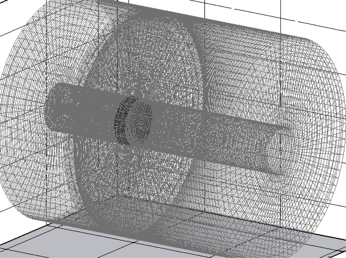
Hybrid grid of computed domain.

The cavitation model mentioned above was introduced to FLUENT code through phase change rate R _e modified by user defined function (UDF) in the computation code. Convection terms in governing equation were discretized with second-order accurate up-wind scheme, while diffusion terms were discretized with the second-order accurate central differencing scheme. SIMPLE segregated algorithm, adapted to unstructured grids, was selected for velocity-pressure coupling. The pointwise Gauss-Seidel iterations were used to solve the discretized equations, and algebraic multigrid method was used to accelerate the solution convergence. The convergence criteria are three orders of magnitude drop in the mass conservation imbalance and four orders in the momentum equation residuals.

The upstream inlet boundary in the computational domain is set as a velocity-inlet where velocity is uniform and equal to the free stream speed U_∞. The inlet boundary was imposed with turbulence intensity at 1% and vapor volume fraction at 0. On the blade surface, regarded as solid wall, zero velocity and no-slip condition were imposed. The downstream exit boundary is set as a pressure-outlet, where pressure is the same as far-field pressure p_∞ and normal derivative of vapor volume fraction is zero. The velocity of the outer boundary (the side of cylinder of computation domain) is the same as that of the inlet boundary. For the periodic boundaries whose intersection angle is 90 degrees, rotational periodicity was ensured. To get faster convergence of the unsteady run and to get more accurate numerical results, the convergence solution of single phase flow was applied as fine initial condition for multiphase computation, and steady solution was applied as fine initial condition for unsteady computation.

There is a relative rotation between the flow fields that are close to the propeller and far away from the propeller in the computational domain. The grids in the two fields are connected through the grid interface along which the grids of the two fields slip relatively. Therefore sliding mesh was adopted to simulate the unsteady flow which varies periodically in the rotating structure. Due to huge calculation amount, parallel computation was adopted so as to reduce computational cost and improve efficiency in the computation.

4. Results

In the following sections, the advance ratio J and the cavitation number σ _n of the propeller are defined, respectively, by J = U_∞/(2nR) and ${\sigma }_n=(p_{\infty }-p_v)/\left(\mathrm{2}{\rho }_l{n}^{\mathrm{2}}{R}^{\mathrm{2}}\right)$ , where n is the propeller revolution speed, the propeller radius R is 0.1135 m, and p_∞ is the reference pressure. The working fluid is water at 20°C, with liquid and vapor densities of 1000 kg/m³ and 0.02558 kg/m³ and saturation pressure of 2368 Pa and surface tension coefficient γ = 0.0717 N/m. The thrust and torque coefficients are, respectively, K _t = Thrust/(16ρ _l n²R⁴) and K _q = Torque/(32ρ _l n²R⁵). The values of σ _n are varied by adjusting p_∞. The effect of number of blades and velocity on wake evolution is investigated on different advance ratio (J = 0.62, 0.75, 0.88) and three kinds of propellers with the same geometry but different numbers of blades. Let n be equal to 25 rps and change U_∞ to get the same intensity of tip vortices and different J.

4.1. Grid Independence

The grid independence study under cavitating and noncavitating conditions is carried out as a measure of numerical uncertainties. The three kinds of grid, as described in the grid generation section, are used to compute the grid convergence index (GCI) of K _t and the axial velocity U _x at a fixed position of wake. According to literature [18], GCI is defined as GCI = 1.25e _a /(λ^θ − 1), where the relative error of solution between coarser and finer grids $e_a^{}=\left|\left({\varphi }_{\text{coarser}}-{\varphi }_{\text{finer}}\right)/{\varphi }_{\text{coarser}}\right|$ . The effective refinement ratio λ is $\sqrt[\mathrm{3}]{\mathrm{2.2}}$ where 2.2 is ratio of grid cells number for different grids. For constant λ, the apparent order θ is calculated using expression $\theta =\left|\ln \left|e_{\mathrm{32}}/e_{\mathrm{21}}\right|\right|/\ln \lambda$ , where e₃₂ = ϕ₃ − ϕ₂, e₂₁ = ϕ₂ − ϕ₁, and ϕ _k denotes the solution of the kth grid. In the noncavitation condition, at J = 0.71 and in the open water, the corresponding value of GCI and e _a for K _t and U _x are presented in Table 1. For cavitating condition, at J = 0.71 and p_∞ = 26821 pa, the values of e _a ²¹ and e _a ³² for K _t are 0.0053 and 0.1061, respectively, and the value of GCI²¹ and GCI³² is 0.004%, 0.7%. The values of e _a ²¹ and e _a ³² for U _x are 0.0175 and 0.00145, respectively, and those of GCI²¹ and GCI³² are 0.2% and 0.017%. Grid has more impact on the results under cavitating condition than those under noncavitating condition. The steady solution of the fine grid is not convergent until iteration reached 2000 steps, while it takes 50 time-steps to be convergent for the unsteady solution. The time step in the paper is set up to 0.25 ms, and the grid rotates 2.25 degrees per time step. The residual of vapor volume fraction is within 0.0008. The other residuals for the fine grid are also within the convergence criteria, so in the paper the fine grid is selected for further calculation.

Table 1:

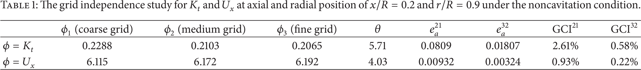
The grid independence study for K _t and U _x at axial and radial position of x/R = 0.2 and r/R = 0.9 under the noncavitation condition.

	ϕ1 (coarse grid)	ϕ2 (medium grid)	ϕ3 (fine grid)	θ	e a 21	e a 32	GCI21	GCI32
ϕ = K t	0.2288	0.2103	0.2065	5.71	0.0809	0.01807	2.61%	0.58%
ϕ = U x	6.115	6.172	6.192	4.03	0.00932	0.00324	0.93%	0.22%

4.2. Numerical Predictions and Validations of Cavitation Extension

The numerical results and validation of the hydrodynamic performance of the propeller E779A under cavitating conditions were presented in [19]. The sheet cavitation evolution in suction side of the propeller blade at different J and σ _n , as shown in Figure 3, demonstrates the effect of velocity and pressure on the cavitation. Here, Reynolds number is 1.29 × 10⁶. The numerical results in Figure 3 show the vapor volume fraction on the back side of blade. Red regions mean vapor, expressing strong cavitation. The results are predicted by unsteady computation and the predictions of the position and extension of the sheet cavitation become stable, when the computation is convergent. Photographs in Figure 3 [20] are captured from cavitation tunnel through sealed window using high-velocity camera, which shows clearly the sheet and tip vortex cavitation. Comparison of experimental and computed results of leading ledge and sheet cavitation illustrates agreement. The cavitation appears at first in the leading edge and tip regions and then develops to form the sheet cavitation at mid-chord with the decreasing of σ _n and J. The numerical vapor volume fraction also indicates that the value is a little high in the center of the blade, which means low pressure. But it is difficult to observe the results in the measured photograph. As illustrated in Figure 3, the cavitation inception is numerically predicted accurately, which is significant to the prediction of cavitation noise for the reason that once cavitation appears, the cavitation noise would become the most important noise resource.

Figure 3:

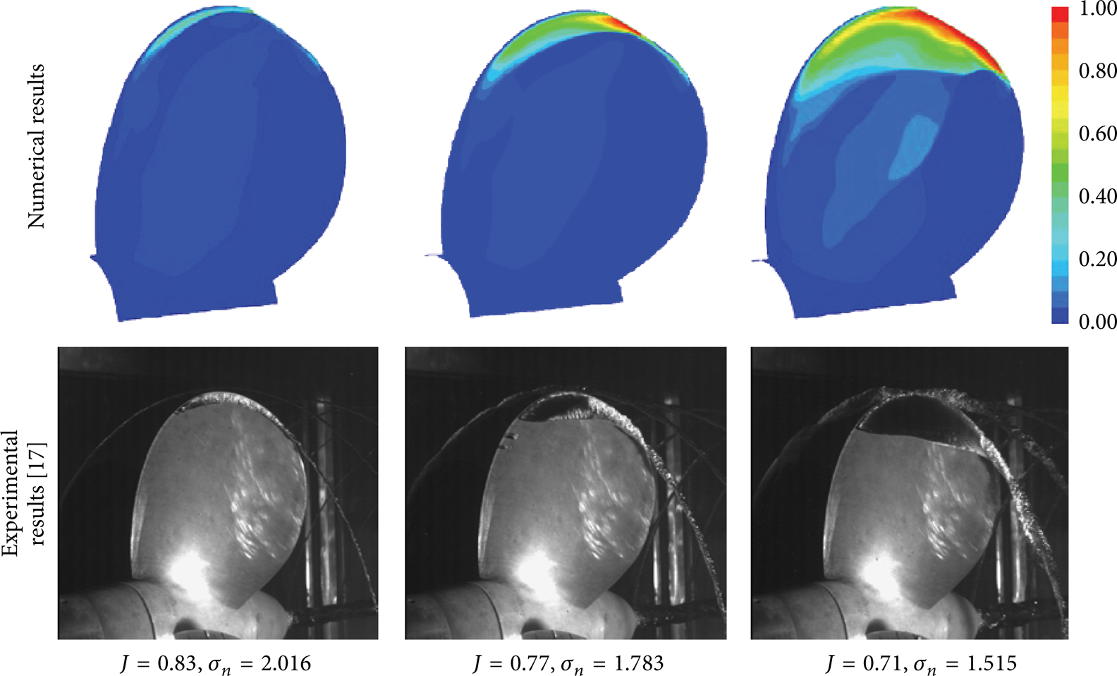
Numerical and experimental results of propeller cavitation.

The numerical results under J = 0.65, σ _n = 1.515, and J = 0.71, σ _n = 1.76 conditions, as shown in Figure 4, illustrate clear cavitation extension, including tip vortex cavitation, which are calculated by refining the grids near the tip vortex region. The cavitation extension shown in Figure 4 is depicted by the black isosurface with vapor volume fraction a _v = 0.2. The correctional full cavitation model and the SST k-ω turbulence model with the boundary layer grids seem to be capable of predicting the tip vortex cavitation.

Figure 4:

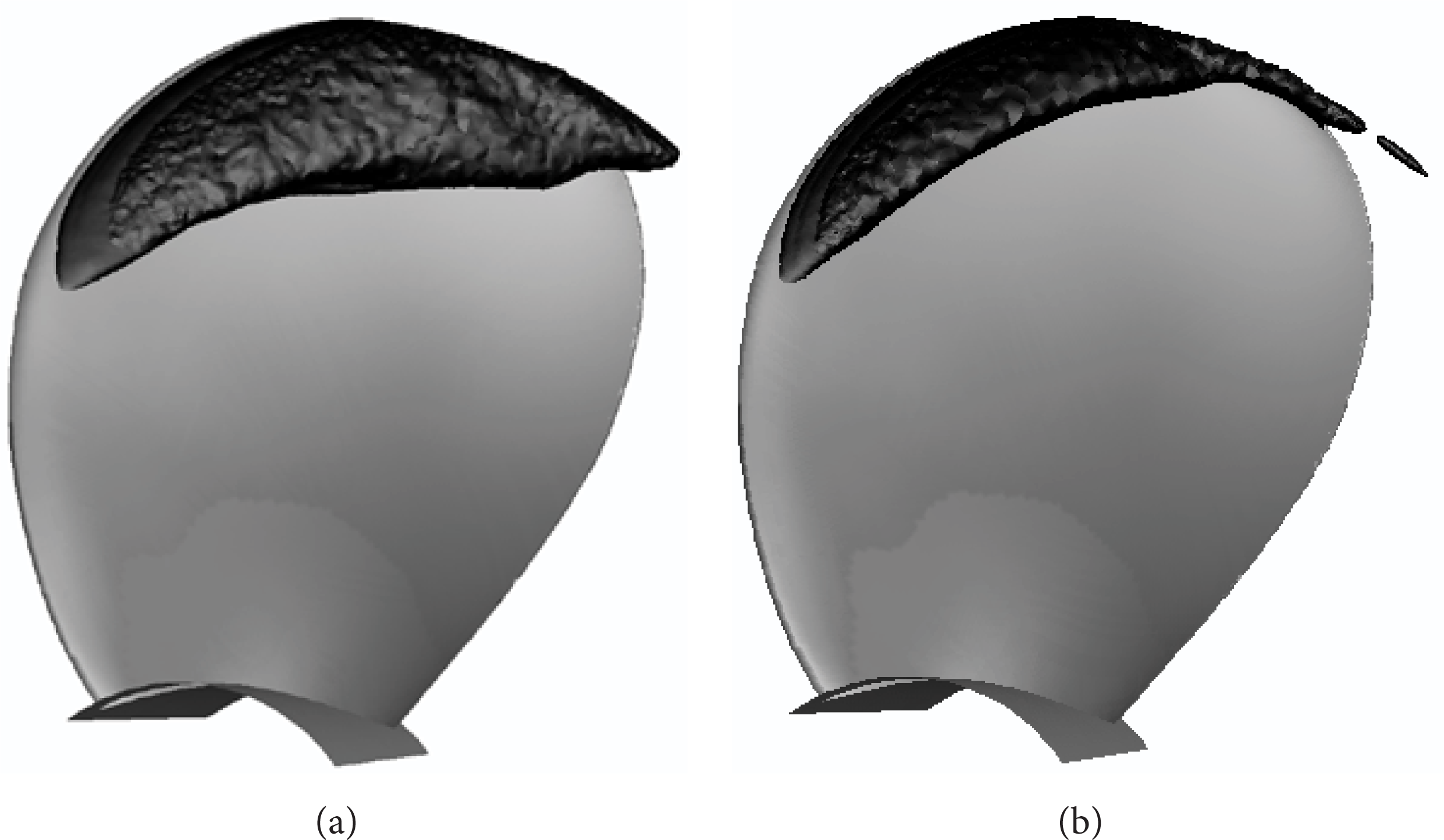
Cavitation predictions (a) J = 0.65, σ _n = 1.515 and (b) J = 0.71, σ _n = 1.76.

4.3. Numerical Predictions and Validations of Normalized Axial Velocity

In this section, the effect of blades on the velocity in transversal planes of onset, interblade, and downstream flow is analyzed through the propellers having different blade number. In Figure 5 the contours display the normalized axial velocity (U _x /U_∞) distribution on the suction and pressure sides of the propeller blades, which reflects the forming and evolution of tip vortex. There are several aspects that may be pointed out. Firstly, the effect of propeller suction on the inflow is apparent as lobes structure in transversal plane of x/R = − 0.6, and the number of blades and the number of lobes coincide with each other. Secondly, from the plane of x/R = − 0.6, the axial velocity starts increasing along inflow direction, reaching its maximum at x/R = 0.0, and then starts decreasing. Thirdly, in the plane at x/R = 0.0 the velocity on the suction side is larger than that on the other side and the maximum value of axial flow acceleration locates at the blade tip where tip vortex occurs. In the plane of x/R = 0.1, the velocity defect curve in correspondence to the blade trailing wake is observed. The tip vortex intensity is weaker than that in the plane of x/R = 0.0 and starts decreasing along inflow direction. At last, for the gradient of axial velocity, the more the blade number, the shorter the interblade distance in transversal plane and the greater the velocity gradient. As shown in Figure 5 in this paper and in Figure 6 in the literature [1], the numerical predictions of maximum value and minimum value of U _x /U_∞ in the transversal planes are 1.62 and 0.5, while the measured data of maximum value and minimum value are 1.45 and 0.5. The numerical distribution shape in the contours of U _x /U_∞ is also close to the experimental results.

Figure 5:

Normalized axial velocity for the two-blade, three-blade, and four-blade propellers: onset, interblade, and downstream flow.

Under J = 0.88 condition, the measured [15, 16] and computed results of normalized axial velocity U _x /U_∞ in three transversal planes for the four-blade propeller are shown, respectively, in Figures 6 and 8. The same numerical results at J = 0.88, x/R = 0.1 are shown in Figure 7 at different unit for easy comparison with measured results. The measured and computed results are well agreement in the transversal plane of x/R = 0.1 and agreement in the far field. For example, in the transversal plane of x/R = 0.1, the maximum value (1.25) of numerical U _x /U_∞ occurs at tip vortex, which coincides with the counterpart measured value (about 1.26). The minimum values of U _x /U_∞ for the numerical and experiment results are 0.75 and about 0.73, respectively. However, there are differences between computation and measurement in the far field where the maximum velocity occurs near tip vortex for experiments and near hub vortex for computation. Mainly because the size of the grid cells in the tip vortex region for the far wake is large, the calculated value of velocity is low. Based on these accurate numerical results, we further numerically investigated the evolution of U _x /U_∞ under J = 0.62 and J = 0.75 conditions. Figure 8 shows U _x /U_∞ distributions of four-blade propeller in the transversal planes at the x/R = 0.1, x/R = 1.0, x/R = 1.5, and x/R = 2.0 downstream axial positions. The distributions illustrate some common features among the three J (J = 0.62, J = 0.75, and J = 0.88). Firstly, the contours of U _x /U_∞ indicate that the axial velocity near the hub is lower and increases outwards along radical direction. Then the axial velocity reaches maximum and starts decreasing to minimum at r/R = 0.9 where tip vortex occurs. Secondly, the axial velocity within propeller wake slipstream tube is much higher than that out of slipstream. It indicates that the propeller thrust only comes from the inner part of the propeller disk, while the outer blade regions are stalled. At last, the apparent axial velocity defect curve in correspondence to the blade trailing wake indicates viscous wake flow which is caused by the blade boundary layer. The positions of the maximum axial velocity and the narrowest defect of viscous flow are both at r/R = 0.4–0.8, which indicates that the thrust of the propeller is mainly generated in the region. Comparing the images in Figure 8, there are several aspects to be pointed out. Firstly, within slipstream tube of propeller wake, the normalized axial velocity and the velocity gradient decrease with the increase of J, which is the same as the propeller thrust. Secondly, near downstream wake, the slipstream shrinks with the increasing distance that is away from the propeller disk. The axial velocity reaches maximum at x/R = 1.0. At last, with the increasing distance away from propeller disk, the velocity gradient and tip vortex intensity at radial position of r/R = 0.9 decrease. At the same time, the curve of the axial velocity defect due to the blade trailing wake becomes longer, its angle becomes larger, blade wake sheets incline more obviously, and at last the interaction between the tip vortex and wake of the next blade occurs. The interaction plays a role in the mechanism of wake instability and the extent of the instability increases with the decrease of J.

Figure 6:

Measured results of normalized axial velocity at J = 0.88 [15].

Figure 7:

Numerical results of normalized axial velocity at J = 0.88, x/R = 0.1.

Figure 8:

Numerical results of normalized axial velocity in wake field at J = 0.62, J = 0.75, and J = 0.88.

The effect of J on the velocity field in propeller wake has been investigated. Now we investigate the effect of the ambient pressure on the propeller wake. The numerical results of axial velocity at two pressures (p_∞ = 26821 pa, 101325 pa) are almost the same, as shown in Figure 9, which indicates weak impact of ambient pressure on the propeller wake.

Figure 9:

Normalized axial velocity at different ambient pressure.

4.4. Evolution of Numerical Axial Velocity and Its Power Spectral Density

The evolution of numerical axial velocity at axial and radial position of x/R = 0.2 and r/R = 0.6 during a period is shown in Figure 10(a). The measured results [16] under the same condition are shown in Figure 10(b). Although the numerical results are a little larger than the measured data, overall the two results are similar. The four waves with similar shape in one period, as shown in the numerical result in Figure 10, reflect four propeller blades action on wake field. The discrepancy among the wave peaks results from grid discrepancy, especially the dissymmetry of the grid of two periodic boundaries. The discrepancy among measured wave peaks results from the dissymmetry of model propeller. In addition, oscillations with very small amplitude due to numerical dispersion make the numerical wave unsmooth, which is different from measured data. But the amplitude of the oscillations is much smaller than that of the whole wave.

Figure 10:

Axial velocity at x/R = 0.2, r/R = 0.6. (a) Numerical results and (b) measured results [16].

The downstream evolution of the power spectral density of the axial velocity at radial position of r/R = 0.3 at three conditions is shown in Figure 11. The evolution shows that at the three conditions the spectrum of the velocity signal is based on the blade frequency at x = 1.5R and then is transformed toshaft frequency (25 Hz) at x = 6R, which reveals some interesting features of propeller wake instability, already pointed out in the literature [1]. However, from comparison among (a), (b), and (c) in Figure 11, the frequency transfer of the two-blade propeller occurs with different mechanism from the four-blade propeller. Specifically, the instability process for the two-blade propeller shows a direct transfer from the blade to the shaft frequency. However, the instability process of the four-blade propeller shows a transfer from blade frequency to 50 Hz at first and then a transfer to shaft frequency. In addition, the transform of the two-blade propeller takes place farther than that of the four-blade propeller. The comparison between (b) and (c) in Figure 11 indicates that the plot at J = 0.71 shows a strong peak of shaft frequency at x = 4R and 6R, while the plot at J = 0.88 shows a visible peak of shaft frequency at x = 4R, and a strong peak of shaft frequency at x = 6R. Therefore, The transform process at J = 0.88 is slower than that at J = 0.71. The amplitude of the signal at J = 0.88 is smaller than that at J = 0.71 which also indicates that load is low at J = 0.88. The above results explain that, at the hub region around r/R = 0.3, the spectrum transforms from blade frequency to shaft frequency with increasing distance from propeller disk. The transfer process becomes quick with increase of J and number of blades. The results of velocity spectrum instability coincide with those of axial velocity in Figure 8. The detail frequency characteristic analysis was included in another paper [21, 22].

Figure 11:

The power spectral density of axial velocity.

5. Conclusions

In the present study, the two important forming mechanisms of cavitation noise, cavitation and wake field behind a ship propeller, are investigated. Comparing computed results with corresponding measured data [1, 2], we draw some conclusions. Firstly, the prediction of E779A hydrodynamic performance coincides with experimental results. The numerical prediction of the forming and development of the sheet cavitation agrees with the experimental results. The tip vortex cavitation extension starts to emerge in the numerical prediction by refining the grids in the region. Secondly, for the three propellers having different numbers of blades, the predictions of axial velocity in transversal planes of onset, interblade, and downstream flows agree with the experimental results. The forming process of tip vortex around propeller blades is illustrated. Thirdly, under J = 0.88 condition, the numerical results of axial velocity at different positions are in agreement with the measured data. The wave shape of axial velocity of a fixing position in a period coincides with the measured results.

Depending on these correct predictions, we investigate further the wake of four-blade propeller at J = 0.62 and J = 0.75. According to numerical results with different J and the far-field pressure, we get other conclusions. Firstly, the normalized axial velocity increases with decreasing J, which reflects the increase of load. Secondly, with increasing distance from propeller disk, the velocity spectrum transforms from blade frequency to shaft frequency. At the same time, the tip vortex of current blade interacts with the wake sheet of the next blade, which makes the wake unstable. The progress of the instability becomes fast with decreasing J. Thirdly, the decrease of the far-field pressure has little impact on velocity field.

Conflict of Interests

The author declares that there is no conflict of interests regarding the publication of this paper.