Sage Journals: Discover world-class research

Abstract

The ride dynamic characteristics of an urban bus were investigated through simulations with suspension component characteristics and were validated through field measurements. It was performed on highway road at a constant forward speed. A random vibration bus model with two parallel tracks of terrain profile was synthesized with superposition between the left and right sides as well as time delay between front and rear. The bus frequency response model was introduced with embedded modal extraction data to enhance computation efficiency. The simulation results of the bus model were derived in terms of acceleration PSD and frequency-weighted root mean square acceleration along the vertical axes at three locations, namely, driver side, middle, and rear passenger side, to obtain the overall bus ride performance. Another two sets of new leaf spring design were proposed as suspension parameter analysis. The simulation approach provides reasonably good results in evaluating passenger perception on ride and shows that the proposed new spring design can significantly improve the ride quality of the driver and passengers.

1. Introduction

Ride dynamics is a critical factor in evaluating the performance of a vehicle. Evaluation of ride dynamics can be carried out either through computer simulation or experimental field data measurements. Experimental results provide accurate data, but tuning the suspension in practical applications is tedious and costly. Nowadays, the ride dynamics of a vehicle has been extensively raised parallel with the significant growth of computation power, which assists in seeking suspension design to provide comfortable ride. A comfortable ride is closely related to the level of vibrations of the vehicle where the passenger is satisfied. Numerous standards for human comfort according to vibration have been published and widely adopted in the automotive industry; examples of these standards include the Janeway comfort criteria (SAE, 1948) and the International Standard ISO 2631-1 [1 –3]. The latter is the most comprehensive ride index and is widely adopted by the researchers worldwide because of its high accuracy.

Originated from a typically simple mechanical-based system, road vehicles have evolved into a complex interdisciplinary mechanical system that includes fluidic and electrical systems. Modern road vehicles are complex mechanical dynamic systems where multiple translational and rotational motions are coupled [4]. The ride dynamics of a vehicle is mostly dependent on the suspension systems installed. Unlike passenger cars, buses utilize different types of suspension systems because of their heavy load carrying capacities. Most buses have leaf springs and large shock absorbers as their secondary suspension system. Generally, leaf springs can be divided into conventional type multileaf springs and parabolic leaf springs. Parabolic leaf springs are widely used in buses as primary suspension system because of their simplicity in structure and less interleaf friction. A conventional multileaf spring has a constant thickness across its length, whereas a parabolic leaf spring has a tapered cantilever profile along its length [5]. Shock absorber is another important element where its damping force versus velocity characteristic affects the ride performance of a bus.

Many researchers have provided insights into vehicle ride comfort design and analysis either through experiments or through simulations. Experimental methods usually utilize time series data for the estimation of the vehicle oscillatory on particular terrain roughness profiles. The time series data are then transformed into frequency domain or power spectral density (PSD) for ride analysis. The simulation method always consists of a numerical vehicle model and predicted road surface excitation as the input to the simulation. The numerical model is built by considering the suspension component characteristics, such as spring stiffness, shock absorber damping force, and tire vertical stiffness. The road input is adopted either from the on-road vehicle data collection or from the virtual proving ground, which is built in simulation software. The actual road profile measurements are complex and involve many instruments; therefore, prediction of road roughness is widely used. Apart from road surface excitations, many other factors affect the ride quality of a bus. These factors include suspension characteristics, vehicle forward speed, vehicle linkage geometry, bus loaded and unloaded conditions, and engine and transmission vibration. Particularly, the effects of suspension parameters on ride comfort analysis of heavy-duty vehicle are worth discussing.

Recently, Pazooki et al. have modeled an off-road forestry skidder with 3D tire-terrain interaction and torsioelastic suspension. The model was validated through field-measured data from an actual vehicle [6]. It is significant to obtain the field-measured data for model validation purpose which most of the published research works have neglected. With the experimental result correlated model, the sensitivities of suspension parameters were determined to establish designs of primary and secondary suspension systems [7]. In the field measurement and correlation analysis performed in [6], a road roughness model of plowed field and pasture was established with the military. A new roughness model was also proposed. For the ride simulation, a torsioelastic forestry skidder model with complex tire-terrain interaction was built. The model was found to have high accuracy. However, the methodology for the 14-degree-of-freedom model built was complicated and time consuming. As for spring design engineers, simplified vehicle model with acceptable accuracy to predict the vehicle model is sufficient. A simple guideline for leaf spring design on vehicle ride analysis is enough for ride estimation. It is significant to have a method to establish the vehicle model in a short period of time for ride analysis purpose.

Another research work by Yang et al. also analyzed the ride comfort in a tractor with tandem suspension by conducting simulations using a multibody dynamic approach with specified road surface roughness [8]. The annoyance rate model was introduced and then validated through simulations and experiments. The ride comfort of the tractor was optimized based on the annoyance rate model. The tedious subjective survey questionnaire conducted in this research actually is devoted to the significant improvement of ride comfort of the vehicle. However, the validation of the suspension component models was not performed. The leaf spring model could be deviated from the actual vehicle tested. Uys et al. conducted an optimization simulation on Land Rover Defender's suspension system with different roads and speeds as parameters through simulation model [9]. This research considered the effects of different speeds and road conditions on suspension tuning. In their model, vehicle interaction between left and right track as well as front and rear was neglected. The neglected part would lead to reduction of result accuracy.

Kumar and Rastogi analyzed the ride dynamics of an Indian railroad vehicle using the vertical acceleration response under different speeds [10]. The railway vehicle was modeled using the bond graph method. The Sperling ride index was implemented to objectively determine the ride comfort of a rail vehicle, whereas Gangadharan et al. constructed a finite element (FE) model of railway vehicle and performed suspension parameter analysis [11]. They used the ISO 2631-1 ride index instead of the Sperling ride index in the analysis. ISO 2631-1 ride standard has been widely adopted by various ground vehicle applications due to its accuracy and complete coverage of frequency range. Yonglin and Jiafan analysed the suspension stiffness and damping on the vibrational behavior of a bus through a Matlab model [12]. In the analysis, the proposed road PSD of asphalt-concrete pavement was used as input to vehicle quarter model, and the ISO 2631-1 ride comfort criterion was implemented to identify the ride quality based on the spring stiffness and shock absorber damping effects. Quarter vehicle model used in the analysis is not sufficient to predict the whole vehicle oscillation behavior and ride quality especially for bus. Bus is a long cantilever vehicle where the response of the vehicle is varying from the front to the end.

The road irregularity, as a stationary ergodic process, is generally illustrated by PSD function in frequency domain. The terrain roughness model in frequency domain provides basic information regarding the ride dynamics of a vehicle. Pazooki et al. compared the acceleration in PSD form from both experimental and simulation methods of a forestry skidder to validate the vehicle model [7]. The acceleration PSD response spectra obtained along the vertical, fore-aft, lateral, pitch, and roll axes of the vehicle were compared and then weighted according to the ISO 2631-1 ride index. Vehicle body acceleration time history data containing the vehicle oscillatory and resonant frequency could be extracted from the data. Meanwhile, the road profile acceleration time domain model contains detailed information on the road. Such detailed information can be regenerated through various methods, such as white noise filtration by Yonglin and Jiafan [12] and artificial neural networks by Ngwangwa et al. [13]. The stochastic time domain model was used to simulate responses on a vehicle for ride comfort analysis [11] and to estimate vehicle response and road friendliness [13, 14]. The natural frequencies of a vehicle on the road can also be estimated by observing the peak of the data after conversion into frequency domain. For actual road excitation PSD measurement, advance instruments and techniques were required. Therefore, ISO has proposed a standard road roughness and wave number for general usage and is widely adopted in automotive industry [15].

In this study, a comprehensive full bus ride dynamic model was derived with integration of shock absorbers, leaf springs, and antiroll bar characteristics to evaluate the suspension design concepts. The bus ride model was formulated through the FE method and solved through a new approach, modal frequency response analysis with superposition between the left and right sides as well as time delay between the front and rear. Road surface excitation input was generated in PSD form through the proposed terrain roughness and wave number for good highway ride as suggested by Wong [16]. The ride dynamic responses of the model were evaluated under excitations representing an equivalent terrain through random response analysis with modal parameters. Ahead of modal frequency response function (FRF) simulations, normal mode analysis was performed to obtain the natural frequencies and mode shapes of the vehicle model. Modal analysis was also conducted to comprehensively determine the vehicle oscillatory behavior. This FRF analysis utilizes modal simplified bus model where other methods do not apply. Previous research simplified the vehicle model, such as half car model [17], and neglected suspension wheel hop [6]. One of the major approaches in this paper is how the modal analysis assists in the bus ride comfort. An experimental field test was performed and correlated with the simulation to validate the modal simulation result.

The bus ride model was used to evaluate the ride performance of a vehicle with suspension characteristics as design parameters. The main objective of this research is to determine the effects of suspension system on bus ride characteristics and to improve suspension module design. In practical applications, the testing method to refine the vehicle ride performance is tedious and costly because real bus and numerous suspension prototype samples are required. Moreover, test equipment and an experienced driver are also required for bus ride testing. Therefore, the simulation method reduces the prototype cost and the development duration of the suspension components. In this study, the simulation procedure was performed to evaluate the suspension systems and to enhance the ride comfort of the bus. The effects of long distance travel in bus on bus driver and passengers with improved suspension design are greater than traditional design because of the less vibration exerted. Prolonged excessive vibration exposure causes sickness feeling, which could cause severe health problems or accidents.

2. Modeling of Suspension Components

Bus is a passenger vehicle that utilizes solid axle as the primary suspension system. A solid axle consists of a central differential in a single housing that also contains the drive shafts that connect the differential to the wheels. The axle is typically suspended with leaf springs and shock absorbers. The axle is also attached to antiroll bars to reduce the body roll of a vehicle during fast cornering or over road irregularities.

2.1. Leaf Springs

The P-2 type parabolic leaf springs used in this analysis are shown in Figure 1 [18]. As shown in the figure, the parabolic leaf spring has parabolic profile from the center to the end of the spring with a gradually reducing thickness. The varying thickness in between is devoted to the stiffness of the spring designed. In most cases, the design of parabolic leaf springs depends on the desired vertical rate, which is relevant to the mass of the vehicle. The vertical rate k for parabolic leaf springs was calculated based on beam deflection theory as follows [18]:

k = \frac{E w_{o} {t_{o}}^{3}}{4 l^{3}} \times C_{V},

(1)

where E is the spring material elastic modulus, t_o is the thickness at the center of the spring, w_o is the width at the center of the spring, l is the length of the cantilever, and C_v is the vertical rate factor. The lateral rate of the parabolic leaf spring was also considered in the design. The lateral rate k_L was calculated as follows [18]:

k_{L} = \frac{E w_{o} {t_{o}}^{3}}{4 l^{3}} \times C_{L},

(2)

where C_L is the lateral rate factor. Subsequently, the stress level of the spring, which extends for the length of spring with parabolic contour thickness, was validated within design limitations. The peak stress, S_o, was calculated as follows [18]:

S_{o} = \frac{6 \times l \times P}{w_{o} {t_{o}}^{2}},

(3)

where P is the vertical load [18]. The vertical stiffness of the parabolic leaf spring adopted in the bus was tested (Figure 2) to compare calculation and experimental value. The eye of the parabolic leaf spring is free to rotate while a vertical load is applied from the centre of the spring. The displacement of the parabolic leaf spring was then measured. The vertical stiffness was calculated based on the force and displacement relationship.

Figure 1:

Leaf spring profile design for (a) front and (b) rear.

Figure 2:

Experimental vertical stiffness test for leaf springs.

2.2. Shock Absorbers

The shock absorber, also known as damper, dissipates kinetic energy. The shock absorber is an important part of an automotive vehicle because it affects ride comfort. The selection of suitable shock absorbers is significant and is divided into three steps. First, the decision of the critical damping of the vehicle sprung mass and unsprung mass is required. The critical damping for the sprung mass and unsprung mass was also considered. The sprung mass critical damping C_cr(s) was calculated as follows [19]:

C_{cr} (s) = 2 \sqrt{K_{R} \times (\frac{W_{s}}{g})},

(4)

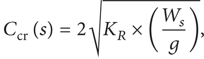
where C_cr is the sprung mass critical damping coefficient, K_R is vehicle ride rate, W_s is the sprung weight, and g is the acceleration due to gravity. The unsprung mass critical damping C_cr(us) was calculated as follows [19]:

C_{cr} (us) = 2 \sqrt{(K_{R} + K_{T}) \times (\frac{W_{s}}{g})},

(5)

where the K_T is tire rate. The damping ratio ε, which is relating the damping coefficient to critical damping coefficient, was calculated as follows:

ε = \frac{C}{C_{cr}},

(6)

where C is the damping coefficient and C_cr is the critical damping coefficient [19]. The damping constant could be obtained from experimental testing as shown in Figure 3. The compression and rebound ratio were then determined. The determination of these parameters is very subjective. The compression and rebound damping speed were obtained based on the decided compression or rebound ratio. Then, damping force and velocity relationship of the absorber was tested experimentally using a damping force tester (Figure 3). The shock absorber was mounted on the damping force tester via revolute joint at the top and bottom. The velocity was set and the damping force was generated during the recording of the piston speed in the shock absorber.

Figure 3:

Experimental shock absorber damping test.

2.3. Antiroll Bars

The front and rear axles of conventional buses had antiroll bars to enhance the roll stiffness of the vehicle. The antiroll bar can be idealized as a torsional stiffener connected between the sprung and the unsprung mass. When the roll bar undergoes a relative rotation between the two masses, the restoring moment M_Φ related to its roll stiffness k_Φ is generated. M_Φ and k_Φ were calculated using (7) and (8) [20]:

M_{Φ} = k_{Φ} (Φ_{s} - Φ_{u}),

(7)

where Φ_s is the roll displacement of the sprung mass and Φ_u is the roll displacement of the unsprung mass [20]:

k_{Φ} = \frac{π G d^{4} l_{b}}{32 {r_{b}}^{2}},

(8)

where G is the shear modulus of antiroll bar material, d is its diameter, r_b is length of trailing lever, and l_b is the effective length of the antiroll bar [20].

3. Full Ride Dynamic Model

Figure 4 shows the process flow of ride improvement analysis of the bus model. Initial stage of the process is to obtain the full bus vehicle model with parabolic leaf spring suspension system. The model of parabolic leaf springs was generated through NX 8.0 CAD commercial software (NX 8.0 is a product of NX under Siemens PLM). The parabolic leaf springs were then preprocessed in finite element software HyperMesh (HyperMesh is a copyright of Altair HyperWorks, Altair Engineering Inc.). Rear and front parabolic springs were assembled to form the suspension module. The shock absorbers were modeled as 1D element and attached in tilted orientation to save space. The parabolic springs were mounted on the solid axle, whereas antiroll bars were attached to the shock eye of the parabolic springs.

Figure 4:

Process flow of ride analysis.

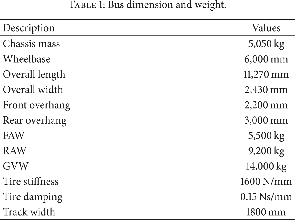
Subsequently, a 10-degree-of-freedom (DOF) ride dynamic model of a bus with 28819 nodes and 33102 elements was developed with six DOFs of bus body and single DOF for each wheel. A schematic diagram of the bus model which complied with ISO 8855 vehicle coordinate system [21] is shown in Figure 5(a). A subassembly of the front suspension module was produced and is shown in Figure 5(b). A similar procedure was carried out for the rear suspension module (Figure 5(c)). The combination of 1D element, 2D quadrilaterals with four nodes in order, and 3D hexahedra with eight nodes was implemented in this case. The 1D element Bar2 was used to model axial, bending, and torsion behaviors. In the FE analysis, the correlation of the stiffness between the FE method and the experimental testing is important. The linear static scheme was applied as preliminary analysis. A few assumptions were made in acceptable engineering standpoint within the simulation. In this model, bus chassis is represented by rigid bodies in ride analysis [22]. Bushings among the joints were also neglected in the simulation. The bus body model with suspension was generated, with the data shown in Table 1. The suspension module is connected to the bus model body through rigid elements. The center of gravity of the bus model was approximated by the front axle weight and the rear axle weight by using force equilibrium assumptions.

Table 1:

Bus dimension and weight.

Description	Values

Chassis mass	5,050 kg
Wheelbase	6,000 mm
Overall length	11,270 mm
Overall width	2,430 mm
Front overhang	2,200 mm
Rear overhang	3,000 mm
FAW	5,500 kg
RAW	9,200 kg
GVW	14,000 kg
Tire stiffness	1600 N/mm
Tire damping	0.15 Ns/mm
Track width	1800 mm

Figure 5:

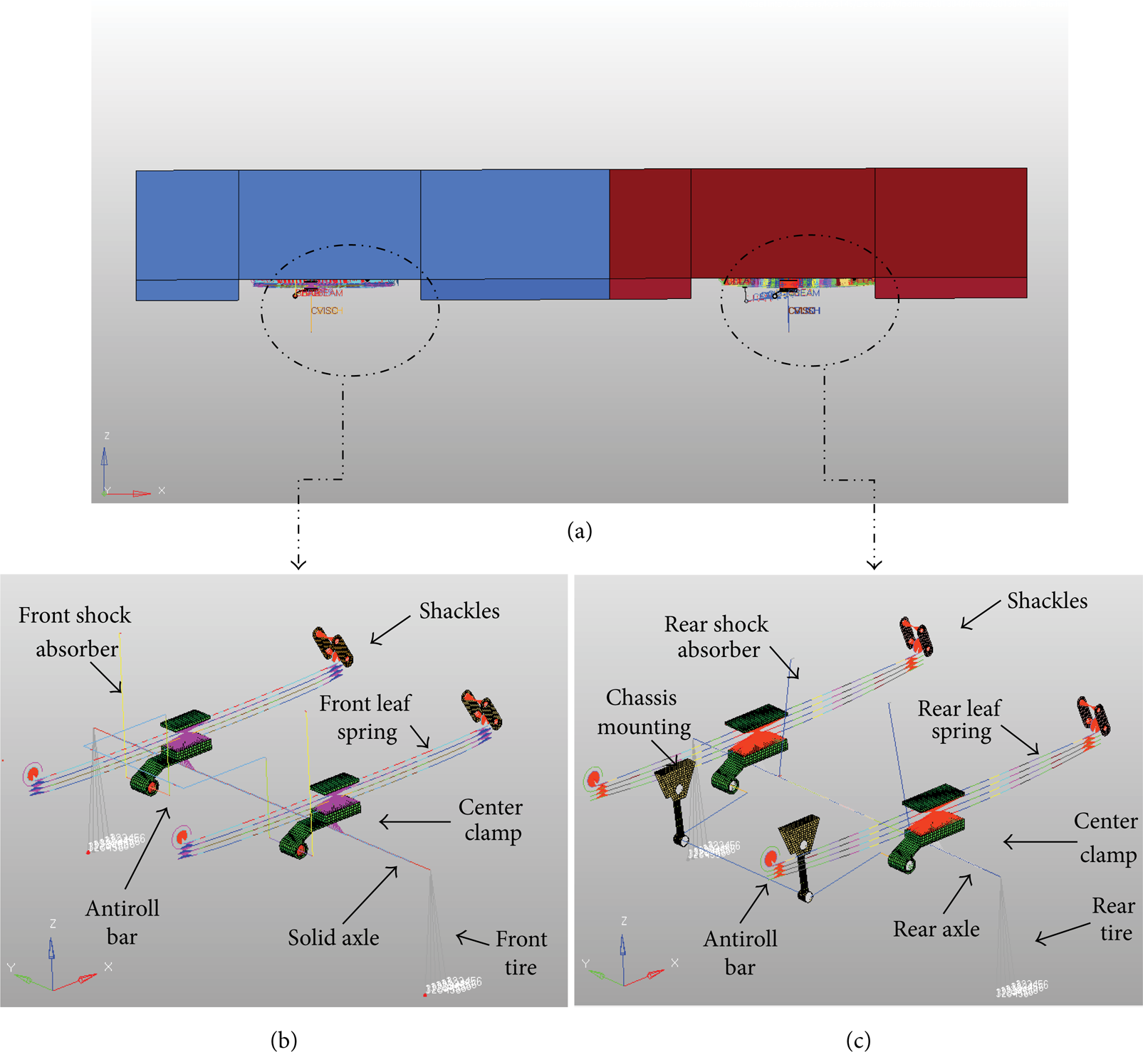
The schematic diagram of (a) 3D bus model body with mass distribution, (b) front suspension module, and (c) rear suspension module.

Modal analysis for frequency response was conducted at the early stage. Vibration analysis was solved either through the Lanczos method or through the automated multilevel substructuring eigenvalue solution (AMSES) method to extract the eigenvalues to be used for modal analysis. In this case, the Lanczos method was adopted towards exact solution. The AMSES provides quick solution but solves only a portion of the eigenvectors. The Lanczos method first reduces the general matrix into the tridiagonal form T_j and finds the solution for the tridiagonal matrix. The general matrix A is the n × n real symmetric matrix. Let v₁ be a unit starting vector, typical generated randomly. Using Lanczos variant recursion, the matrix A was transformed into real symmetric tridiagonal matrices, T_j. The method for extracting the eigenvalues of the tridiagonal form is a variant of the basic QL procedure. The eigenvectors were then calculated through the iterative algorithm. If the displacement w(x, y, z) is written in terms of eigenvectors Φ_i(x, y) and the time dependent modal coordinate q_i(t) as [23]

w (x, y, t) = \sum_{i = 1}^{n} Φ_{1} (x, y) q_{i} (t),

(9)

then the eigenvalues and the corresponding eigenvectors calculated from the tridiagonal matrix are [23]

[K] {Φ_{i}} = {ω_{i}}^{2} [M] {Φ_{i}} .

(10)

Based on the orthogonal properties of the eigenvectors, the expressions for resonant frequencies and corresponding mode shapes were given by [23]

{Φ_{i}}^{T} [K] {Φ_{i}} = {ω_{i}}^{2} {Φ_{i}}^{T} [M] {Φ_{i}} .

(11)

Let {Φ_i}^T[K]{Φ_i} = K_i and {Φ_i}^T[M]{Φ_i} = M_i. Then we get

{ϖ_{i}}^{2} = \frac{K_{i}}{M_{i}},

(12)

where K_i and M_i are, respectively, the stiffness and mass of the structure in ith mode corresponding to the eigenvector Φ_i and the resonant frequency ω_i [23]. The measured frequency range, which is the output request for a frequency within 0.1 Hz to 80 Hz, was requested. The vehicle ride vibration due to excitation contributions from road surface roughness ranged from 0.3 to 28 Hz [24], as proposed by Kawamura and Kaku, and the frequency of interest ranged from 0.5 Hz to 50 Hz, as recommended by Kawamura and Kaku [25]. Therefore, the output frequency up to 80 Hz is sufficient to cover the analysis due to road disturbances.

4. Excitation from Road Surface

The PSD of the roughness of smooth highway road in good condition, as a function of temporal excitation frequency, was expressed as follows [16]:

Φ_{ξ} (f) = \frac{c_{s p} \times V^{N - 1}}{f^{N}},

(13)

where f is the temporal excitation frequency of excitation, V is the velocity of the bus, C_sp is the road roughness coefficient, and N is the wave number. The values of the road roughness coefficient C_sp and the wave number N for the asphalt smooth highway in good condition proposed by the ISO are listed in Table 2.

Table 2:

ISO roughness coefficient and wave number for the smooth highway.

Pavement type and condition	N	C _sp

Smooth highway	2.1	4.8 × 10⁻⁷

Apart from the wave number and road roughness coefficient, the bus speed was determined to be 20 m/s (72 kph). The frequency range of 0.1 Hz to 50 Hz was adopted because the road roughness on a particular frequency range had the most significant impact on the vehicle oscillatory behavior. The present study of the PSD with the parameters considered was plotted and compared with ISO road classification (Figure 6). As shown in Figure 6, the present study on smooth highway road was categorized as Class B (good road condition). The PSD of the smooth highway road was used as road excitation input to the simulations.

Figure 6:

Road roughness classification by ISO (20 m/s).

5. Random Vibration

Excitation from the ground was described as random function to provide more realistic results of bus ride characteristics. The instantaneous value of a random function cannot be predicted in a deterministic manner. The road profile encountered by the wheels of a vehicle is made up of a series of bumps and depressions that cannot be predicted. However, the road profile could be defined as a stationary ergodic process where the ensemble measurements have statistical features that are independent of time and where temporal average is the same for all ensemble measurements. The mean and standard deviation of the recorded acceleration time history will not change over time. PSD specification, which defines load set PSD factors, was used in the random analysis.

If H_xa(f) and H_xb(f) are the complex frequency responses due to the load cases a and b, respectively, then the PSD of the response is as follows [25]:

R_{x} (f) = H_{x a} (f) S_{a b} H_{x b} (f),

(14)

where S_ab(f) is the PSD of the two sources, the individual source a is the excited load case, and b is the applied load case. The cross spectral density S_ab(f) with two different sources could possibly be a complex number. The autocorrelation function A_x(τ) for an ergodic stationary process of variable y can be defined as [25]

A_{x} (τ) = \lim_{t \to \infty} \frac{1}{T} \int_{- (T / 2)}^{T / 2} y (t) y (t + τ) d t .

(15)

The root mean square value of the response y(t) can be written as follows:

y_{rms} = \sqrt{\int_{- \infty}^{\infty} S_{x} (f) d f},

(16)

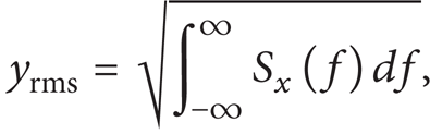
where S_x(f) is a function of PSD [25].

The complex frequency response can be achieved by modal frequency response. The PSD function of the input is defined as a tabular function of frequency for use in random analysis. The PSD function of the input was obtained through on-road data experimental method. The modal frequency response function was set up for this random vibration analysis. The input is the combination of dynamic loads and transformed into modal coordinates using the eigenvectors [23]:

[- Ω^{2} X^{T} M X + X^{T} K X] d e^{i Ω t} = X^{T} P e^{i Ω t} .

(17)

The modal mass matrix X^TMX and the modal stiffness matrix X^TKX are diagonal. If the eigenvectors are normalized with respect to the mass matrix, the modal mass matrix is the unity matrix and the modal stiffness matrix is a diagonal matrix holding the eigenvalues of the system. This way, the system equation is reduced to a set of uncoupled equations for the components of modal response d that can be solved easily. The nodal transformation method has been applied for dynamic transformation-tapered Timoshenko beam in [26].

The collected vibration signal from the road that was converted into PSD function was used as the input into the random vibration function. To use the modal frequency response, dynamic load tabular function, which is a frequency-dependent dynamic load for frequency response problem, is defined as [27]

f (Ω) = A * B (Ω) e^{i (φ (Ω) + θ - 2 π Ω τ)},

(18)

where A is applied load and B is coefficient for generating frequency-dependent dynamic loads. For the rear side, a function of time lag is assigned. The time delay τ is defined as [26]

τ = \frac{(a + b)}{V},

(19)

where a and b are the distances from the center of suspension to the center of mass of the vehicle from the front and rear, respectively, and V is the vehicle speed [26]. In this study, the front and rear dynamic load superposition function was applied to combine the load sets of the front and rear. The left and right sides of the front and rear responses of the function were combined into the front and rear functions.

After a complete list of the dynamic load tabular functions, a set of frequencies for the modal method of frequency response is analyzed by specifying the number of frequencies between modal frequencies. In order to obtain a better resolution near the modal frequencies where the response variation is highest, a cluster value is applied according to the equation [27]

f_{k} = \frac{1}{2} (f_{1} + f_{2}) + \frac{1}{2} (f_{1} + f_{2}) {| ζ |}^{1 / cluster} * SIGN (ζ),

(20)

where ζ = − 1 + 2(k − 1)/(NEF − 1), a parametric coordinate between −1 and 1:

k = excitation frequency in the subrange;

f₁ = frequency at the lower limit of the subrange;

f₂ = frequency at the upper limit of the subrange;

NEF = the number of excitation frequencies.

The insertion of a cluster value provides either a closer spacing of excitation frequency towards the ends of the frequency range or a closer spacing towards the center of the frequency range, depending on the cluster index [27]. In design optimization, the excitation frequencies are derived from the modal frequencies computed in each of the design iterations.

6. Results and Discussions

A basic characteristic of parabolic leaf springs is force-displacement dependence. The vertical stiffness of the parabolic spring is defined as the load per unit deflection of the spring. The vertical stiffness of the parabolic leaf spring can be obtained through an experimental setup as shown in Figure 2. The results of the experimental tests are plotted in Figure 7. As seen in Figure 7, the vertical stiffness of the front and rear parabolic leaf springs remains constant before they fall in the plastic region. The front parabolic leaf springs have a vertical stiffness of 278 N/mm, whereas the rear parabolic leaf springs have a vertical stiffness of 406 N/mm. For the bus model, the vertical stiffness of the rear parabolic leaf spring is higher than that of the front, as a result of the difference in the weight distribution of the bus. The engine of the bus is located at the rear side, and thus the rear parabolic leaf springs acquire a higher load carrying capacity. For the damping of the bus, the shock absorber is characterized by nonlinear force-velocity dependence. The damping force and piston speed relationship is obtained through an experimental setup as shown in Figure 2. Figure 8 depicts the nonlinear characteristic of the shock absorber in terms of the damping force and piston velocity. The damping force versus velocity plot shows a nonlinear piecewise relationship. Different speeds exerted on the piston produce different rebound forces. In general, speeds are classified as low, medium, and high range.

Figure 7:

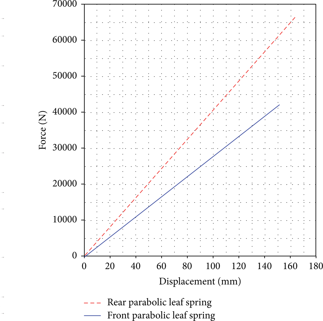
Parabolic leaf spring load versus displacement curve.

Figure 8:

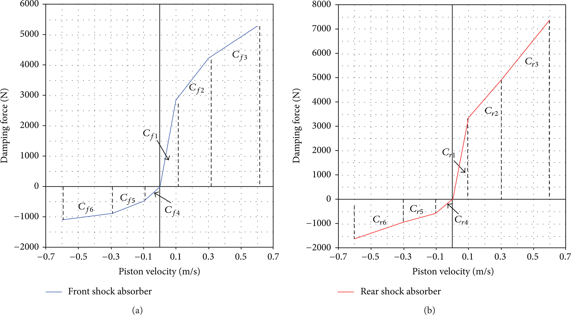
Shock absorber damping force versus velocity curve: (a) front and (b) rear.

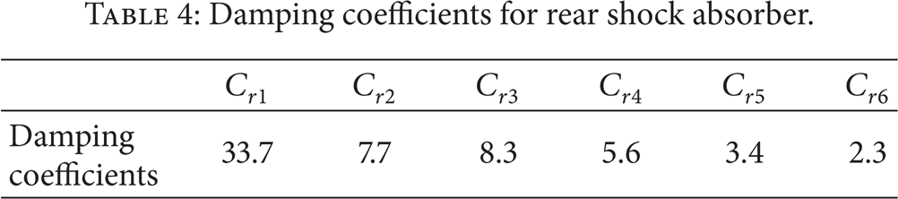
The driving speed of the bus has a direct impact on the shock absorber piston velocity. As seen in Figure 8, the rebound damping force is higher than compression because of the shock absorber inner valve and control disc settings. A higher piston speed leads to a greater rebound force generation. The damping coefficients for the front and rear shock absorber are shown in Tables 3 and 4, respectively. The linear data of the front and rear shock absorber are summarized in Tables 5 and 6, respectively. The damping coefficients are represented by the gradient of the piecewise linear curve. The rebound and compression damping reduction factors for the front shock absorber are calculated as 0.12 and 0.16, respectively, whereas the rebound and compression damping reduction factors for the rear shock absorber are 0.25 and 0.41, respectively. The damping coefficients are the primary inputs for the shock absorber. For the simulations, the vehicle speed is about 20 m/s. The damping coefficients of the medium range were chosen for the preliminary study. The compression forces of the shock absorbers exert less influence on the vehicle ride dynamics.

Table 3:

Damping coefficients for front shock absorber.

	C _f1	C _f2	C _f3	C _f4	C _f5	C _f6

Damping coefficients	28.4	7.0	3.5	4.5	2.2	0.7

Table 4:

Damping coefficients for rear shock absorber.

	C _r1	C _r2	C _r3	C _r4	C _r5	C _r6

Damping coefficients	33.7	7.7	8.3	5.6	3.4	2.3

Table 5:

Front shock absorber damping force and piston speed.

Piston speed (m/s)	Rebound force (N)	Compression force (N)

0.1	2840	450
0.3	4240	880
0.6	5280	1090

Table 6:

Rear shock absorber damping force and piston speed.

Piston speed (m/s)	Rebound force (N)	Compression force (N)

0.1	3370	560
0.3	4900	900
0.6	7400	1600

A bus is a passenger vehicle that may be considered as a compound structure made up of many mechanical components subject to variable loadings. The ride dynamics of a bus rely on the stiffness of its suspension systems and overall mass. To analyze such dynamics, an FE approach modal analysis was performed to acquire the natural frequencies and mode shapes of the urban bus model. This approach provides the vibration behavior of the bus according to the stiffness of the suspension systems and body mass. Based on the FE modal analysis results, the first mode of baseline model is identified as the roll mode of the bus model as shown in Figure 9(a). The second and third modes of the analysis show the bounce and pitch modes of the bus model as illustrated in Figures 9(b) and 9(c), respectively. The fourth and fifth modes are known as the suspension wheel hop mode, where the deformation of the suspension is the largest at this particular frequency. The axle of the leaf spring moves upward and downward in large displacements and the leaf springs are drastically deformed as shown in Figures 9(d) and 9(e). Road excitations are classified into low frequency excitations. A guideline for this simulation is the mode shapes with natural frequencies that range from 0.3 Hz to 28 Hz, which are associated with road profile excitation [22]. Based on (12), higher system stiffness leads to higher natural frequencies of the system. Based on the results obtained, the bus model bounce mode frequency is exorbitant and appears to be in the second mode. The first roll mode of the bus consists of a natural frequency of 2.37 Hz. The second and third modes, which are the bounce and pitch modes, consist of frequencies 2.85 and 4.99 Hz, respectively. The suspension wheel hop mode is at 9.77 Hz (rear) and 11.44 Hz (front).

Figure 9:

Variation of mode of the bus body model produced from FE analysis-based modal analysis: (a) roll mode, (b) bounce mode, (c) pitch mode, (d) front suspension bounce mode, and (e) rear suspension bounce mode.

An experimental setup that measures the vertical acceleration of the bus was conducted on smooth highway roads. To collect the acceleration signal, an accelerometer was embedded on the middle of the floor of the passenger location. The time history of the acceleration signal is shown in Figure 10. The sample data was collected at a sampling rate of 50 Hz and a sample length of 25 s to ensure that sufficient information was gathered. In order to obtain the natural frequencies of the bus, the fast Fourier transform (FFT) method was utilized to convert the time domain into a frequency domain [28]. Figure 11 depicts the frequency domain of the vertical acceleration. The peak amplitude of acceleration was observed at frequencies of 2.65, 9.35, and 10.60 Hz. Natural frequencies of the simulated vehicle bounce mode were at 2.85 Hz, whereas the rear and front suspension bounce modes were at 9.77 and 11.44 Hz, respectively. For the bus body bounce mode, FE modal simulation results deviated slightly from the experimental testing results because of the rigid chassis, tire properties, neglected bushing, and so forth. However, the differences between the simulation and experiment still fell within a good correlation, and thus the simulation model was valid for further use for ride comfort analysis. The longitudinal roughness of the pavement is of a stochastic nature and has different wavelengths and amplitudes. In order to obtain the accurate vehicle oscillatory behavior, a random vibration setting was embedded into the vehicle modal model. Following the random PSD road excitation proposed in Figure 6, the vertical acceleration time series data of the passenger seat location in the bus body was measured. To derive the overall bus ride performance, multiple points of vehicle response were requested from the FE simulation. Figure 12 depicts the details of the location where the response of the driver and passengers was measured. Three different locations were identified as response measurement points: the driver, passenger A, and passenger B. The driver's location was in the front position of the bus body. Passenger A was assigned in the middle of the bus body. Passenger B was assigned at the rear of the bus. The rms value of the acceleration reflects the intensity of the vibrations, and it was used to evaluate the influence of the vibrations on comfort. For simplicity, the analysis used the driver and the different passenger floor locations for the evaluation of the performance. The response at the driver and the two passenger locations were obtained based on the bus body bounce and pitch motions and the kinematic relation for the location.

Figure 10:

Experimental time history of vertical acceleration (passenger A).

Figure 11:

Frequency domain of vertical acceleration.

Figure 12:

Location of vehicle response measurement.

Figure 13 indicates the measured vertical acceleration of the baseline bus model from the location as shown in Figure 12. Based on Figure 13, the peak acceleration value for the preliminary analysis concentrated on the vehicle bounce and pitch mode frequencies, as well as the suspension wheel hop mode. The peak vertical acceleration on the driver position is highest at the vehicle pitch frequency whenever the passenger position's peak is located at the bounce frequency. The driver region consists of the highest PSD acceleration amplitude of 41.17 (m/s²)²/Hz at pitch frequency 4.99 Hz, whereas the second peak amplitude of PSD acceleration of 13.00 (m/s²)²/Hz is at frequency 30.89 Hz. The bounce frequency has a peak amplitude of 2.71 (m/s²)²/Hz, which is less significant compared with the others. For passenger A region, the peak amplitude of PSD acceleration is around 2.85 Hz to 3.09 Hz, the same range for the region of the bounce frequency. The peak amplitude of PSD acceleration is 10.06 (m/s²)²/Hz at 3.09 Hz, whereas the second peak amplitude of PSD acceleration is 6.64 (m/s²)²/Hz at the rear suspension wheel hop mode's frequency of 9.24 Hz. Passenger B experiences peak PSD acceleration amplitude at a frequency of 3.08 Hz for a magnitude of 19.80 (m/s²)²/Hz. Another peak amplitude of PSD acceleration is observed at frequency 10.14 Hz, where the PSD vertical acceleration is 16.26 (m/s²)²/Hz. A few assumptions were made for the simplicity of the model. Tire properties and ground interaction were neglected. Bushing, linkages, and chassis were represented in rigid form. Each of the simplifications caused the rms acceleration to be higher than the actual bus.

Figure 13:

Power spectra density of (a) driver's vertical acceleration, (b) passenger A's vertical acceleration, and (c) passenger B's vertical acceleration.

After the power spectra density of the point was obtained, further analysis related it to any ride comfort criterion available. In compliance with ISO 2631-1, the frequency-weighted rms acceleration is recommended [3]. The overall frequency-weighted acceleration should be determined by weighing and the appropriate addition of a narrow band or a one-third octave band data over the frequency range of interest. Prior to that, the transformation of power spectra density into rms values of acceleration as a function of frequency is necessary. As proposed, the rms value of acceleration at each center frequency can be calculated as [3]

a_{i} = \sqrt{\int_{0.89 f_{c}}^{1.12 f_{c}} s_{v} (f) d f},

(21)

where a_i is the rms acceleration, f_c is the center frequency, and S_v is the power spectra density function for the acceleration. After obtaining the rms values, the conversion of the one-third octave band data is performed with the ISO weighting factors as indicated in Figure 13. The overall frequency-weighted acceleration is determined through the equation [3]

a_{w} = \sqrt{\sum_{i} {(w_{i} a_{i})}^{2}},

(22)

where a_w is the rms of the weighted vertical acceleration, W_i is the weight factor of the ith central frequency of the one-third octave band excitation range, and a_i is the rms of the acceleration of the ith central frequency of the one-third octave band excitation range [3]. As can be observed from Figure 14, the vertical weighting factor W_k is the highest in the frequency range of 4 Hz to 8 Hz. The principal weighting curve defines human sensitivity towards vertical vibration as the most significant at a particular range of frequencies. The vehicle bounce and pitch modes are the major contributions to the vertical vibration. Passenger comfort on the road depends on the bounce and pitch motion of the vehicle [29]. In order to prevent the discomfort in a vehicle ride, the ride mode (bounce and pitch) of the vehicle must be lower than 4 Hz to prevent excessive vertical vibration. Further, motion sickness, which is derived from the vertical vibration, also needs to be taken into consideration. The vibration of vertical motion sickness is in the range of 0.1 Hz to 1 Hz. Discomfort frequencies range from 4 Hz to 10.5 Hz [30]. The optimum comfort zone for the vehicle body to bounce and pitch motion is hence designed within a range of frequencies greater than 1 Hz and less than 4 Hz.

Figure 14:

ISO 2621-1:1997 frequency weighting curves for principal weightings.

Different vehicle designs and operating parameters, including the linkage between components, vehicle forward speed, vehicle load, and terrain roughness, affect the ride performance of the vehicle. Suspension characteristics also influence the load carrying capacity of the vehicle instead of the vehicle ride. In this analysis, the suspension characteristics of the bus model are used to study the sensitivity of ride responses to variations and to seek desirable suspension designs. The modification in suspension systems influences the bus riding response of the front, middle, and rear passengers, respectively. Different positions in the bus body exhibit different vibration responses, and thus three points in the bus as recommended in Figure 12 are acquired for a holistic bus ride analysis. Frequency-weighted vertical acceleration results for the baseline model are summarized in Table 5. Frequency-weighted rms acceleration indicates the sensation of the passenger base in relation to human sensitivity, whereas the unweighted frequency rms acceleration reveals the overall bus ride performance. Passenger A experiences the highest level of comfort compared to the driver and to passenger B. The region between the front and rear suspensions experiences less vibration because of road excitations and is considered the most comfortable region of a bus. The driver and passenger B regions experience higher amplitude of acceleration when the vehicle oscillates as shown in Table 7. For suspension design purposes, a sensitivity analysis of suspension parameters has been carried out by altering the leaf spring stiffness and shock absorber damping coefficients. The frequency-weighted and unweighted accelerations for three prescribed points are listed for a detailed description of the whole bus ride analysis.

Table 7:

Comparison of frequency-weighted accelerations of driver and passengers.

	Driver	Passenger A	Passenger B

Frequency-weighted accelerations	30.0	10.8	27.8

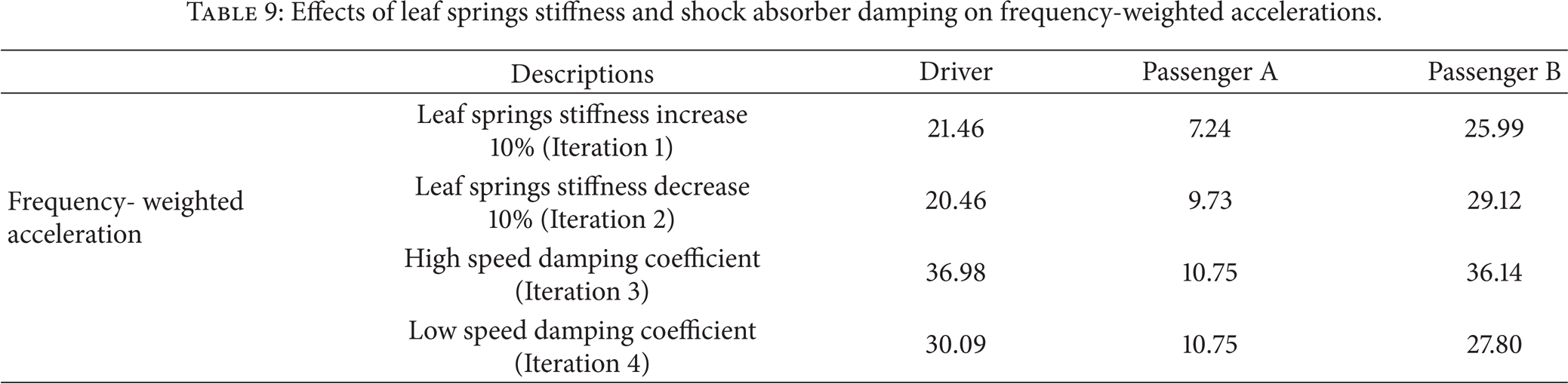
To classify the modification on the suspension parameters, the increase of leaf springs stiffness is called “Iteration 1,” whereas the reduction of leaf spring stiffness is called “Iteration 2”. Iteration 3 is the utilization of high speed damping, whereas Iteration 4 is the utilization of low speed damping. The original bus suspension is tagged as the baseline. A modal analysis is performed against the changes of suspension parameters. Natural frequencies in Iteration 1 are observed. The first mode is at 2.31 Hz, followed by the second at 2.44 Hz and the third at 4.32 Hz. The rear and front suspension wheel hop modes are at 9.70 and 11.44 Hz, respectively. The natural frequencies of Iteration 2 are at 2.30 (roll mode), 2.60, 4.25, 9.82 Hz, and 11.44 Hz as shown in Table 8. Compared with Iteration 1, the frequency of the bus roll mode is reduced when the spring stiffness is reduced. Nevertheless, the second mode, the bus bounce mode, is shifted from a pure bounce mode to a mixed mode combining the roll and bounce modes. The mixed mode is detrimental to the ride dynamics of the bus because a higher acceleration is exerted on the vehicle body. The gap of the frequencies between the first and second modes is too small where the resonance can happen simultaneously. The first mode of Iteration 2 is the roll mode, and the second mode is the mixed mode. The natural frequency of the pitch mode is reduced for both Iterations 1 and 2. When comparing the rear suspension wheel hop mode of Iteration 1 to the baseline model, the natural frequency is shifted from 9.77 Hz to 9.70 Hz. This shift implies that the reduction in the stiffness of a system exhibits a reduction in natural frequency [23]. On the contrary, in Iteration 2, an increase in the parabolic leaf spring vertical stiffness produces an increase in natural frequency from 9.77 Hz to 9.82 Hz. Although the variation in the natural frequency is exorbitant, the influence on ride performance noticeably varies. The front suspension wheel hop mode for both Iterations 1 and 2 does not undergo significant changes in natural frequency when the vertical stiffness of the parabolic leaf spring is altered. By contrast, a slight change occurs in the rear suspension wheel hop mode. The changes in suspension wheel hop mode are affected by the mass distribution of the bus. A small change in leaf spring stiffness produces minor effects in the natural frequency. Shock absorber damping, another suspension element, is also considered in this analysis. Complex eigenvalue analysis is performed when the damping of the mode is included. Real eigenvalue analysis is used to compute the normal modes of a structure, whereas complex eigenvalue analysis is used to compute the complex mode of the structure. In this analysis, damping is computed as an imaginary part, which has no effect on the real eigenvalue. Therefore, the natural frequencies are observed to be the same as the baseline design.

Table 8:

Natural frequencies of vehicle modes obtained through suspension variations.

	First mode, Hz(roll mode)	Second mode, Hz(bounce mode)	Third mode, Hz(pitch mode)	Fourth mode, Hz (rear wheel hop)	Fifth mode, Hz (front wheel hop)

Baseline design	2.37	2.85	4.99	9.77	11.44
Iteration 1	2.31	2.44	4.32	9.70	11.44
Iteration 2	2.30	2.60	4.25	9.82	11.44
Iteration 3	2.37	2.85	4.99	9.77	11.44
Iteration 4	2.37	2.85	4.99	9.77	11.44

Road profile excitation is given in all suspension changes that seek ride enhancement. A comparison of the PSD acceleration of all iterations is plotted in Figure 15. From Figure 15(a), passenger A is the most significant region because most of the passengers are concentrated in this region. Based on Figure 15(b), the PSD acceleration of the human sensitivity region at 4 Hz to 8 Hz is considerably low. Iteration 2 yields a higher peak PSD acceleration at frequency 2.78 Hz with 12.86 (m/s²)²/Hz. The PSD acceleration of Iteration 3 shows a great reduction of peak amplitude at frequency 9.77 Hz. However, the PSD acceleration in the range of 4 Hz to 8 Hz is increased drastically. This increase means that an overwhelming damping force is causing much discomfort to the bus. Low speed damping (Iteration 4) has insignificant differences from the original design. The rear passenger region experiences less comfort when compared to the middle passenger region. Based on the peak and trend analysis from Figure 15(c), an increase in parabolic leaf spring stiffness directly affects the pitch mode and PSD acceleration around the critical region with which the ride comfort of the rear passenger and the driver is associated.

Figure 15:

Comparison of vertical acceleration PSD of bus model on baseline, Iterations 1, 2, 3, and 4 of position (a) driver, (b) passenger A, and (c) passenger B.

The frequency-weighted accelerations of all iterations are summarized in Table 9. An increase in leaf spring stiffness leads to a significant decrease in frequency-weighted acceleration, especially at the driver region. By contrast, a reduction of leaf spring stiffness also leads to a reduction of frequency-weighted accelerations. This decrease indicates that the ride quality of the driver of this bus model is improved either through an increase or through a decrease in leaf spring stiffness. From the perspective of passengers A and B, a reduction in leaf spring stiffness obviously leads to a reduction in frequency-weighted acceleration. Subsequently, the whole bus ride quality is raised with a reduction in leaf spring stiffness. Less stiff springs yield smaller peak amplitude of acceleration on the bus body and allow for a greater ride index. To target the improvement of bus riding, reduction in acceleration is necessary at the middle region, where most of the passenger seats are located. At the same time, the driver's perception must be taken into consideration. In this case, the reduction of leaf spring stiffness successfully fulfills the requirement of reducing the frequency-weighted acceleration and enhances the ride quality of the bus. In another case, the effects of shock absorber damping modifications are considered. When shock absorber high speed damping coefficient is applied in the model, the frequency-weighted acceleration is drastically increased in the region near the driver, passenger A, and passenger B. The damping force generated is overage and causes discomfort to the whole bus. By contrast, the frequency-weighted acceleration of the passenger is increased when a low speed damping coefficient is induced. However, no significant changes occur in the PSD acceleration between the shock absorber damping coefficients for low and medium speed damping. The medium speed damping coefficient indicates the primary input of the original design. The damping force generated during low and medium speeds is suitable to this driving condition.

Table 9:

Effects of leaf springs stiffness and shock absorber damping on frequency-weighted accelerations.

	Descriptions	Driver	Passenger A	Passenger B

Frequency- weighted acceleration	Leaf springs stiffness increase 10% (Iteration 1)	21.46	7.24	25.99
	Leaf springs stiffness decrease 10% (Iteration 2)	20.46	9.73	29.12
	High speed damping coefficient (Iteration 3)	36.98	10.75	36.14
	Low speed damping coefficient (Iteration 4)	30.09	10.75	27.80

Traditionally, the vehicle ride analysis was performed through frequency response analysis. A new approach, modal frequency response function, has been performed to identify the output response of the bus body. Compared to the traditional frequency response analysis, the time for solving the LTI systems has been reduced significantly. The modal FRF model could be solved within few minutes while the conventional FRF model may take few days to complete. This allows the suspension designer to perform modifications on suspension design and to analyse their performance in a short period. Meanwhile, high computational power is required for conventional FRF model where cost of computing power is high. This method extracts the eigenvalue of the linear vehicle system for the analysis. Therefore, the matrix is tridiagonal and solution for the matrix is faster.

7. Conclusions

This study developed a comprehensive full bus ride dynamic FE model by integrating the simplified tire, shock absorbers damping, leaf spring stiffness, and antiroll bar roll resistance characteristics. The vehicle dynamic of a bus was described in mode shapes and natural frequencies through a modal analysis. The modal analysis results showed the natural frequency change with respect to parabolic leaf spring stiffness. The variation of natural frequencies significantly affected the ride quality of the bus due to resonance effect. Based on the results, a new parabolic leaf spring design with 10% stiffness reduction enhances the ride index of the driver, middle, and rear passenger by 28.5%, 33%, and 7%, respectively, compared to the original leaf spring design. The overall ride quality of the bus has improved. Besides, through the implementation of recommended modal FRF analysis, the ride quality of the bus improved with minimum spring and shock absorber prototype samples.

Conflict of Interests

The authors declare that there is no conflict of interests regarding the publication of this paper.

Footnotes

Acknowledgments

The authors would like to acknowledge the financial support from Universiti Kebangsaan, Malaysia (research grant “Industri-2012-037”) and APM Engineering & Research Sdn Bhd.

References

Janeway

R. N.

, Vehicle Vibration Limits to Fit the Passenger, Society of Automotive Engineers, New York, NY, USA, 1948.

Janeway

R. N.

, “Passenger vibration limits,” SAE Journal, vol. 48, 1948.

ISO 2631-1, Mechanical Vibration and Shock Evaluation of Human Exposure to Whole-Body Vibration-Part 1: General Requirements, ISO, Geneva, Switzerland, 1997.

Cao

Rakheja

, and Sandu

, “Special issue on interdisciplinary aspects of vehicle system dynamics integration,” Mechanical Systems and Signal Processing, vol. 25, no. 8, pp. 3213–3215, 2011.

Kong

Y. S.

Omar

M. Z.

Chua

L. B.

, and Abdullah

, “Stress behavior of a novel parabolic spring for light duty vehicle,” International Review of Mechanical Engineering, vol. 6, no. 3, pp. 617–620, 2012.

Pazooki

Cao

Rakheja

, and Boileau

P.-E.

, “Ride dynamic evaluations and design optimisation of a torsio-elastic off-road vehicle suspension,” Vehicle System Dynamics, vol. 49, no. 9, pp. 1455–1476, 2011.

Pazooki

Rakheja

, and Cao

, “Modeling and validation of off-road vehicle ride dynamics,” Mechanical Systems and Signal Processing, vol. 28, pp. 679–695, 2012.

Yang

Ren

Chen

Jiang

, and Yang

, “Study on ride comfort of tractor with tandem suspension based on multi-body system dynamics,” Applied Mathematical Modelling, vol. 33, no. 1, pp. 11–33, 2009.

Uys

P. E.

Els

P. S.

, and Thoresson

, “Suspension settings for optimal ride comfort of off-road vehicles travelling on roads with different roughness and speeds,” Journal of Terramechanics, vol. 44, no. 2, pp. 163–175, 2007.

10.

Kumar

and Rastogi

, “Investigation of vertical dynamic behaviour and modelling of a typical indian rail road vehicle through bond graph,” World Journal of Modelling and Simulation, vol. 5, no. 2, pp. 130–138, 2009.

11.

Gangadharan

K. V.

Sujatha

, and Ramamurti

, “Experimental and analytical ride comfort evaluation of a railway coach,” in SEM ORG IMAC XXII Conf, pp. 1–15, 2004.

12.

Yonglin

and Jiafan

, “Numerical simulation of stochastic road process using white noise filtration,” Mechanical Systems and Signal Processing, vol. 20, no. 2, pp. 363–372, 2006.

13.

Ngwangwa

H. M.

Heyns

P. S.

Labuschagne

F. J. J.

, and Kululanga

G. K.

, “Reconstruction of road defects and road roughness classification using vehicle responses with artificial neural networks simulation,” Journal of Terramechanics, vol. 47, no. 2, pp. 97–111, 2010.

14.

Yang

, and Chen

, “Numerical and experimental investigation on stochastic dynamic load of a heavy duty vehicle,” Applied Mathematical Modelling, vol. 34, no. 10, pp. 2698–2710, 2010.

15.

ISO, “Reporting vehicle road surface irregularities,” Tech. Rep. TC108/SC2/WG4 N57, 1982.

16.

Wong

J. Y.

, Theory of Ground Vehicle, John Wiley & Sons, Toronto, Canada, 4th edition, 2008.

17.

Sekulic

and Dedovic

, “The effect of stiffness and damping of the suspension system elements on the optimisation of the vibrational behaviour of a bus,” International Journal for Traffic and Transport Engineering, vol. 1, no. 4, pp. 231–244, 2011.

18.

SAE Spring Committee, Spring Design Manual, Society of Automotive Engineers, Washington, DC, USA, 1996.

19.

Dixon

J. C.

, The Shock Absorber Handbook, John Wiley & Sons, 2nd edition, 2007.

20.

Rakheja

Ahmed

A. K. W.

, and Yang

, “Optimal suspension damping for improved driver and road friendliness of urban buses,” SAE technical paper series 1999-01-3728, 1999.

21.

ISO, “Road vehicles—vehicle dynamics and road holding ability—vocabulary,” Tech. Rep. ISO 8855/TC 22/SC 9, 2011.

22.

Cebon

, Handbook of Vehicle-Road Interaction, Swets & Zeilinger, Leiden, The Netherlands, 1999.

23.

Ewins

D. J.

, Modal Testing: Theory, Practice and Application, Research Press LTD, 2nd edition, 2001.

24.

Xie

W. D.

Wang

She

Y. N.

, and Shen

J. S.

, “Application of random signals road roughness simulation,” Journal of Vibration, Measurement and Diagnosis, vol. 25, no. 2, pp. 126–130, 2005.

25.

Kawamura

and Kaku

, “An evaluation of road roughness and the effects on riding comfort and vehicle dynamics,” Proceedings of the JSCE, no. 359, pp. 137–147, 1985.

26.

Bazoune

Khulief

Y. A.

Stephen

N. G.

, and Mohiuddin

M. A.

, “Dynamic response of spinning tapered Timoshenko beams using modal reduction,” Finite Elements in Analysis and Design, vol. 37, no. 3, pp. 199–219, 2001.

27.

Altair Engineering Inc, Altair User's Guide, Altair Hyperworks, India, 2011.

28.

Kelly

S. Graham

, Mechanical Vibrations Theory and Applications, Global Engineering, 2011.

29.

Campos

Davis

Lewis

F. L.

Ikenaga

Cully

, and Evans

, “Active suspension control of ground vehicle heave and pitch motions,” in Proceedings of the 7th Mediterranean Conference on Control and Automations (MED '99), Haifa, Israel, 1999.

30.

Sharma

R. C.

, “Parametric analysis of rail vehicle parameters influencing ride behavior,” International Journal of Engineering Science and Technology, vol. 2, no. 8, pp. 54–65, 2011.

Ride Quality Assessment of Bus Suspension System through Modal Frequency Response Approach

Abstract

1. Introduction

2. Modeling of Suspension Components

2.1. Leaf Springs

2.2. Shock Absorbers

2.3. Antiroll Bars

3. Full Ride Dynamic Model

4. Excitation from Road Surface

5. Random Vibration

6. Results and Discussions

7. Conclusions

Conflict of Interests

Footnotes

Acknowledgments

References