
Abstract
IEEE 802.15.4 is the technology behind wireless sensor networks (WSNs) and ZigBee. Most of the IEEE 802.15.4 radios operate in the crowded 2.4 GHz frequency band, which is used by many technologies. Since IEEE 802.15.4 is a low power technology, the avoidance of interference is vital to conserve energy and to extend the lifetime of devices. A lightweight classification algorithm is presented to detect the common external sources of interference in the 2.4 GHz frequency band, namely, IEEE 802.11-based wireless local area networks (WLANs), Bluetooth, and microwave ovens. This lightweight algorithm uses the energy detection (ED) feature (the feature behind received signal strength indication (RSSI)) of an IEEE 802.15.4-compliant radio. Therefore, it classifies the interferers without demodulation of their signals. As it relies on time patterns instead of spectral features, the algorithm has no need to change the channel. Thus, it allows the radio both to stay connected to the channel and to receive while scanning. Furthermore, it has a maximum runtime of merely one second. The algorithm is extensively tested in a radio frequency anechoic chamber and in real world scenarios. These results are presented here.
1. Introduction
IEEE 802.15.4-based radio chips are low power communication solutions for wireless personal area networks (WPANs) and WSNs. The IEEE Standard 802.15.4 (latest version published in 2011 [1]) defines a physical (PHY) layer and a medium access control (MAC) sublayer for low rate WPANs. This standard is also the base for the two lowest layers of the ZigBee standard [2] and, therefore, the term ZigBee implies the use of IEEE 802.15.4 in its version from the year 2003 [3]. Radios based on IEEE 802.15.4, which are also referred to as ZigBee radios, are ones of the least power consuming radios available today. To save valuable energy, they avoid resending messages. The avoidance of retransmissions implies an avoidance of packet collisions (The term packet is used here for the physical protocol data unit (PPDU) as in IEEE Standards. Therefore, it is not strictly referring to the Network Layer of the open systems interconnection (OSI) reference model [4] and can also refer to a MAC frame). Therefore, it is an energy-consuming mistake to send at the same time as a communication partner or an external communication device operating on the same frequency.
This work investigates the interference caused by external devices, which is referred to as external interference in the following and in [9, 10], also called cross-technology interference in [5, 11, 12] or intertechnology interference in [13, 14]. It occurs because a wireless medium (i.e., a specific radio frequency) is not exclusively reserved for a single technology. Thus, some wireless technologies can jam others. This type of interference causes at least one of the technologies to receive corrupted messages. The inferior device is the victim, while the stronger sender is the interferer. It might be also the case that messages of both victim and interferer technologies are corrupted.
The main challenge to overcome external interference is that different network technologies do not coordinate and have no knowledge of each other. This work aims to change this situation by giving IEEE 802.15.4-based networks with no possibility to demodulate the signals of other technologies, the ability to classify these interfering technologies in their frequency channel. With the help of the resulting knowledge, they can adapt their communication by choosing a better channel or other mitigation strategies. The following section gives a short insight into the 2.4 GHz frequency band and shows the increasing need to address the issue of interference in this frequency band.
2. The Crowded 2.4 GHz Frequency Band
The original IEEE Standard 802.15.4-2003 [3] supports three license-free industrial, scientific, and medical (ISM) bands with one channel at 868–898.6 MHz in Europe (regulated by the European Telecommunications Standards Institute (ETSI)), ten channels at 902–928 MHz in North America (regulated by the Federal Communications Commission (FCC)), and finally 16 channels in the 2400–2483.5 MHz frequency band for worldwide use.
The 2.4 GHz frequency band is predominantly chosen, which is due to a faster data rate and a worldwide customer audience. Furthermore, it has no additional limitations on its channel use (e.g., the maximum duty cycle is limited to 1% in the 868 MHz band). However, the 2.4 GHz frequency band is not exclusively used by IEEE 802.15.4; many other technologies also operate in the band. The main users are presented in the following.
The IEEE 802.11 Standards are a collection of standards describing the two lowest layers of WLANs, which are nowadays omnipresent. Some of the standards are not used anymore (as the outdated original IEEE Standard 802.11, also known as “legacy mode”) and a few do not work in the 2.4 GHz frequency band. Thus, the standards 802.11b, 802.11g [8], and 802.11n [15] are of interest in the following. The commonly used term Wi-Fi stands for an industry consortium and is also a trademark for hardware that is compatible with other Wi-Fi hardware.
Bluetooth [7] is a wireless standard for WPANs. The IEEE approved and standardized older versions of the Bluetooth technology (Version 1.1 and 1.2) in the IEEE Standard 802.15.1 [16]. Further, note that, throughout this work, only the “connection” state of Bluetooth is considered: there are other states, for example, “inquiry” and “page,” which behave differently in the way that, for example, they have a channel hop rate of 3,200 hops/s. These other states are, for example, used during the connection setup but not for the exchange of application data.
Microwave ovens are common kitchen appliances without any intention to emit waves outside the shielded cooking chamber. Nevertheless, due to imperfect shielding, the cooking process with waves around a center frequency of 2.45 GHz leads to emissions outside the cooking chamber [17]. Additional to the microwave ovens commonly used in domestic areas, there are commercial ovens [18] only found in gastronomy, which are not further considered here.
Figure 1 gives an overview of the spectral features of the prevalent technologies and a first impression of the crowdedness of the spectrum. WLANs are omnipresent and often configured according to a rule of thumb: the WLANs do not interfere with each other when WLAN channels 1, 6, and 11 are used. This rule leaves WSN channels 15, 20, 25, and 26 less or not interfered with by WLANs, since they are within the guard bands of the WLAN channels. Therefore, these WSN channels are the best choices for IEEE 802.15.4. This channel alignment is shown in Figure 1 in light gray.

Overview of the 2.4 GHz frequency band as used by different technologies. Bold channels are the most frequently used ones: for IEEE 802.11, the nonoverlapping (orthogonal) channels are used to achieve maximum WLAN performance without inter-WLAN interference. This leaves some IEEE 802.15.4 channels in the guard bands as less interfered channels and, therefore, they are the best choice for IEEE 802.15.4 (channel alignment). The channel widths are an approximation of the bandwidth of the signals. The channel powers refer to the full channel. Do not scale spectral mask or output power from this drawing.
Since WSN channel 26 is as far away as possible from a used WLAN channel, using this channel is the common solution for WSNs. Channel 26 is also preset in the two main WSN operating systems (TinyOS and ContikiOS). However, these channel patterns are based on North American frequency band restrictions.
In Europe, the situation is different, since two additional WLAN channels (12, 13) are available. In practice, WLAN devices used in Europe frequently use the North American channel alignment due to compatibility reasons, but they are not restricted to it. In Europe, the ideal WLAN channels to provide the lowest inter-WLAN interference are 1, 7, and 13. Consequently, WSN channels 15, 16, 21, and 22 are left uninterfered with, as shown in Figure 1 in dark gray. Hence, the default WSN channel 26 is interfered with by a WLAN operating on WLAN channel 13.
Furthermore, the channels, which seem to be uninterfered due to the channel alignment of IEEE 802.11, can be interfered with by out-of-band energy. As shown later in this work, the out-of-band energy relates to the distance between interferer and victim device. Therefore, the problem of interference accumulates when IEEE 802.11 and IEEE 802.15.4 operate in close proximity or even inside a single device.
In addition to the interference caused by IEEE 802.11-based WLANs, there are further sources of interference that potentially interfere with at other frequencies. Bluetooth and microwave ovens are shown in Figure 1; additionally, there are proprietary wireless devices that could use ranges of the frequency spectrum. Furthermore, multiple WSNs using channel 26 could result in inter-WSN interference. To date, most WSNs occupy the channel only shortly due to power conserving reasons, but some future applications can result in high channel utilization.
Finally, the interference between different technologies is currently only solved by using IEEE 802.15.4 channel 26, which can be regarded as an unreliable and provisional solution. To overcome this situation, different interference mitigation approaches can be used. Since the sources of interference vary in their behavior, adaptive approaches addressing each possible source of interference with an individual strategy are efficient and have been suggested recently [11, 19–21]. Although interference mitigation strategies are beyond the scope of this work, the interference classification algorithm presented here is a crucial building block of such self-adjusting interference mitigation approaches. Furthermore, the algorithm can support deployment planning [19] or parts of it can be used a as a low power preswitch for IEEE 802.11 network interface cards to conserve energy on laptops or smartphones [22].
There are more sources of interference present in the 2.4 GHz frequency band, for example, DECT phones or proprietary wireless solutions. European DECT phones should not operate in the 2.4GHz frequency band, but in the range from 1.88 to 1.9 GHz [23]. However, some phones are reported to operate at 2.4 GHz [24], but these are only used in North America.
Furthermore, there are wireless input devices for personal computers that are not based on Bluetooth as wireless presenters, keyboards, or mice. For example, the company Logitech sells a proprietary wireless technology [25] that has comparable features to Bluetooth but uses frequency agility instead of frequency hopping. This means that the channel is only changed when it is interfered.
However, the presented sources of interference are the most common ones and are researched in this work.
Section 4 aims to develop an approach to detect and to classify sources of interference based on the channel status requested with the help of the Clear Channel Assessment (CCA).
3. Related Work
The topics of detecting and classifying sources of interference have gained more attention in the last few years, which is due to their high importance in real-world deployments and the increasing use of the 2.4 GHz frequency band. While interference detection is a term for noticing a source of interference, interference classification refers to a process which includes a distinction between different classes and returns the class of the interferer. The classes are mainly corresponding to transfer technologies, as IEEE 802.11 or Bluetooth.
The following overview of literature is structured according to Figure 2, which shows a possible taxonomy based on the method used to classify the source of interference. In the figure, the main differentiation is made between an active classification process and a passive process that does not require any sensing additional to the normal communication. The first case includes the majority of approaches, which are then further subdivided. Additional probing packets adding overhead can be used. However, the most common approach is using the ED to monitor either the channel or the full spectrum. The passive classification with the help of corrupted packets has been published only recently and offers a new approach, which is discussed in detail later.

Overview of literature structured by classification method.
A radio interference detection protocol for WSNs is presented by Zhou et al. [26], which is based on sending packets with different power transmissions. They detect only internal interference but deal with the hidden terminal problem.
An approach to detect IEEE 802.11 is described by Zhou et al. [22], being based on the same principles as the approach presented here. Their system is called ZiFi and has been implemented, for example, on a TelosB sensor node. The system uses the sensor node for RSSI sampling and the signal processing is computed on a connected computer. Their algorithm is based on the beacon frames sent by WLAN access points (APs) and monitors a single channel. At first, it takes binarized samples from the RSSI register. This stream is then cleaned up by removing parts where the channel is used for a duration that is improper for a WLAN beacon. This signal is then processed by the Common Multiple Folding algorithm, which is also presented in their paper. This algorithm finds the frequency component of the signal for different periods. Unlike the authors of this paper, Zhou et al. [22] consider different beacon intervals compared to the default 100 time units (tu) to be relevant. A tu equals 1.024 ms and is used due to the simple implementation using a base of two. Robustness of this detection has been tested for different amounts of IEEE 802.11 data traffic and the cross-sensitivity has been validated for ZigBee traffic. While the approach to detect different beacon periods (6⋯120 tu) can be argued to be an enhancement compared to the algorithm presented here, the authors of this work are not able to relate to the decision of Zhou et al. [22] to use the unusual beacon period of 96
The algorithm presented here is based on former work done by the authors. In a first approach, a Tmote Sky sensor node is used to collect one second of RSSI readings sampled with the help of the Frossi Software [6]. The collected data is classified in MATLAB [28] on a connected laptop; thus only an offline classification of the source of interference is possible [29]. However, the sampling rate of Frossi is not always stable and thus the features used for the classification are different to the features used in this work. Also the offline nature of the work limited the application, but it was a proof of concept.
In [30], a live version of the algorithm is shown, which is based on a setup comparable to the work presented here. The sampling of RSSI readings is done for a second with 8,192 Hz and the readings are binarized and stored. After the sampling, timing features of the binarizied RSSI trace are extracted and finally a classification decision returns the class of interference.
Nevertheless, the algorithm presented here is an enhancement of the former work: it uses CCA requests instead of RSSI readings. With the help of the faster CCA request, the here presented algorithm supports faster decisions with the possibility of an abort (less execution time means less energy-consuming channel sensing). It also relies on improved criteria enabling better classification results with sound evaluation.
Chowdhury and Akyildiz [19] present both an approach to classify interference by RSSI noise floor readings of a CC2420 radio and a scheme for channel selection and MAC parameter adjustment. They use a full spectrum scan, which is matched to a premeasured pattern of an IEEE 802.11b-based WLAN and a microwave oven. The main points of criticism for their paper are the small number of researched devices and the fact that important parameters, as the sampling rate and number of samples, are not given.
Bloessl et al. [31] present a framework to utilize a TelosB sensor node for spectrum scanning. The spectrum scans can be configured with the help of a job description language. Further, they give an outlook on how to detect IEEE 802.11 networks using the framework.
WiSpot by Ansari et al. [32] is an IEEE 802.11 network detection tool that uses modified hardware based on the TelosB sensor node by connecting two nodes thus creating a radio array. With the modified hardware, a full spectrum scan is done and IEEE 802.11 networks are found by their spectral features.
Hermans et al. [20] and Rensfelt et al. [11] propose SoNIC, a system consisting of a classification method and countermeasures to mitigate the effects of interference. The classification method uses individual corrupted IEEE 802.15.4 packets and gathers the data only in periods of normal operation. Hence, the system can be more energy conserving than active sensing. However, as described in [20], packets sent under interference can be either lost (not received) or received. The received packets can be correct (which means that the interference did not affected the link) or corrupted. The corrupted packets can also be partly (leading to less accurate classification) or fully interfered with by the interferer. Hermans et al. [20] state that the ratio of corrupted packets is 10% to 20% if a link has a packet error rate above 20%. Further, only packets with a payload greater than or equal to 64 bytes are used for classification. To get all features needed for the classification, a successful retransmission has to be achieved so that the position of the corrupted bits in the message can be obtained due to comparison of the corrupted packet and the correct packet of the retransmission. The classification rate based on a single packet seems low compared to the other approaches (almost down to only 60% for microwave ovens and IEEE 802.11). However, to avoid misclassifications, multiple classification results are combined. A time span of 30 s or 10 s is monitored until the final decision about the mitigation strategy is made [20]. SoNIC collects features based on RSSI, link quality indication (LQI), and corrupted bits from the corrupted packets. These features were then used to build a neural network (feed-forward artificial neural network) [11] or a decision tree to classify the data [11, 20]. Rensfelt et al. [11] report a decision tree consisting of 749 nodes using ten features. Hermans et al. [20] state 731 nodes for the decision tree using six features. The big number of nodes compared to the number of features raises the question that the decision trees might be overfitted. The system is implemented in ContikiOS on a TelosB sensor node. The latest version presented in [20] is extensively tested in a controlled and uncontrolled environment. SoNIC is based on the work of Hermans et al. [33] in terms of using the dataset collected in a radio frequency anechoic chamber.
Hermans et al. [33] present an earlier stage classification method that uses the same features collected from corrupted packets but classifies the data with support vector machines and fixed and floating point neural networks. All SoNIC versions classify the packets into one of the following groups: IEEE 802.11b/g, Bluetooth, microwave oven, or insufficient signal strength.
Nicolas and Marot [21] present an approach called FIM, which identifies the type of interferer. As Rensfelt et al. [11], they use the bit error pattern of a received but corrupted packet. Their approach divides into IEEE 802.11b, Bluetooth, and weak IEEE 802.15.4 links. Finally, they propose interference mitigation methods and, in an initial test, they show the efficiency of their classification and a subsequent link adaptation. Although their approach is promising, they do not present results for newer versions of IEEE 802.11, because they argue that IEEE 802.11g would back off for IEEE 802.15.4 due to its CCA threshold, but this is not always the case due to different CCA modes, transmit powers, and sensitivities [34]. Furthermore, they do not discuss different IEEE 802.15.4 packet lengths.
The positions of erroneous bits within an IEEE 802.15.4 packet interfered with by IEEE 802.11 differ depending on the distance between victim and interferer. Liang et al. [5] state that, in the symmetric region, errors occur primarily at the beginning of a packet due to an incompatible backoff time of IEEE 802.11. In the asymmetric region (IEEE 802.11 is not aware of IEEE 802.15.4 anymore), the corrupted bits are uniformly distributed within the packet. This distribution matches the descriptions in [21, 33] and, therefore, it can be assumed that their classification approaches are designed for this region. Figure 3 shows the different distributions of corrupted bits in IEEE 802.15.4 packets under IEEE 802.11g interference in the symmetric and asymmetric region.

Distribution of bit errors in IEEE 802.15.4 packets corrupted by IEEE 802.11g. In the symmetric region, collision at the beginning of an IEEE 802.15.4 packet is predominant. In the asymmetric region, the distribution looks significantly different; the bit errors are distributed uniformly. Taken from [5].
The Bluetooth classifications in [11, 20, 21, 33] make no difference between single- and multislot Bluetooth links, which are introduced in Section 4.3 and are obviously different in their interference pattern. The authors assume that especially the bit error pattern of a corrupted packet differs depending on the length of interference, which is different with regard to the Bluetooth link and packet types. Interference classification based on corrupted packets works for interference on the receiver side, while sender-side interference is not mentioned. Since there is a CCA-based backoff for microwave oven interference [11], an ED-based CCA mode can be assumed and, therefore, sender-side interference can be caused by external interferers. If the packets arrive correctly (due to a high signal to interference ratio), no interferer classification is possible, while the transmissions might be suppressed or delayed due to sender-side interference.
While the approaches reviewed so far concentrate on IEEE 802.11 as sources of interference, Airshark [24] detects a full range of wireless devices and provides the characteristics for these devices, with the help of a Wi-Fi network interface card. An off-the-shelf Wi-Fi network interface card in a laptop is used to sample the noise floor with the help of RSSI readings. But while the IEEE 802.15.4 radios are able to detect the energy of a 2 MHz wide channel, IEEE 802.11 cards sample over a single 22 MHz wide channel and provide at best information for a resolution of 0.3125 MHz (orthogonal frequency-division multiplexing (OFDM) subcarrier spacing). The sampling rate is stated with roughly 2.5 kHz. In the following signal processing phase, features can be extracted and classified based on a decision tree. The computing power of a laptop allows for a simultaneous real-time detection of different classes. Although the results of Airshark are compelling, the hardware used and the full spectrum scan is not comparable to the possibilities of a single sensor node that stays connected to its network.
Li et al. [35] present the main spectral and time features of IEEE 802.11, Bluetooth, and ZigBee and how to identify these technologies with a GNU radio [36]. They also highlight the importance of beacon frames sent by wireless access points and use a Fast Folding Algorithm to detect periodicity for a range of periods. The Fast Folding Algorithm is also the basis for the Common Multiple Folding used in [22]. Hence, the sampling rate of the GNU radio is in the range of millions per second; more time features as short interframe spaces can be used for identification compared to in the RSSI traces of sensor nodes.
4. Classifying Sources of External Interference
At first, in this section, the ED feature of IEEE 802.15.4 is analyzed. The ED builds the base of the classification algorithm. All interfering technologies are then reviewed with a focus on their temporal features and the algorithm is presented with its decision criteria.
4.1. IEEE Standard 802.15.4
The IEEE Standard 802.15.4 supports an unscheduled network access approach known as carrier sense multiple access with collision avoidance (CSMA-CA). As part of it, the so-called Listen Before Talk approach monitors the channel. CCA is used to monitor the channel before sending. IEEE 802.15.4 uses one of at least three modes to perform a CCA. With the latest version of the standard [1], new CCA modes have been introduced (mainly for ultra-wideband (UWB) communication), but they are not of further interest here. For more details on CCA modes, Ramachandran and Roy [37] give a detailed review of CCA modes of wideband transmitters. CCA Modes 1 (energy above threshold) and 3 (carrier sense or energy above threshold) are the modes of choice to avoid external interference. The same mechanism of ED is also used for the channel scans required by IEEE 802.15.4 and the ZigBee standard.
For the practical part of this work, a Tmote Sky sensor node [38] was used. This node is a typical sensor node built of commonly used components and can be found in many applications. The node is identical in construction to the TelosB sensor node [39] and is supported by the major sensor node operating systems such as TinyOS [40] and ContikiOS [41]. All the software used in the following was developed in ContikiOS 2.5. In the following, the radio chip of the Tmote Sky is its most important unit: It is a ChipCon CC2420 2.4 GHz radio frequency transceiver [27]. In Table 1, the features relevant to the ED of this radio are compared to the requirements of [3].
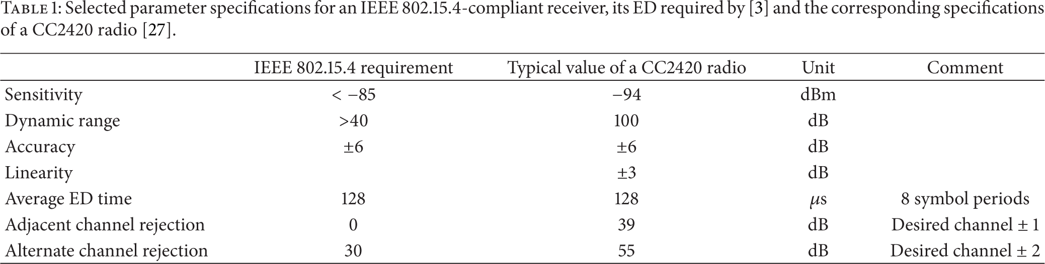
The ED value is better known as RSSI value and is roughly the signal power received at the radio and, therefore, can be treated as power ratio and with the help of an offset of approximately −45 dB [27]; the RSSI value of the CC2420 radio can be roughly mapped to a dBm value indicating the power of the channel.
It has to be mentioned that the signal is measured over an approximately 2 MHz wide channel, as defined by IEEE 802.15.4. Hence, if a signal is narrower than 2 MHz (e.g., Bluetooth), the measured value will be smaller than the signal's peak energy. The RSSI values, which are also the base for the CCA decision, are internally sampled over 8 symbol periods (128 µs), which roughly corresponds to the 8,192 Hz sampling rate (
An implementation detail to collect errorless RSSI readings is that the peak detectors in between the amplifier stages are activated [9]. The interference classification algorithm presented later uses merely binary channel states, namely, clear or busy. The channel state is sampled with the help of the CCA command in default CCA Mode 3 with the preset CCA threshold of −77 dBm at 8,192 MHz.
4.2. IEEE Standard 802.11b, g, n
The IEEE Standard 802.11 with all its different versions is not only various in terms of its modulations (see Table 2) but also very inhomogeneous in terms of traffic and duration of channel access.
Key features of the different versions of IEEE Standard 802.11 operating in the 2.4 GHz frequency band.

DSSS: direct-sequence spread spectrum; OFDM: orthogonal frequency-division multiplexing; DBPSK: differential binary phase shift keying; DQPSK: differential quadrature phase shift keying; BPSK: binary phase shift keying; QPSK: quadrature phase shift keying; QAM: quadrature amplitude modulation; and 1simple channel model.
Features of beacon frames from observed APs. More APs than networks (based on service set identifier (SSID)) mean that the network was built of multiple APs for better coverage.
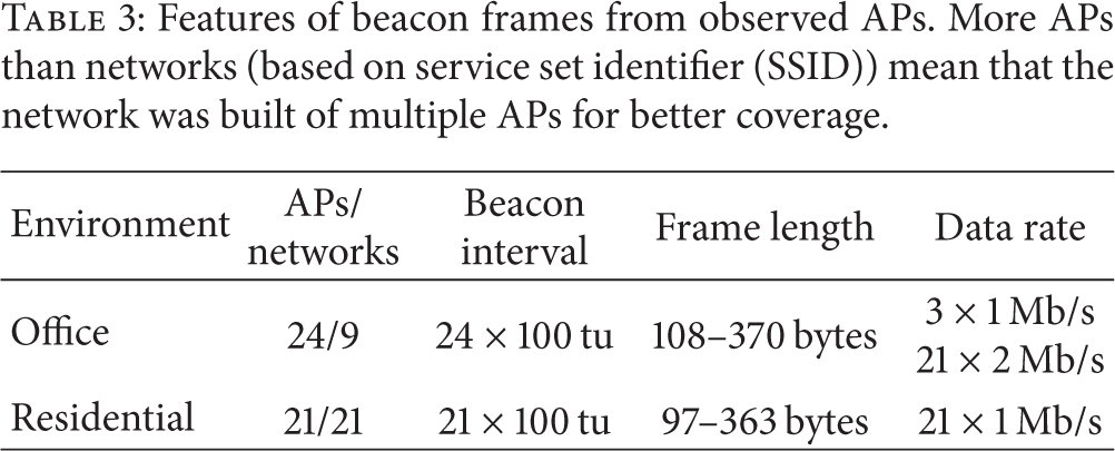
A major feature that is equal throughout different IEEE 802.11 networks is the beacon frame sent by the AP of the WLAN, as also highlighted in [22, 32, 35]. The AP is the central instance, which organizes the network, and, normally, it is also a router that connects a local WLAN to the Internet. The beacon frames are sent periodically by the AP to announce and to maintain the network. However, beacon frames have no reserved time and if the channel is busy due to data traffic the beacon will be delayed and the next beacon will be transmitted according to the original schedule as shown in Figure 9. To provide maximum backward compatibility, the beacon frames are normally sent with the lowest data rate, that is, 1 or 2 Mb/s. The actual minimum airtime of a beacon frame depends mainly on four parts: the preamble (192 μs for the longer PHY Layer convergence protocol (PLCP) header), the MAC header (30 bytes), the cyclic redundancy check (CRC) (4 bytes), and the actual MAC data. Depending on the AP and the network features, the MAC data of a beacon can differ in size. Assuming that a beacon frame has only 50 bytes of payload and is sent with a data rate of 2 Mb/s, an airtime of roughly 0.2 ms can be taken as minimum. Ansari et al. state a minimum time of 0.224 ms [32], while Zhou et al. claim the minimum airtime of beacon frames to be 0.256 ms [22]. These are time durations that can be measured with a sample rate of 8,192 Hz, which is used in the following. See Table 3 for an example of typical beacon properties. Although this table is showing a limited data set, it gives a typical example for real-world WLAN deployments. Based on experience, the authors assume a beacon interval of 100 tu for the rest of this work, since this is the default value, and the authors have not seen any other parameter in deployed networks. The support of a range of beacon intervals increases the computational complexity of the classification and covers only rare special cases. In ad hoc IEEE 802.11 networks (independent basic service set (IBSS)) the master generates beacon frames.
The rest of the IEEE 802.11 traffic varies too much to be used for classification, with many influencing factors as data rate/modulation, numbers of participants, and high-level applications. If the link quality between AP and client changes, the link features for the data traffic, including modulation, can also be altered on the fly. Thus, by using a more reliable modulation, a better link is provided. This adaption is called automatic data rate scaling [42].
Additionally, the RSSI sampling rate of IEEE 802.15.4-compliant radios is not high enough to detect more sophisticated temporal features of IEEE 802.11 as interframe spaces, which would be beneficial for traffic classification.
The channel can be utilized from less than 1% (only beacon frames) up to nearly the whole time (saturated traffic) [43]. An example of an RSSI trace of IEEE 802.11 traffic with easily identifiable beacon frames is shown in Figure 4. It can also be seen that there is a difference between the energy levels of the beacon frames and the data traffic. In this particular setup, the sensor node collecting the RSSI trace was next to the client laptop, while the AP was a few meters away. Nevertheless, by relying on beacon frames only (as most other approaches found in literature [22, 32, 35]), there is the case left of being only under the interference of a client but being outside the range of the AP. However, this case is unlikely, since the AP (mains-operated) normally sends with higher power than the client (often battery-operated). It is not uncommon to have an AP with a transmit power of 17 dBm and a WLAN interface card sending with 15 dBm or less to save power. In theory, four times the power (

Typical RSSI trace of a WLAN. CCA threshold of −77 dBm shown in red. Data collected with the help of [6].
4.3. Bluetooth
Bluetooth uses frequency hopping on the PHY Layer; thus the effect of Bluetooth in a 2 MHz wide IEEE 802.15.4 channel is limited. Three 1 MHz wide Bluetooth channels partly overlay with an IEEE 802.15.4 channel and thereby even permanent channel usage results in
Bluetooth spectrum use due to channel hopping.
Another feature of Bluetooth's architecture is the support of five different logical links or also called logical transport types. The link types used for data traffic can be roughly divided into synchronous links, including synchronous connection-oriented (SCO) and extended synchronous connection-oriented (eSCO) links, and asynchronous connectionless (ACL) links. The SCO links are normally used for voice transfer and are strictly based on single-slot packets, which are not retransmitted in case of a loss. The newer eSCO links are also used for voice transfer, but they support limited retransmissions and their packet lengths are more variable than the SCO packet lengths. The reliable ACL links are packet-based and can use one, three, or five slots. Furthermore, it has to be mentioned that there are two additional link types, the active slave broadcast (ASB) and parked slave broadcast (PSB) links, which are only used for control and network maintenance and are not considered in the following. The link type determines the used packet.
The packet format, modulations, and data rates of Bluetooth are not dealt with in detail, since they are beyond what is measurable with an IEEE 802.15.4-compliant radio. However, the given time slot is a maximum time, which should never be used fully due to guard times. The transmission start time is a clear indicator of Bluetooth communication, because transmissions start with the beginning of a time slot (as shown in Figure 6) and thus time

Timing of single- and multislot Bluetooth packets. Taken from [7].

Typical RSSI traces of a Bluetooth communication. CCA threshold of −77 dBm shown in red. Data collected with the help of [6].
4.4. Microwave Ovens
Although the spectral spread and the power of the leaking radiation differ, all three microwave oven models researched by the authors show similar patterns: the strongest interference occurs on a channel close to IEEE 802.15.4 channel 20, which is around the stated microwave oven center frequency of 2450 MHz (normally the frequency is stated with other device properties on the back side of the oven). The signal is periodic with a frequency around 50 Hz, which is the frequency of the power supply (for North America a frequency around 60 Hz can be expected). In a period of 20 ms, there are an active phase and an inactive phase, which are roughly of the same length. The active phase has two maxima, one at the beginning and one at the end. In between them is a plateau. The height of this plateau differs depending on the oven model, the time, and the channel, but it is generally higher as it is closer to the center frequency. In Figure 8, these timing patterns are shown.

Typical RSSI traces of microwave ovens. CCA threshold of −77 dBm shown in red. Data collected with the help of [6].

Beacon transmission on a busy network. Taken from [8].
Furthermore, microwave ovens have different programs or different power levels that can be chosen by the user. However, the magnetron that emits the microwave radiation can only work at full power. The user-set power level is achieved by pauses between the heating phases. The active and inactive phases of a 50 Hz period are not altered. After a few seconds of heating, a few seconds are given for the heat to spread. This heat spreading times can be easily heard when the microwave oven is not buzzing and when only the ventilation and the turntable operate.
4.5. Classification Algorithm
As already explained, an IEEE 802.15.4-compliant radio has with the help of the ED the chance to detect the increased power in its channels caused by signals; the radio chip does not demodulate. The algorithm presented here collects data with the help of CCA requests, which return binary decisions if the channel is idle or busy, at a sampling rate of 8,192 Hz. A CCA request is performed faster than an RSSI request and therefore leaves more time to process the returned result in between the sampling. Thus, the sample can be analyzed immediately and if a class criterion is fulfilled, the algorithm ends before the maximum runtime of a second and energy can be conserved or a suitable interference mitigation strategy can be applied. The class decision criteria are based on the timing pattern of the channel access and occupation duration of the different technologies. The features computed while sampling can be split into three main groups.
4.5.1. Simple Features
Simple features, which are maxima or sums, can be easily computed and are listed in the following:
the maximum continuous time duration in which the channel was busy
the maximum continuous time duration in which the channel was idle
the channel utilization
4.5.2. Transmission Start Patterns
Transmission start patterns are based on the duration between two rising edges (idle to busy channel transitions). If the time between two successive rising edges is a multiple of the Bluetooth slot time (625 μs), it is assumed to be a Bluetooth pattern. The fits and the misfits are counted as Bluetooth slot patterns
Since the sampling time of 1/8192 s is not an integer multiple of the Bluetooth slot time of 625 μs, the duration computation has been implemented in fixed-point arithmetic.
4.5.3. Periodicity
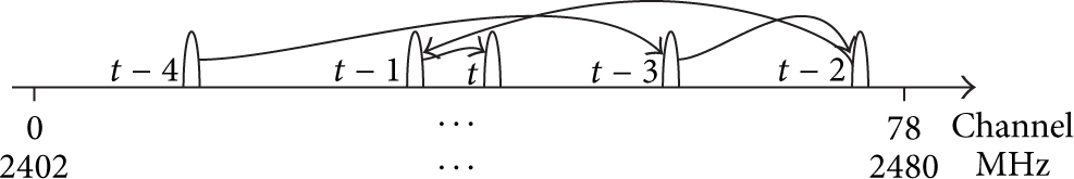
The periodicity (periodicity), which is a function returning a metric p, here, is computed by a simple algorithm to check whether an input signal (signal) is periodic. Due to the limited memory and computing power of sensor nodes, a simple approach to find the frequency component for a binary signal has been selected. It is based on correlation and finds a frequency component, since a signal or function is periodic when
Concept of a simple algorithm to detect periodicity/frequency component p in a discrete, binary signal signal for a given period T given in samples. Further, buffer is a temporal array of the length T.
These features are calculated and checked while the sampling of CCA request values is running. The basic conditions for each class are shown in Algorithm 1. In Algorithm 1 and in the following, the classes of the algorithm are referred to with short labels: CLEAR for no interference, BT1 for Bluetooth single-slot packets, BT2 for multislot packets, WLAN for IEEE 802.11-based WLANs, MWO for microwave ovens, and UNKNOWN for a source of inference that is not known. The algorithm has a further result called INTERNAL, which is returned if the sensor node receives a packet while performing the interference classification algorithm. However, the INTERNAL class is not a classification result but is more an interruption of the classification process. Therefore, it does not appear in the following test results and its use depends on the final application of the classification algorithm.
4.6. Algorithm Timing
An important requirement is to receive an immediate result from the algorithm, since the communication between the nodes of a WSN can be reconfigured faster and energy can be saved. The maximum algorithm execution (radio on) time is one second, which is needed to detect Bluetooth (BT1, BT2) or a clear channel (CLEAR). The channel hopping of Bluetooth leads to little channel use and thus more time is needed to collect enough data for a reliable decision. Other decisions can be made quicker. Especially the microwave oven class (MWO), which is unique in using the channel heavily with a high frequency, can be classified in less time. For a reliable classification, this algorithm relies on a 50 Hz periodicity greater than 15, which means that, after 16 completed periods, a sample can fulfill the requirements, resulting in a

Flow and timing of the algorithm: the gray parts show the time windows when different classes can be detected and the algorithm can return before the maximum execution time.
The algorithm presented here has the advantage that the node is connected to the network all the time and, therefore, it still can receive messages if the interference is not too heavy. Nevertheless, when a message is received in the sampling process, the algorithm is stopped and the INTERNAL class is returned, since the received message also affects the CCA sampling. The problem of internal interference can be solved by an explicit sampling phase for the network coordinated by a central manager as it is suggested in [2] for interference reporting and resolution. The final application of the presented interference classification algorithm is beyond the scope of this work. However, as already mentioned in the literature review (see Section 3), there are multiple applications for the interference classification algorithm (e.g., effective interference mitigation [11, 19–21] or deployment planing [19]) or for parts of it (e.g., low power WLAN detection [22]).
5. Algorithm Testing
An extensive measurement campaign was conducted to test the algorithm: at first, it was tested with selected devices and reproducible data traffic in a controlled environment, that is, a radio frequency anechoic chamber (shown in Figure 12(b)). Secondly, the algorithm was tested in a real-world scenario. The implementation of the algorithm used here classifies a channel three times successively and then changes to the next, higher channel. After channel 26 is classified three times, the classification restarts at channel 11. The INTERNAL class was not tested, since it is not a classification result but is more an interruption of the classification process. Therefore, it does not appear in the following results. The hardware used in the following experiments is listed in detail in Table 4. In the following, it is referred to as the device names given in the first column (for instance, when the word Laptop is used starting with an upper case letter, it stands for the model Dell Latitude E6400).
Equipment used in the course of this work.
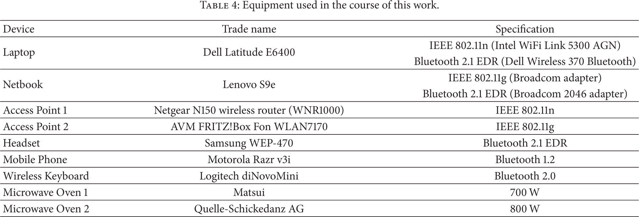
EDR:enhanced data rate.

Experiment setup.
5.1. Controlled Environment
In the controlled environment, a radio frequency anechoic chamber, experiments with reproducible traffic patterns were conducted. First the WLAN classification is tested, starting with high channel utilization (i.e., low data rate traffic), which makes the beacon frames sent by the AP harder to distinguish from the rest of the traffic. The medium channel utilization used next might have similarities to the pattern generated by microwave ovens. Then, a less utilized channel is researched (i.e., high data rate traffic), where the beacon frames stand out more, but the modulation schemes change between beacon frames and data traffic. For this, the channel utilization might be so low that a misclassification as BT2 could happen.
The next batch of experiments deals with the classification of Bluetooth, where the unexpected, irregular channel selection of the Laptop is uncovered. Additionally, a real WLAN and a mixed environment of IEEE 802.11 and Bluetooth are tested.
Finally, the detection of the MWO class is evaluated.
5.1.1. IEEE Standard 802.11b, g, and n
The IEEE Standard 802.11 affects at least four IEEE 802.15.4 channels (see Figure 1). The setup shown in Figure 12(a) was used to test the presented algorithm's ability to classify IEEE 802.11 interference. The interferers, Access Point 1 and the Laptop, were placed 4 m away from each other. Three Tmote Sky sensor nodes running the interference classification algorithm were placed in the middle between Access Point 1 and the Laptop. The Netbook that generated the data was connected to Access Point 1 via Ethernet, which then transmitted the data to the Laptop via IEEE 802.11. The WLAN traffic patterns generated to test the algorithm are described in the following.
Heavy Channel Utilization. To get an idea on how the algorithm reacts under heavy channel loads, the tool JPerf 2.0.2 [44] was used. The heaviest congestion on the channel was generated using the slowest data rate, that is, IEEE 802.11b. Note that, although higher data rates are often supported by today's hardware, the link can fall back to a lower data rate (as used in IEEE 802.11b) in bad radio frequency conditions due to automatic data rate scaling (see Section 4.2). Furthermore, with higher data rates, the theoretical, maximum channel utilization decreases [43]. With high channel utilization the actual beacon frames sent by the AP are less outstanding from the data traffic.
In the WLAN that was used here, the beacon frames sent by Access Point 1 had a length of 196 bytes at a data rate of 1 Mb/s and were sent at the default, preset interval of 102.4 ms. The communication between the two IEEE 802.11b communication partners took place on channel 11, which overlaps with the IEEE 802.15.4 channels 21, 22, 23, and 24. The theoretical maximal data rate is 11 Mb/s. In the setup used here, a throughput of up to roughly 5,800 kbit/s was achieved. The test included TCP and UDP connections. The window sizes for TCP were 56, 1,000, and 2,000 KBytes. The window size has an effect on the number of acknowledgments and therefore tunes the channel utilization. With fewer acknowledgments, fewer responses from the network partner have to be transmitted. Additionally, each test was run in a unidirectional, dual (i.e., alternating directions) and trade (i.e., at first in one direction, then in the other) mode. For UDP traffic a 1 MB/s and a 10 MB/s bandwidth links were used, where the second setup saturated the channel. This led to a maximum airtime-based channel utilization of up to 99.44% over one second on IEEE 802.15.4 channel 22 measured by the Tmote Sky sensor node. This measured channel utilization is greater than the given theoretical maximum in [43], but the ED-based measurements of the Tmote Sky are not fast enough to reflect the channel utilization fully correct.
Eleven different IEEE 802.11b data traffic settings were used in total, which resulted in 300 classifications (composition: 24
The classification of IEEE 802.11 on the four fully overlapping channels achieved very good rates, always greater than 95.33% with an average of 99.58%.
However, the adjacent channels 20 and 25 suffered from misclassifications and were only classified with 62.00% and 28.67% as CLEAR. These two channels were mainly classified as UNKNOWN, which can be explained as follows. The data traffic and the beacon frames have different modulation schemes even within the IEEE 802.11b standard. The beacon frames, sent with 1 Mbit/s, use baseband modulation of DBPSK and the data traffic, sent with 11 Mbit/s, uses the so-called “higher rate” 8-chip complementary code keying (CCK) modulation scheme [8]. Table 2 shows the different modulations of different standard versions. Vanheel et al. [45] report similar observations, claiming that OFDM has a wider spectrum than DSSS. This effect will become clearer in the following experiments (see Table 5). Due to the close proximity owing to the limited physical dimensions of the radio frequency anechoic chamber, the effect of the different keyings/modulations observed here is worse than in most real-world setups with greater distances between the devices. With greater distance between the IEEE 802.15.4 node and the IEEE 802.11 device, the out-of-band energy of the latter is decreased and thus the problem of misclassification on adjacent channels is minimized. This decrease can be seen in Table 10 showing the results of a setup in which Access Point 2 is farther away from the node in an uncontrolled environment.
Controlled environment IEEE 802.11 experiments for low channel utilization summarized by channels. Classification results (%) of 78 classifications for each channel for different IEEE 802.11 versions. Low IEEE 802.11 traffic generated by D-ITG. The given result is the mean of three nodes and the standard deviation between nodes is in parentheses.

Also, the variance between the nodes was very high on the adjacent channels. This is due to the fact that the nodes were not synchronized. Therefore, the nodes might have slightly different sampling windows in time.
The rest of the channels which should not be affected by IEEE 802.11 were classified almost always correctly as CLEAR. The few misclassifications, decreasing with more distance of the WLAN center frequency, can only be explained due to out-off-band emissions of the IEEE 802.11 devices or erroneous CCA readings.
Medium Channel Utilization. To evaluate the algorithm for medium channel utilization, different traffic patterns were used as suggested in [46]. The IEEE 802.11b traffic was generated by D-ITG [47], while the hardware and spatial setup stayed the same. Rates of 500, 250, 90, 45, and 9 TCP packets per second, each 1500 bytes long, were sent, resulting in theoretical data rates of 6000, 3000, 1080, 540, and 108 kbit/s, respectively. Whereas the rate of 6000 kbit/s has not been achieved in our setup, only a rate of 4009 kbit/s could be measured, which is an acceptable performance for an IEEE 802.11b network (taking into consideration that the latter has only a theoretical data rate of 11 Mbit/s). For all three Tmote Sky sensor nodes in all five test cases, the classification of WLAN worked flawlessly on channels 21, 22, 23, and 24. Only a single experiment on a single node had a classification rate below 100% being an outlier with 83.33%. This results in 98.89% of correctly classified channels 21, 22, 23, and 24 over all experiments. The adjacent channels, 20 and 25, showed the same problem as described in the previous experiment.
Low Channel Utilization. To investigate low channel utilization (<10%) further experiments with D-ITG generated traffic were conducted: 10 min of random data traffic have been sent from the Access Point 1 to the Laptop (uniformly distributed packet rate: 1 to 1000 packets per second and uniformly distributed packet size between 1 and 1000 bytes for TCP and UDP).
A summary of the results is shown in Table 5(a) to Table 5(d). The results in the tables are averaged over the three classifying nodes and broken down into channels. The detection results on the four mainly affected channels are very good, only in the IEEE 802.11n experiment (see Table 5(c)); a node struggled for the TCP experiment on channel 21 for an unknown reason, dragging the average classification rate down and increasing the standard deviation given in parentheses. For 22 MHz wide channels, the already discussed phenomena of misclassifications on adjacent channels occurred for all versions of IEEE 802.11. Table 5(d) shows another difficulty regarding IEEE 802.11n using the 40 MHz wide channel bonding. Besides the fact that the 40 MHz wide channel jams almost all the available frequencies, including, for example, the orthogonal IEEE 802.15.4 channel 20 (see Figure 1), the second channel cannot be identified by this algorithm. This is due to the fact that the second IEEE 802.11n channel is not used for beacon frames and actually is only connected for the data exchange between communication partners. The issue of the secondary channel of a 40 MHz wide IEEE 802.11n channel bonding is very challenging and, to the best of the authors’ knowledge, it has not found greater recognition in the WSNs community yet and remains an open research question.
Real-World Channel Utilization. Additional to the artificially generated data traffic, the algorithm was tested in a more realistic setup in the radio frequency anechoic chamber. Two clients were connected to the Access Point 1: the Netbook was connected with an IEEE 802.11g (54 Mbit/s) connection and the Laptop with an IEEE 802.11n connection using a single channel (72 Mbit/s). Both clients streamed a video. The spatial setup, which is shown in Figure 13, was as follows: the Access Point 1 was placed 1.20 m above the ground, while the Netbook was placed 3 m and the Laptop was placed 5 m in distance to the Access Point 1 on the ground. The sensor nodes were spread between the Netbook and the Laptop. The classification results were again compelling, as can be seen in Table 6, showing that the data traffic had no influence on the reliability of the AP classification. However, again, on channel 21, the results vary mostly between the nodes. The out-off-band energy leading to misclassifications on adjacent channels increased slightly, since the sensor node was very close to the clients, which also transmit to the AP.
Controlled environment IEEE 802.11 experiments for real-world utilization summarized by channels. Classification results (%) of 57 classifications for each channel. IEEE 802.11 video streaming with two clients (mainly overlapping channels 21–24 are bold). The given result is the mean of three nodes and the standard deviation between nodes is in parentheses.

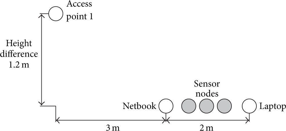
Setup of the experiment “real-world channel utilization.”
5.1.2. Bluetooth
The classification quality of Bluetooth was evaluated in multiple experiments. The distance between the two Bluetooth communication partners was 4 m in all experiments described in the following. The sensor nodes were placed in the middle between them, as shown in Figure 12(a). The traffic of the Bluetooth connection was monitored on the L2CAP Layer with hcidump [48] on the Laptop running Linux. The L2CAP Layer roughly corresponds to the Data Link Layer of the OSI Reference Model. The Netbook used Windows XP as an operating system.
In the first experiment, an audio file was streamed from the Laptop to the Headset. The stream was based on eSCO links with 60 information bytes packed into an extended voice (EV) packet sent with an EDR. The resulting packets stayed in the time limitation under 625 μs. Hence, the according algorithm return is BT1; the results are shown in the row “Laptop to Headset (eSCO)” in Table 7(a). The second experiment “Netbook to Headset (eSCO)” was equal to the previous, but this time the Netbook was used instead of the Laptop.
Controlled environment Bluetooth experiments summarized by experiments and details of experiment with the worst classification rate.

The third experiment was a data transfer from the Laptop to the Mobile Phone. This experiment was followed by a transfer in the opposite direction. The experiments are shown in the rows “Laptop to Mobile (ACL)” and “Mobile to Laptop (ACL).” Again, these two experiments have been repeated with the Netbook instead of the Laptop. Finally, the data was transferred between the Laptop and the Netbook, with the Netbook supporting a newer version of Bluetooth than the Mobile Phone and, hence, the transfer was different from the one in the previous setup. Again, both directions were tested and are shown in Table 7(a).
Although Table 7(a) merely shows the example results of a single node for better clarity, the results of other nodes did not vary significantly. Since the results are already averaged over 16 channels, only a single node with no standard deviation is presented. However, for cases with a high variance between different channels, it is discussed in the following.
The eSCO packets were classified well in Experiment 1. In Table 7(a), the sum over all channels is shown for the experiment, but a detailed view reveals that most channels had a 100% classification rate, while other channels had a lower rate (down to 69.23%). On these channels, the traffic was misclassified as UNKNOWN. Experiment 2 reaches a nearly 100% classification rate. The channels in Experiment 2 are more equally used as by the Laptop. The phenomenon of the unequal channels for all connections with the Laptop occurs in all the following experiments.
In the remaining experiments, ACL packets were transmitted, using one, three, or five time slots and, hence, making the traffic more difficult to identify. However, as shown in Table 7(a), the classification rates were still satisfactory. Note that almost no misclassifications as WLAN and no MWO misclassifications were made.
When the Laptop was used as sender, some channels were unused. The worst case, occurring in the experiment “Laptop to Netbook (ACL),” is shown in more detail in Table 7(b). Channels 14, 15, 16, 17, 21, and 25 are idle, classified as CLEAR, most of the time. Since the authors used off-the-shelf hardware and driver software, the reason for this is not fully clear. Although the Wi-Fi card of the Laptop was deactivated during the experiments, a WLAN-Bluetooth coexistence mechanism possibly could have blocked channels. The Netbook-based connections show more uniform spread results with all channels being equally, correctly classified (with
It could be argued that a longer classification time improves the results of the algorithm, but, from a theoretical point of view, this is unnecessary. A time slot, which is normally the time the frequency is kept, is
The last IEEE 802.11 experiment, “real-world channel utilization,” was redone with an additional Bluetooth audio link generating eSCO traffic. The video streaming Laptop client used the Bluetooth Headset to listen to the sound. All other setup properties, including the Netbook, stayed the same. The WLAN was already established and used when the Bluetooth connection was established and thus the AFH mechanism or the method used by the Laptop to choose the channel for Bluetooth had enough time to adapt its channel choice before the classification was started. The results are shown in Table 8 and attest the expected behavior: Bluetooth is not detected on the channels used by IEEE 802.11 (21, 22, 23, and 24). This behavior is expected since the IEEE 802.11 frequencies are blacklisted by Bluetooth due to the used AFH. AFH works as follows: After each transmission, the channel changes according to a pseudorandom pattern. If the transmission fails on a channel, AFH will avoid using this channel for a predefined time. If AFH had not been used, the WLAN traffic would dominate on the overlapping channels, which would make the Bluetooth traffic hard to detect.
Controlled environment IEEE 802.11 and Bluetooth experiment summarized by channels. Classification results (%) of 57 classifications for each channel. IEEE 802.11 video streaming with two clients, Bluetooth audio streaming (eSCO) from the Laptop to the Headset (expected classifications are bold). The given result is the mean of three nodes and the standard deviation between nodes is in parentheses.

5.1.3. Microwave Ovens
To test the classification rate of the algorithm for microwave ovens, 500 mL of water in a plastic bowl were placed inside Microwave Oven 1 and heated with full power for 5 minutes. In front of the microwave, nodes were placed 0.5 m, 1.0 m, 1.5 m, and 2 m away. The classification results of the most affected channels (18, 19, 20, and 21) are shown in Table 9(a). These channels around the center frequency of the microwave oven were classified mainly correctly.
Controlled environment microwave oven experiment summarized by distance and details of node closest to the oven.

Uncontrolled environment IEEE 802.11 experiments summarized by channels. Classification results (%) of 51 classifications per channel for low, real-world IEEE 802.11 traffic (mainly overlapping channels 11–14 are bold). The given result presents the mean of three nodes and the standard deviation between nodes in parentheses.

As for IEEE 802.11, channels farther away from the center frequency of the interferer are much harder to classify since they do not suffer from the typical interference pattern but from harmonics. Table 9(b) shows the results of 18 full spectrum sweeps for the 0.5 m setup, where the node was closest to the microwave. On channels farther away from the center frequency, it might happen that the energy is just around the CCA threshold and only very few CCA requests report a busy channel, which can be mistaken with Bluetooth, since 50 Hz are a divisor of 1600 Hz.
5.2. Uncontrolled Environment
In addition to the tests in the radio frequency anechoic chamber, which delivered results from an ideal environment, tests were also conducted in a detached house. This added effects as reflections and multipath propagation to the setup. Additionally, the devices used in these experiments have not been part of any training set used to develop the algorithm. Therefore, the following tests can be considered to be challenging and far beyond the testing reported for the reviewed algorithms in Section 3.
5.2.1. IEEE Standard 802.11g
Access Point 2 was in another room on the second floor; thus the received signal was around −50 dBm at the Laptop next to the sensor nodes on the first floor. The distance between the two devices was around 10 m on the plane and roughly 2.50 m in height with multiple rooms between them. The beacon frames were sent in the default interval of 100 tu at a data rate of 1 Mbit/s and were 189 bytes long. The classification algorithm ran for 10 min, resulting in 51 full channel sweeps. For further details, see Table 10. Since IEEE 802.11g used channel 1, the IEEE 802.15.4 channels 11, 12, 13, and 14 were supposed to be affected. There was notably less misclassification on adjacent channels, which is due to the fact that the power spectral density (PSD) of the beacon frames sent with a low data rate modulation has a distinct maximum at the center frequency. Furthermore, the distance and, therefore, the attenuation in this scenario were much higher than in the measurements in the controlled environment (see Section 5.1.1). Even channels 11 and 14, which are fully overlapped by the 22 MHz wide IEEE 802.11 channel were less interfered and thus less often classified as WLAN.
5.2.2. Bluetooth
To evaluate the Bluetooth classification rate, again, a new untested device was used: the Wireless Keyboard was connected to the Laptop and placed on the same table as the sensor nodes and the Laptop. The classification ran for 10 min resulting in 45 full channel sweeps. The test results were acceptable: over all 16 channels, the
5.2.3. Microwave Ovens
For this experiment, Microwave Oven 2 was used to heat 500 mL of water in a plastic bowl for 5 min and the sensor nodes were placed 0.5 m away from the front side of the oven. As it can be seen in Table 11, the classification results were only modest. The best classification rate was achieved on channel 23 (center frequency of 2465 MHz), while channel 20 (2450 MHz) was expected.
Uncontrolled environment microwave oven summarized by channel. Classification results (%) of 21 classifications per channel 0.5 m away from Microwave Oven 2 in an uncontrolled residential environment. The given result presents the mean of three nodes and the standard deviation between nodes is in parentheses. For a better evaluation, the measured channel utilization

However, these results reflect what the channel utilization
5.2.4. Long-Term IEEE Standard 802.11g
Since all experiments described so far were limited in time duration, a 24-hour long-term experiment was conducted in the same residential environment as all the uncontrolled environment experiments in this section. The channel sweep was timed to start every two minutes and a channel classification started every two seconds, with three classifications on the same channel before the channel was changed. Thus, the early returns did not affect the timing and 720 full channel sweeps were performed resulting in 2,160 classifications per channel.
Access Point 2 was operating on IEEE 802.11 channel 6, which overlaps with IEEE 802.15.4 channels 16, 17, 18, and 19. During the experiment, multiple laptops, a desktop computer, and a smartphone have been active as clients. Additionally, Bluetooth traffic was generated by the Wireless Keyboard, which was connected to a generic Bluetooth dongle plugged into the desktop computer.
This experiment generated a trace of the algorithm output over a long time. However, since this experiment was performed in a live environment, there is no ground truth data. Therefore, only the results for the WLAN class can be evaluated, since the WLAN was, as in common practice, permanently announced. The Wireless Keyboard was just used during a time span in the evening. The WLAN classification worked reliably with 99.7222%, 99.5833%, 99.4907%, and 99.3056% correct classifications on channel 16 to 19.
In Figure 14(a), the channel utilization is shown, which is commonly used to categorize channels (e.g., in [2]). When Figures 14(a) and 14(b) are compared, it can be seen that the presented classification algorithm delivers much more information than the simple channel utilization. Due to the beacon detection, a WLAN is detected as a possible source of interference, although it might be idle at the moment and the IEEE 802.11 channel is not used. A simple threshold of the channel utilization cannot detect IEEE 802.11 for most of the time and, therefore, channels 16, 17, 18, and 19 would be considered as good choices. In the late evening from 22:30 to 23:30, the channels are under heavy interference, because the WLAN was used by multiple clients. In this case, an earlier detection and avoidance of the IEEE 802.11 channels would prevent interference, which would lead to a channel change. Thus, especially the detection of IEEE 802.11 is useful for a long-term channel planning. Since the algorithm also measures the channel utilization internally, the resulting class can be further judged by the actual medium use. This example shows the potential of the presented algorithm for real-world WSN deployments.
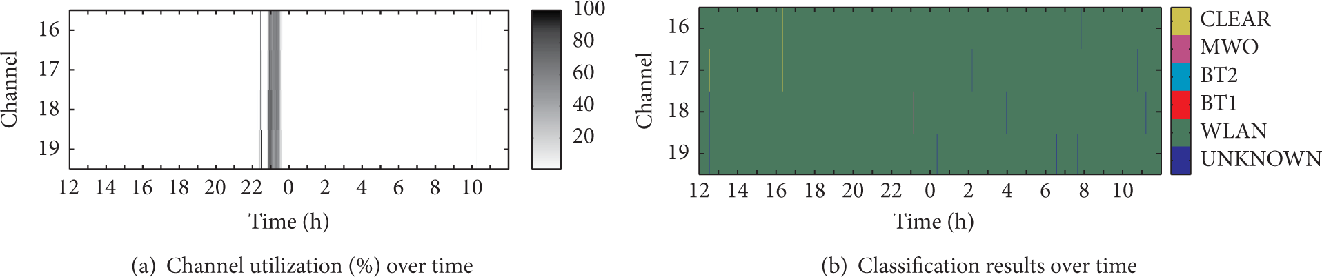
Results of a 24-hour long-term evaluation of the classification algorithm in a real-world environment (trace of a single node).
6. Results and Discussion
In this work, an algorithm is introduced to classify one second or, in most cases, a shorter trace of CCA samples into one of six classes, namely, idle channel (CLEAR), Bluetooth single-slot packets (BT1), Bluetooth multislot packets (BT2), IEEE 802.11-based WLANs (WLAN), microwave ovens (MWO), or an unknown source of interference (UNKNOWN). If the classification is interrupted by receiving an IEEE 802.15.4 packet, the classification of the source of interference is not finalized and the INTERNAL class is returned. Furthermore, the algorithm classes and the algorithm implementation are described and, finally, the algorithm was tested in multiple scenarios. In the following, the test results are discussed and compared to the state-of-the-art.
6.1. Classification Results
The extensive testing of the algorithm conducted in the previous section allows the following conclusion of the classification performance: The WLAN classification worked well for 22 MHz wide channels. The phenomena that adjacent channels were often interfered but misclassified can, as already mentioned, be explained with the different modulations and the close distance. Due to the different modulations, the data traffic might still affect an IEEE 802.15.4 channel, on which the beacon frames are received below the CCA limit. Nevertheless, the experiments also showed that the data traffic in the WLAN has little to no effect on the classification rate.
The Bluetooth classification here represented by two classes BT1 and BT2 works satisfactorily. On the used Laptop, some channels were avoided, which decreased the overall classification rate. However, if a channel is not used by Bluetooth, it cannot be classified as such; thus, the sometimes low classification rate is a pessimistic measure. Also, Bluetooth interferes only very little on a single IEEE 802.15.4 channel and therefore there is little to measure.
The MWO class delivered only moderate classification results, especially in the uncontrolled environment. Since microwave ovens have no standards nor specifications for the emission of radiation as communication technologies have, this problem is not fully solvable, although in countries with a different electrical system providing a different frequency, for example, North America, the algorithm has to be slightly adapted.
To give an overall classification rate or a comparison to methods suggested in literature is difficult, since multiple factors influence the classification rate, including traffic/modulation of interferer, spectral overlap, distance, and CCA threshold. However, the reported rates and the test setups are shortly reviewed in the following to provide a rough possibility of comparison.
Zhou et al. [22] evaluate their AP beacon detection with four different APs and traffic generated by D-ITG. Additionally, they check their approach for cross-sensitivity with IEEE 802.15.4 traffic. They report a detection rate of 95%; the frequency offset is not mentioned, but the runtime of the algorithm is given. If only the two IEEE 802.15.4 channels next to the center frequency of the used IEEE 802.11 AP are used, the algorithm presented here has a higher detection rate in the controlled environment and a comparable rate in the uncontrolled environment.
Chowdhury and Akyildiz [19] evaluate their approach with simulations and do not state a classification rate for IEEE 802.11 or microwave ovens. Similarly no statement is made by Bloessl et al. [31] and Nicolas and Marot [21].
Ansari et al. [32] state a 96% detection rate of IEEE 802.11, but they only detect a single class in a near-ideal environment without any cross-sensitivity or control group.
The publications of Hermans et al. [33], Rensfelt et al. [11], and Hermans et al. [20] developing SoNIC are the most comparable to the algorithm presented here and since the latter publication is the most recent and best evaluated one, the authors will refer to it. Hermans et al. [20] claim to detect the predominant source of interference in an office environment with 87%. However, confusion matrices given in their work show that especially the IEEE 802.11 detection is relatively low with 82.0%. Due to unclear frequency offsets and different devices used, the rates cannot be directly compared to the work presented here. As already mentioned in Section 3, the algorithm presented here is, to the best of the authors’ knowledge, the only one distinguishing between single-slot (BT1) and multislot (BT2) Bluetooth packets. The authors believe that the Bluetooth packet length has effects on the pattern of the corrupted bits. Further, it is not only the varying airtime of Bluetooth, but also the modulation change within Bluetooth packets of higher data rate [7].
Additionally, the detection of bonded channels used by IEEE 802.11n has not been discussed in literature yet.
A common limit is that only a single, at least per channel, source of interference can be detected. Airshark [24] can detect multiple interferers at once. However, due to the used IEEE 802.11-based hardware and a computer for its computations, Airshark has more possibilities compared to those approaches which are based on IEEE 802.15.4-compliant radios and microcontrollers. Due to the inability of IEEE 802.15.4 radios to demodulate signals and the blurry ED, this limit is very challenging to overcome. Nevertheless, in the unlikely case of different interferers overlapping in frequency, the approach presented here only detects the source with the highest channel utilization. This is also equal to the timing of decisions (see Figure 11): Microwave ovens (which do not back off for other participants), IEEE 802.11, and then Bluetooth (being the weakest technology with inbuilt external interference avoidance with the help of AFH).
In SoNIC [11, 20], a weak IEEE 802.15.4 link is an additional class, but the approach presented here using ED instead of corrupted bits makes the distinction easy, since, for weak links, there is no high background noise level generated by external interferers. This work focuses on external interference in the 2.4 GHz frequency band and therefore weak signals due to long distances between the nodes were not considered.
Another influencing factor is internal interference. Since the algorithm presented here can still receive packets, it can react to traffic within its WSN. However, the CCA trace is influenced due to the IEEE 802.15.4 traffic and the algorithm represents the packet reception with the help of the INTERNAL pseudoclass. Depending on the use of the classification, the INTERNAL result might lead to a restart of the algorithm.
6.2. Execution Time
Besides the classification rate, which should be as high as possible, for example, to prevent the decision for an unsuitable mitigation strategy, the execution time is a vital feature of interference classification. The execution time, that is, the time after which enough samples have been collected to end the algorithm and return a result, is important to adapt the communication as fast as possible. For most experiments conducted, it has been close to the theoretical minimum. In theory, at least 5040 samples (
7. Conclusions
This work gives an overview of the situation of the crowded, license-free 2.4 GHz ISM frequency band and the related literature is reviewed. It introduces the most common technologies operating at this frequency, starting with IEEE 802.15.4 and showing its possibilities to detect signal energy with IEEE 802.15.4-compliant radios. This ED allows detecting external sources of interference, which are, namely, IEEE 802.11-based WLANs, Bluetooth, and microwave ovens. These technologies are presented with a focus on their airtimes. After introducing these preliminaries, an algorithm is developed and examined and its implementation is thoroughly tested. This shows that the classification rates are competitive and that more classes are supported compared to most other approaches. Furthermore, the testing of the implementation is beyond what is commonly found in literature, including tests in a radio frequency anechoic chamber and in a real-world setup, different traffic patterns, and various versions of IEEE 802.11 (while IEEE 802.11b is still dominant in literature). Bluetooth has been subdivided into single- and multislot traffic and has been tested in different versions. Even the combination of IEEE 802.11 and Bluetooth has been researched, showing that returning a single class is not a drawback of the algorithm. This is due to the facts that it returns the main source of interference on the channel and that Bluetooth avoids channels used by IEEE 802.11 on its own with the help of AFH. However, the deep testing of the algorithm unveiled the problem of detecting 40 MHz wide bonded channels supported by IEEE 802.11n. This remains as an open task for future versions of the algorithm. The algorithm can also be extended to classify more technologies operating in the 2.4 GHz frequency band.
Finally, the classification result of a channel not only is informative but also can be used to adapt the transmit parameters (as, e.g., in [5, 11, 19, 21, 49]). Thus, an interference-aware communication protocol that adapts its parameters to the class of interference is a potential application for this algorithm. Therefore, interference caused by and classified as IEEE 802.11 could be mitigated with the help of a channel change as suggested in [11, 20, 21]. Interference caused by microwave ovens could be overcome by packet scheduling (as suggested in [11]) or by a channel change, which results in more overhead than packet scheduling, especially in large WSNs. However, interference mitigation strategies as well as other potential applications, for example, deployment planning (as in [19]) or a low power preswitch for IEEE 802.11 network interface cards (as in [22]), are beyond the scope of this work and remain for further research in the near future.
Footnotes
Conflict of Interests
The authors declare that there is no conflict of interests regarding the publication of this paper.
Acknowledgment
The authors wish to thank the following for their financial support: The Embark Initiative (IRCSET) and Intel, which funded this research, and Cost Action TD1001 for additional support.