Dimensional Accuracy Enhancement in CNC Batch Grinding through Fractional Order Iterative Learning Compensation

Abstract

This paper presents a systematic method to compensate for dimensional errors of workpieces machined in computer numerical control (CNC) batch grinding process. The dimensional error precompensation scheme includes a fractional order compensator, automatic dimensional measuring device, and a comparator. A practical fractional order differential plus low-pass iterative learning approach is used to update the compensation for the next workpiece. An incremental order updating law is proposed for the fractional system order identification, which plays a fundamental role to optimize the performance of grinding process. Then the error compensated numerical control (NC) program is fed to the machine tool for subsequent grinding. Several illustrated results show the effectiveness of the above strategy.

1. Introduction

The role of batch processing is ever-increasing in today's diversified manufacturing environment. Besides the fine or specialty chemicals, computer numerical control (CNC) precision grinding occupies an important position in batch production. The machine tools may operate continuously for several days grinding hundreds or even thousands of parts. Since there exist several error sources, such as geometric and kinematic errors of machine tools, thermal errors, cutting-force induced errors, and other errors [1], as well as the properties of workpiece and grinding wheel, the dimensional error is presented nonlinearly and nonmonotonously. As the growing demand of precision components and consistency of quality, it is especially important and rigorous to control the dimensional accuracy of workpieces within the accepted error tolerance.

In general, the surface dimensional error is induced mainly by the deflection of the tool and the workpiece during grinding, which does not remove the material as planned [2]. The strategies to reduce the errors that adversely affect the accuracy of workpieces can broadly be divided into two categories, namely, error avoidance and error compensation. The general approach towards building an accurate machine tool is to apply error avoidance techniques during its design and manufacturing stage so that the sources of inaccuracy are kept to a minimum. However, such machines also tend to be overdesigned and too expensive. Unlike the case of error avoidance, error compensation is a cost-effective way of improving accuracy without any significant changes to the configurations of the machines.

As known to all, the required error corrections can be calculated by measuring various process variables and utilizing the models for various error components or directly from the measurements made on the machined part. The machining error compensation can be affected using the on-line (direct) or the off-line (indirect) method.

The on-line methods [3–6] have technical and cost limitations, which cannot be described as a global method for all types of machine tools. The off-line methods [7–11] are generally based on the compensation of geometric error, thermal error, cutting force, and static/quasi-static error.

The main interest of research worldwide in error compensation of machine tools is directed to the question of how to find an accurate mathematical model with the minimum number of sensors detecting different error sources within an acceptable time scale. However, as previously discussed, in CNC grinding the rate at which the dimensional error increases is a function of many factors. As described in [12], the grinding wheel abrasion not only decreases the size of the grinding wheel, but also blunts it. A blunt grinding wheel increases the grinding force and the feed system elastic distortion and, hence, increases the dimensional error of the machined part. Dressing a blunt grinding wheel decreases its size and, hence, increases the piece dimension, unless it is compensated. However, a dressed grinding wheel becomes sharper and tends to decrease the elastic distortion of feed system, which conversely increases the accuracy of the nonlinear grinding process. Up to now, most of the developed mathematic models consider at once no more than three error sources, which cannot compensate for the dimensional error absolutely. And the mathematical model may not adjust automatically with accidental factors.

The authors in [13] proposed an intelligent dimensional error precompensation scheme for entire process without identifying any component. In view of this idea and avoiding the difficulties of custom methods, a fractional order iterative learning compensator is put forward for dimension accuracy enhancement in this paper. Iterative learning control (ILC) [14] has been an intensive research in the past decades. To date, many ILC schemes have been developed and applied in industry in the past decades. For example, an ILC scheme was applied to the batch process in a rapid thermal processing (RTP) system [15]. The basic scheme of ILC is shown in Figure 1, where u _k (t) and y _k (t) are, respectively, the system input and output in the k_th iteration, u_{k + 1}(t) is the system input of the ${(k+\mathrm{1})}_{\text{th}}$ trial, and y _d (t) is the given desired trajectory. The goal of ILC is that lim⁡_{k → ∞}y _k (t) = y _d (t) holds for all t ∈ [0, T], where T is a fixed time constant. The system structure (linear or nonlinear) is known in advance. In fact, ILC theory firstly was focused on nonlinear system, and the algorithms can be applied to nonlinear system satisfying the globally Lipschitz condition. This critical restriction was firstly broken through based on Lyapunov in 1995 and has highly developed in the past decades [16–18]. ILC approaches can achieve perfect tracking performance through repeating the batch process with learning.

Figure 1:

Basic scheme of ILC.

The development of fractional order ILC (FOILC) algorithms belongs to a branch of fractional order control [19–21]. The D^α-type ILC algorithm and its convergence condition are firstly proposed in frequency domain [22]. The time domain analysis of fractional order ILC is shown in [23, 24] and the references therein.

For a nonlinear system and system with uncertain or unknown structure information, the system order is unknown. In this case, applying integer order ILC schemes directly to the controller cannot achieve desired performance. If the system order (α) is obtained through identification in advance, then the α_th-order iterative learning scheme can be introduced to improve the transient and static performance of the system.

This paper proposes a fractional order D^α plus low-pass iterative learning approach to identify the system order and compensate for dimensional errors in CNC batch grinding process. An incremental order updating law is proposed to identify the grinding system order α using the system inputs and outputs without knowledge of other parameters. If α is an integer, then the system is an integer order system. If α is fraction, then the system is a fractional order system. The optimal iterative learning controller for the α_th-order system is also α_th-order one. In order to achieve fast convergence rate and perform conveniently, the D^α plus low-pass iterative learning scheme is introduced. To obtain precise and accurate machined parts, the preprocessing scheme, which starts from analyzing initial NC program and results in error compensated NC code, is implemented. By using this method, no sensor or model is needed. For a batch of the same type workpieces, the dimensional errors can be decreased efficiently.

2. Principle of CNC Grinding and Structure of the Intelligent Compensation System

The structure of the CNC grinding machine tool for grinding workpieces is shown in Figure 2. As shown in Figure 2, the X axis is the feed shaft of the machine tool, which is defined as being parallel to the rotation axis of the grinding wheel. The workpiece is rotated about the C axis. And the B axis is the rotation axis of the workbench, whose center of rotation is the intersection point of X axis and grinding wheel surface. The periphery of the workpiece is machined through a combination of movements along the C, X, and B axes. The B axis rotates for machining complex surfaces.

Figure 2:

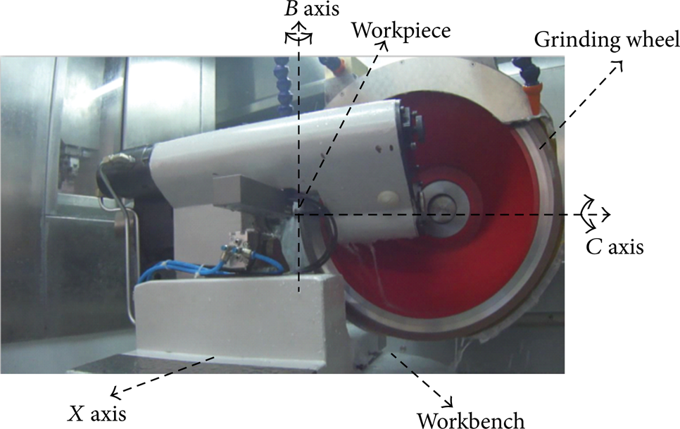
Structure of the machine tool.

Dimensional error compensation of the workpiece is achieved by fine adjustment along the X axis. The block diagram of the CNC grinding system with fractional order iterative learning compensator is shown in Figure 3. The comparator includes two inputs: one is the desired dimension (Dime) determined by NC code and the other is the actual dimension of the processed workpiece (D(k)) measured by an automatic measuring device. Then the resulting error (E(k)) is fed to the fractional order iterative learning compensator, and the compensation is determined by the compensator. Note that k = 1, 2, 3,…, which is the k_th workpiece. The memory is a first-in-first-out stack where the control information relating to previously machined workpiece is stored. The control information includes the measured dimension D(k), the dimensional error E(k), and its compensation value C(k). Based on the control information and reasoning rules, the correction value C(k + 1) for the next workpiece is determined. The controller adds the compensation signals to the coordinates involved in an NC block command and then transfers the modified NC block command to CNC controller. Figure 4 shows the basic concept of error compensation in CNC grinding machine tools. In this way, the dimensional precision of workpiece will be improved continuously.

Figure 3:

Block diagram of the CNC system with fractional order iterative learning compensator.

Figure 4:

Flow chart for the concept of error compensation.

3. Compensation Algorithms

3.1. The D^α-Type ILC Scheme for Fractional Order Nonlinear System

For the nonlinear grinding process in this paper, a fractional order differential plus low-pass ILC scheme is applied to guarantee the convergence and to identify the order of the system. The simplified fractional order nonlinear SISO system in this paper is

$y^{\left(\alpha \right)}\left(t\right)=f\left(u,y,t\right),$

(1)

where α ∈ (0, 1), y(0) ∈ R^{n × 1}, u ∈ R^{m × 1}, ${}^{(\alpha )}$ denotes the α_th-order Caputo derivative [21] with respect to t, and the continuous differentiable function f satisfies the global Lipschitz condition

${\parallel \frac{\partial f}{\partial y}\parallel }_{\infty }\le c{\parallel y\parallel }_{\infty },$

(2)

where c is a Lipschitz constant, c > 0.

The fractional order ILC scheme for dimensional accuracy enhancement is shown as follows:

$u_{k+\mathrm{1}}\left(t\right)=u_k\left(t\right)+K_d\left(t\right)e_k^{\left(\alpha \right)}\left(t\right),$

(3)

where α ∈ (0, 1), K _d (t) is the gain function, k = 0, 1, 2,…, t ∈ [0, T], and y _k (0) = y _d (0) = y(0).

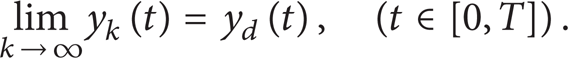
Given the desired output y _d (t) (t ∈ [0, T]), it is assumed that a unique desired output u _d (t) can be found. That is,

$\begin{array}{c}{y}_k^{\left(\alpha \right)}\left(t\right)=f\left(u_k,y_k,t\right),\\ y_d^{\left(\alpha \right)}\left(t\right)=f\left(u_d,y_d,t\right).\end{array}$

(4)

And the tracking error signal between the actual output y _k (t) and the desired one y _d (t) is

$e_k\left(t\right)=y_d\left(t\right)-y_k\left(t\right).$

(5)

3.2. The Convergence Condition

Based on the fractional order nonlinear system (1) and the fractional order ILC scheme (3), the following lemmas are introduced.

Lemma 1. For the fractional order nonlinear systems, suppose ${\parallel \partial f/\partial u\parallel }_{\infty }\le \gamma {\parallel u\parallel }_{\infty }$ ; then there exists a sufficiently large λ satisfying

${\parallel e_k\parallel }_{\lambda }\le O\left({\lambda }^{-\mathrm{1}}\right){\parallel \delta u_k\parallel }_{\lambda },$

(6)

where

$O\left({\lambda }^{-\mathrm{1}}\right)=\frac{\gamma \left(\mathrm{1}-e^{-\lambda T}\right)T^{\alpha }}{\lambda \Gamma \left(\alpha +\mathrm{1}\right)-c\left(\mathrm{1}-e^{-\lambda T}\right)T^{\alpha }}.$

(7)

It is important to introduce the λ-norm. The λ-norm for a function is defined as

${\parallel *\parallel }_{\lambda }=\underset{t\in \left[\mathrm{0},T\right]}{\sup }\left\{e^{-\lambda t}{\parallel *\parallel }_{\infty }\right\},$

(8)

where λ > 0 and ${\parallel *\parallel }_{\infty }={\max }_{t\in [\mathrm{0},T]}\{\left|*\right|\}$ denotes the maximum norm of the function.

Proof. This proof can be found in [23].

Lemma 2. For the fractional order nonlinear system (1) and the D^α-type ILC scheme (3), suppose δu _k (t) = u _d (t) − u _k (t), k = 0, 1, 2,…, and ${\parallel \partial f/\partial u\parallel }_{\infty }\le \gamma {\parallel u\parallel }_{\infty }$ ; then, one has

${\parallel \delta u_{k+\mathrm{1}}\parallel }_{\infty }\le \rho {\parallel \delta u_k\parallel }_{\infty },$

(9)

where ρ is defined in the following proof.

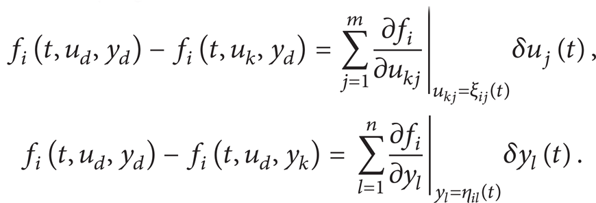
Proof. For the fractional order nonlinear system (1), it follows from (4) and (5) that

$\begin{array}{l}{f}_d-f_k\\ \hspace{1em}=f\left(t,u_d,y_d\right)-f\left(t,u_k,y_k\right)\\ \hspace{1em}=f\left(t,u_d,y_d\right)-f\left(t,u_d,y_k\right)+f\left(t,u_d,y_k\right)-f\left(t,u_k,y_k\right)\\ \hspace{1em}={\left\{\frac{\partial f_i}{\partial y_l}\right\}}_{{\eta }_{il}\left(t\right)}{e}_k\left(t\right)+{\left\{\frac{\partial f_i}{\partial u_{kj}}\right\}}_{{\xi }_{ij}\left(t\right)}\delta u_k\left(t\right)\\ \hspace{1em}=A\left(t\right)e_k\left(t\right)+B\left(t\right)\delta u_k\left(t\right),\end{array}$

(10)

where f is a continuous differentiable function, f _d = f(t, u _d , y _d ), f _k = f(t, u _k , y _k ), δu _k = u _d − u _k , and i, l ∈ {1, 2,…, n}, j ∈ {1, 2,…, m}. There exist functions ξ _ij (t) and η _il (t) satisfying

$\begin{array}{c}{f}_i\left(t,u_d,y_d\right)-f_i\left(t,u_k,y_d\right){={\displaystyle \sum }_{j=\mathrm{1}}^m\frac{\partial f_i}{\partial u_{kj}}‍|}_{u_{kj}={\xi }_{ij}\left(t\right)}\delta u_j\left(t\right),\\ f_i\left(t,u_d,y_d\right)-f_i\left(t,u_d,y_k\right)={{\displaystyle \sum }_{l=\mathrm{1}}^n‍\frac{\partial f_i}{\partial y_l}|}_{y_l={\eta }_{il}\left(t\right)}\delta y_l\left(t\right).\end{array}$

(11)

Then,

$\begin{array}{l}{\parallel \delta u_{k+\mathrm{1}}\parallel }_{\infty }={\parallel u_d-u_{k+\mathrm{1}}\parallel }_{\infty }\\ \hspace{1em}\hspace{1em}\hspace{1em}={\parallel \delta u_k-K_d{e}_k^{\left(\alpha \right)}\parallel }_{\infty }\\ \hspace{1em}\hspace{1em}\hspace{1em}={\parallel \delta u_k-K_d\left[f_d-f_k\right]\parallel }_{\infty }\\ \hspace{1em}\hspace{1em}\hspace{1em}={\parallel \delta u_k-K_d\left[A\left(t\right)e_k+B\left(t\right)\delta u_k\right]\parallel }_{\infty }\\ \hspace{1em}\hspace{1em}\hspace{1em}={\parallel \left[\mathrm{1}-K_{d}B\left(t\right)\right]\delta u_k-K_{d}A\left(t\right)e_k\parallel }_{\infty }\\ \hspace{1em}\hspace{1em}\hspace{1em}\le {\parallel \mathrm{1}-K_{d}B\left(t\right)\parallel }_{\infty }{\parallel \delta u_k\parallel }_{\infty }+{\parallel K_{d}A\left(t\right)\parallel }_{\infty }{\parallel e_k\parallel }_{\infty }.\end{array}$

(12)

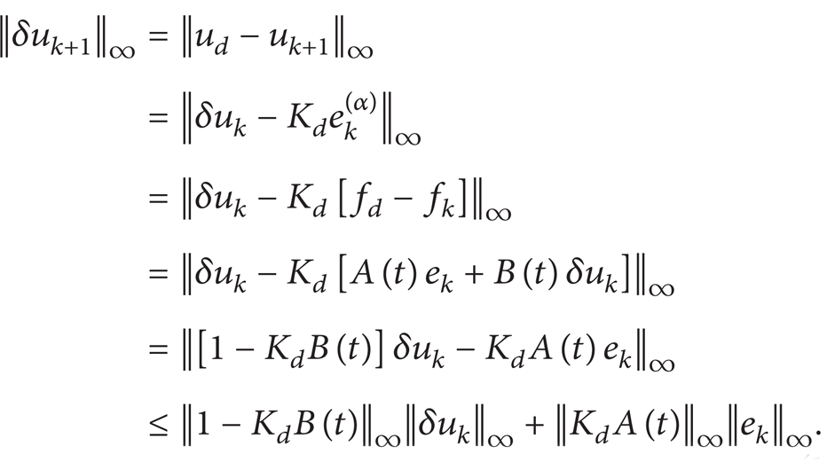
Applying the λ-norm to the above equation yields

$\begin{array}{l}{\parallel \delta u_{k+\mathrm{1}}\parallel }_{\lambda }\le \underset{\mathrm{0}\le t\le T}{\sup }{\parallel \delta u_{k+\mathrm{1}}\parallel }_{\infty }\\ \hspace{1em}\hspace{1em}\hspace{1em}\le \underset{\mathrm{0}\le t\le T}{\sup }\left\{{\parallel \mathrm{1}-K_{d}B\left(t\right)\parallel }_{\infty }{\parallel \delta u_k\parallel }_{\infty }\right\}\\ \hspace{1em}\hspace{1em}\hspace{1em}\hspace{1em}+\underset{\mathrm{0}\le t\le T}{\sup }\left\{{\parallel K_{d}A\left(t\right)\parallel }_{\infty }{\parallel e_k\parallel }_{\infty }\right\}\\ \hspace{1em}\hspace{1em}\hspace{1em}=\rho {\parallel \delta u_k\parallel }_{\lambda }+\omega {\parallel e_k\parallel }_{\lambda },\end{array}$

(13)

where

$\rho =\underset{\mathrm{0}\le t\le T}{\sup }{\parallel \mathrm{1}-K_{d}B\left(t\right)\parallel }_{\infty },\hspace{1em}\hspace{1em}\omega =\underset{\mathrm{0}\le t\le T}{\sup }{\parallel K_{d}A\left(t\right)\parallel }_{\infty }.$

(14)

Using Lemma 1 and (13) yields

${\parallel \delta u_{k+\mathrm{1}}\parallel }_{\lambda }\le \left(\rho +\omega O\left({\lambda }^{-\mathrm{1}}\right)\right){\parallel \delta u_k\parallel }_{\lambda },$

(15)

so let λ → ∞, ${\parallel \delta u_{k+\mathrm{1}}\parallel }_{\infty }\le \rho {\parallel \delta u_k\parallel }_{\infty }$ .

Theorem 3. For the fractional order nonlinear system (1) with the D^α-type ILC scheme (3), where t ∈ [0, T], suppose f(t, u, y) satisfies (2), and there exists a learning gain K _d satisfying

${\parallel \mathrm{1}-K_d\frac{\partial f}{\partial u}\parallel }_{\infty }<\mathrm{1},$

(16)

and then one has

$\underset{k\to \infty }{\lim }{y}_k\left(t\right)=y_d\left(t\right),\hspace{1em}\left(t\in \left[\mathrm{0},T\right]\right).$

(17)

Proof. It follows from Lemma 2 and (2) that ${\parallel \delta u_{k+\mathrm{1}}\parallel }_{\lambda }\le [\rho +\omega O({\lambda }^{-\mathrm{1}})]{\parallel \delta u_k\parallel }_{\lambda }$ . Using (16) yields ρ < 1, so that there is a sufficiently large $\tilde{\lambda }$ satisfying $\rho +\omega O({\tilde{\lambda }}^{-\mathrm{1}})<\mathrm{1}$ . Therefore,

$\underset{k\to \infty }{\lim }{\parallel \delta u_k\parallel }_{\tilde{\lambda }}=\underset{k\to \infty }{\lim }{\parallel u_d-u_k\parallel }_{\tilde{\lambda }}=\mathrm{0}.$

(18)

In other words, lim⁡_{k → ∞}u _k (t) = u _d (t), where t ∈ [0, T]. It then follows from the uniqueness and existence theorem for fractional order differential equations [21] that lim⁡_{k → ∞}y _k (t) = y _d (t).

Remark 4. It can be seen from Theorem 3 that the key points of the learning law (3) in convergence analysis are the learning gain K _d and the learning order α. The learning gain K _d depends on the approximation of B(t), where a small enough K _d can surely guarantee the convergence but sacrifices the convergence speed, and the optimal K _d can be derived from the identification of B(t), which is a tremendous hard work in reality. On the other hand, the global Lipschitz condition provides a reliable way to linearize the nonlinear system (1) by using Taylor's expansion. Thus, the optimal learning order α points to the fastest convergence speed [24], which can be easily verified in simulations or experiments by using the fractional order ILC schemes.

Therefore, allow for the applications and the implementations of the D^α-type ILC scheme, and the ILC scheme in (3) is replaced by

$U_{k+\mathrm{1}}\left(s\right)=U_k\left(s\right)+K_d\left(s\right)E_k\left(s\right),$

(19)

where K _d (s) plays a role as a differentiator plus a low-pass filter so that this scheme can be called fractional order D^α-type low-pass ILC.

A very large group of filters can be applied to the above algorithm. Here, we unify the filter in frequency domain in the form of

$K_d\left(s\right)=\frac{kp{s}^{\alpha }}{\left(\mathrm{1}+\beta s^{\text{alpha}}\right)},$

(20)

${\alpha }_{l+\mathrm{1}}={\alpha }_l+TE\left(e_l\right),\hspace{1em}T>\mathrm{0},$

(21)

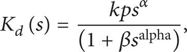
where kp and β are positive constants. The value of β is very small such that (20) plays like a fractional order operator cascaded after a fractional order low-pass filter. The α in (20) is the order of ILC updating law, which is an arbitrary real number less than or equal to the order of the dimensional error compensation system. In fact, it has been proved and verified in fractional order linear cases that the convergent speed is the fastest when the system and iterative learning scheme have the same order [24]. The relation of α and alpha satisfies 0 < α ≤ alpha < 1. The order updating law is shown in (21), and E(e _l ) is the average error of the l_th iterative learning cycle.

3.3. Compensation Method

As previously discussed, there are many factors resulting in the dimensional errors, which are presented nonlinearly and nonmonotonously. In order to overcome the nonlinear characteristic of dimensional errors and keep the machined dimensions within the tolerance over successive cycles, the following compensation procedures are implemented.

1. The compensation direction is defined as follows:

   $E\left(k\right)=\text{Dime}-D\left(k\right)$

   (22)

   if (E(k) > E _lim ),

   then Sc(k) = − 1;

   else if (E(k) < − E _lim ),

   then Sc(k) = 1;

   else Sc(k) = 0.

   Here Dime is the desired dimension of workpieces and D(k) is the dimension of the k_th workpiece. Sc(k) is a compensation mark indicating whether error compensation will be executed or not and in which direction the compensation will be. If Sc(k) = 0, the dimensional error E(k) of a processed workpiece is within the acceptable error limit E _lim , and the error compensation is bypassed. When Sc(k) = − 1, negative compensation will be applied; otherwise, the compensation will be positive. Note that the value of acceptable error limit E _lim affects oscillation of the compensating system output; a larger value of E _lim tends to better damp oscillation, although at the expense of dimensional variation.

2. The amount of compensation C(k + 1) to be implemented before the ${(k+\mathrm{1})}_{\text{th}}$ workpiece to be machined is computed as

   $C\left(k+\mathrm{1}\right)=C\left(k\right)+\Gamma \left(k\right)*E\left(k\right).$

   (23)

   Here, the filter in (20) and the updating law of α in (21) are introduced to compute C(k + 1). The filter in (20) needs to be transformed into discretion form and then switches to time domain. With this method, unrepeatable signals, such as noise, located in high frequency, will be decayed.

3. To avoid excessive fluctuation of the workpiece dimension caused by measurement noise and other uncontrollable factors and to ensure the safety of the machine tool, the compensation limit (C_max) is introduced on the computed compensation C_{k + 1}. This is implemented as follows:

   if (Sc(k) ==1&C(k + 1) > C_max),

   then C(k + 1) = C_max;

   else if (Sc(k) = = − 1&C(k + 1) < − C_max),

   then C(k + 1) = − C_max.

4. Learning Law Optimization and Experimental Verification

Since the compensation procedures have been determined, the next step is to optimize the ILC updating law and to verify the efficiency of the proposed dimensional error precompensation scheme in CNC batch grinding. The optimization process is to identify the order of the ILC updating law, which is also the order of the system.

For learning law optimization and verification, the major assumption is that since the X axis distance between the grinding wheel and the C axis is kept constant while recording the baseline data, any incremental change made to this distance in the simulation is to be reflected in the resulting relative workpiece dimension.

The baseline dimensions of workpieces shown in column 2 of Table 1 are used to identify the system order and verify the compensation strategy. The experiment is conducted on a 3-axis machine tool: 2MBK7125. The model for such batch workpieces is SPCN1504EDR, and the material is YT15. The grinding conditions for this batch are shown in Table 2.

Table 1:

Dimensional comparison of the machined workpiece before and after compensation.

Number	Dimensions of the group of machined workpieces without compensation (mm)	Error compensation simulation result of the group workpieces (mm)
1	15.844	15.844
2	15.845	15.865
3	15.847	15.859
4	15.845	15.857
5	15.848	15.86
6	15.847	15.859
7	15.847	15.859
8	15.852	15.864
9	15.857	15.863
10	15.856	15.862
11	15.85	15.856
12	15.853	15.865
13	15.853	15.857
14	15.857	15.861
15	15.854	15.858
16	15.857	15.861
17	15.86	15.864
18	15.858	15.856
19	15.859	15.863
20	15.865	15.864
21	15.864	15.857
22	15.865	15.863
23	15.863	15.861
24	15.873	15.871
25	15.87	15.851
Numbers of workpieces within the dimensional tolerance 0.005 mm	11	22
Average error	−0.00444	0.000042254

Table 2:

Grinding conditions for workpieces.

Parameters	Value
Diamond wheel	Resin bonded, mesh# 220, concentration 100%
Wheel diameter (mm)	350
Wheel rotation (mm/s)	18
Feed rate (mm/s)	0.03∼0.05
No spark time (s)	2
Coolant	Water soluble

For optimization and verification, the parameter values are defined as follows: t = 0.00001, E _lim = 0.003, and C_max = 0.02. Since t is a small positive constant, the value of it is defined as 0.00001. As previously mentioned, the value of E _lim affects the oscillation of the compensating system output; a larger value of E _lim tends to better damp oscillation, although it is at the expense of dimensional variation. Since the accepted error tolerance of A level workpiece is ± 0.005 mm, in order to decrease dimensional variation, the value of error limit E _lim is chosen as 0.003. Amplitude limit C_max is obtained by historical data, in order to achieve high precision and operate safely, and the value is defined as 0.02.

The identification of the order is conducted in the following 3 steps.

Step 1. For (20), the initial value of alpha is 1, and the initial value of α is 0. Take simulation for the baseline data and record the average error of this iterative learning cycle.

Step 2. Keep the value of alpha the same as in Step 1 and update α as in (21). Take simulations until E(e _n ) ≤ ɛ; ɛ is a very small positive constant. Record parameters of the iterative learning cycle with minimum average error.

Step 3. The parameter alpha is updated in the following way:

${\text{alpha}}_{m+\mathrm{1}}={\text{alpha}}_m-\mathrm{0.05}.$

(24)

Switch to Step 2 and take simulations until the end. Note that the updating law of alpha is important to the convergence rate of ILC scheme as well as the complexity of estimation. Here, an incremental order updating law in (24) is defined for alpha. This form is easy to implement, meanwhile guaranteeing the convergence rate. Combined with (20) and (21), the system order can be estimated. Besides, the parameter kp is a positive constant, whose value is determined by the convergence condition.

The results of identification are shown in Table 3. From it, we can see that there is not an optimal value for the order of the ILC updating law and the system. Because of the time-variant characteristic of the system, the order is in 0.6∼0.64. With the group of parameters, α = 0.64, alpha = 0.95, and kp = 12, the dimensions after using the fractional order iterative learning compensation scheme are shown in column 3 of Table 1.

Table 3:

The identification results.

α	Average error	Variance	Numbers of level workpieces
0.58	0.00033976	0.000029628	21
0.59	0.00027721	0.000030245	21
0.6	0.00022724	0.000025410	22
0.61	0.00017521	0.000025646	22
0.62	0.00012672	0.000025873	22
0.63	0.000081884	0.000026089	22
0.64	0.000042254	0.000026285	22
0.65	0.000052122	0.000029515	18
0.66	0.000084051	0.000029793	18
0.67	0.00011006	0.000030021	18
0.68	0.00012809	0.000030179	18
0.69	0.00013762	0.000030263	18
0.70	0.00013776	0.000030264	18

Beyond the scope of the system order, the dimensions present divergence. Note that workpieces whose dimensional error within the error tolerance [−0.005, 0.005] are A level. Figure 5 shows the comparison of dimensional variation before and after error compensation. For the group of workpieces, the desired dimension is 15.860 mm. From Table 1 and Figure 5, it is evident that there are only 11 workpieces out of 25 within the error tolerance [−0.005, 0.005] before error compensation, while after error compensation, the amount increases to 22. The average error of this batch decreases from −0.00444 to 0.000042254, and the variance decreases from 0.000062166 to 0.000026285. In our earlier studies [12], the PD-type ILC compensation scheme was applied to the CNC grinding process. For the same batch workpieces, the average error computed in [12] is 0.00037308 and the variance is 0.000019879. Comparing the fractional order D^α-type ILC scheme with the integer order PD type ILC, it is clear that the average error is much smaller using fractional order iterative learning compensation scheme.

Figure 5:

Dimensional variation of the group chips before and after fractional order iterative learning error compensation.

Remark 5. The globally Lipschitz condition guarantees the linear discretization of the nonlinear system (1), so that it follows from [24] that the optimal FOILC is pointing to the D^α one, where α is exactly the same as the system order α. Therefore it can be seen from Table 3 that, given the nonlinear structure of the CNC grinding system (1), the system order can be estimated by using (20) and (21) as well as the incremental order updating law (24) without any knowledge of system parameters.

5. Conclusions

This paper proposes an intelligent dimensional error compensation method using fractional order iterative learning strategy. Compared with previous methods [3–11], this approach has the following advantages: (1) there is no need for other sensors to detect the geometric, thermal, and cutting force-induced errors, nor is a mathematical model necessary for predicting the dimensional error; (2) the dimensional measurement and error compensation are executed in every machining cycle, only a touch probe to be used for part dimension measurement, which makes this technique easy to be implemented; and (3) it is suitable for any type of multiaxis machine tools.

This paper also introduces the fractional order ILC theory into precision control. The identification and simulation results clearly show that the dimensional error precompensation system is a fractional order system, and the order is about 0.6∼0.64. The response of the precompensation scheme guarantees the effectiveness of this dimensional accuracy enhancement technique. With this intelligent scheme, the machined workpiece dimension will remain within its tolerance over successive machining cycles.

Conflict of Interests

The authors declare that there is no conflict of interests regarding the publication of this paper.