A Hybrid Node Scheduling Approach Based on Energy Efficient Chain Routing for WSN

Abstract

Energy efficiency is usually a significant goal in wireless sensor networks (WSNs). In this work, an energy efficient chain (EEC) data routing approach is first presented. The coverage and connectivity of WSNs are discussed based on EEC. A hybrid node scheduling approach is then proposed. It includes sleep scheduling for cyclically monitoring regions of interest in time-driven modes and wakeup scheduling for tracking emergency events in event-driven modes. A failure rate is introduced to the sleep scheduling to improve the reliability of the system. A wakeup sensor threshold and a sleep time threshold are introduced in the wakeup scheduling to reduce the consumption of energy to the possible extent. The results of the simulation show that the proposed algorithm can extend the effective lifetime of the network to twice that of PEAS. In addition, the proposed methods are computing efficient because they are very simple to implement.

1. Introduction

Since the nodes in WSN are battery-powered, energy conservation is always a focus of research. The main roles for nodes are detecting the state of the environment and sending data packets. Many measurements have been taken showing that idle listening consumes 50–100% of the energy required for receiving [1]. Hence, the most efficient method is to turn off the radio when there is no need to transmit or relay packets. Sensor scheduling aims to maintain a balance of network resources [2]. Many sleep and wakeup scheduling strategies have been proposed to save energy in recent years. There are two categories of node scheduling methods.

The first category is sleep-wake scheduling, in which all nodes are put to sleep and some nodes woken up according to wakeup strategies. Sleep-wake scheduling strategies can be divided into two main categories: scheduled wakeup and wakeup on demand [3]. Scheduled wakeup mechanisms include synchronous and asynchronous wakeup mechanisms. The scheduled wakeup mechanisms might miss the occurrence of an important event when the nodes are in sleep mode, such as the detection of an intrusion. Synchronization procedures could lead to the incurring of additional communication overhead and consume a considerable amount of energy [4]. On-demand wakeup mechanisms have to wait for the next-hop node to be woken up.

The second category of node scheduling method is sleep scheduling, in which redundant idle nodes are turned off according to duty-cycle mechanisms, so as to extend the lifetime of the network and keep the stem nodes awake to detect events and deliver data. Most of these algorithms define several states of operation for the nodes and provide different state-transition strategies according to the requirements. Examples include some famous algorithms: ASCENT [5], GAF [6], and PEAS [7]. New approaches are constantly being proposed. VBS [8] provides a mechanism to schedule multiple backbones to work alternatively. A. Mutazono et al. proposed a strategy of self-organizing sleep schedules based on tree-frog satellite behavior in [9]. Wang et al. discussed the network from the perspective of computational geometry in [10]. The scheduling algorithm achieved high coverage by very few nodes and minimized the network's energy consumption. GSSC conserves energy by finding equivalent nodes from a routing perspective by using their geographical information (i.e., the nodes that sense almost the same information) and then turning off unnecessary nodes to remove redundant data [11].

Network coverage and connectivity are fairly important issues in work such as the above. To build connections, all sleep-wake scheduling strategies in the first category suffer from delays, which is unacceptable for delay-sensitive applications. Researchers have to solve such delay problems [4, 12–16] to guarantee the connectivity of the network while reducing energy consumption. In the second category, most node scheduling algorithms have some strategies to guarantee the coverage and connectivity of the networks. ASCENT is based on stable coverage and connectivity. Backbone nodes in VBS are defined to preserve network connectivity. GAF and PEAS guarantee network coverage and connectivity based on a grid partition. The grid partition in GAF should be small enough to ensure coverage. GSSC guarantees network coverage and connectivity by waking the equivalent nodes up. On the other hand, cover scheduling for WSNs has attracted a great deal of attention. As full coverage is extremely expensive, cover scheduling is employed to schedule the covers so as to minimize the longest period of time during which a target is not covered in the schedule [17].

However, these approaches assume that the nodes work at the same working mode, whether event-driven or time-driven, during their whole lifetime. In this paper, we are concerned about such real applications in which the nodes work in both a time-driven mode to periodically detect situations in the environment and in an event-driven mode to trace emergency events at once. A hybrid node scheduling algorithm based on partition is proposed for these applications. The main contributions of this paper are as follows. (1) An energy efficient chain routine is proposed for large-scale WSNs, which is the foundation of the scheduling approaches in this paper. (2) The conditions of a schedulable node set that can guarantee network connectivity and coverage are defined. (3) A reliable sleep scheduling approach is proposed to keep one node work reliably in each grid and turn off redundant nodes to reduce energy consumption in time-driven working modes. (4) A wakeup scheduling approach is proposed to wake more nodes up to guarantee the maximum coverage, in order to precisely trace the trend of an emergency event in event-driven modes.

The rest of this paper is organized as follows. The system model is described in Section 2. The energy efficient chain data routing approach, which is based on tier division according to a radio energy consumption model, is presented in Section 3. In Section 4 the coverage and connectivity based on grid partition are discussed, and the condition of a schedulable node set is presented. The sleep scheduling and wakeup scheduling are introduced in detail in Section 5. The simulation results and analysis are given in Section 6. Conclusions are presented in Section 7.

2. System Model

2.1. Network Model

In our work, the sensor nodes in WSNs are relatively evenly distributed around a unique base station (BS). The BS is located very far away from the sensor field, as shown in Figure 1.

Figure 1:

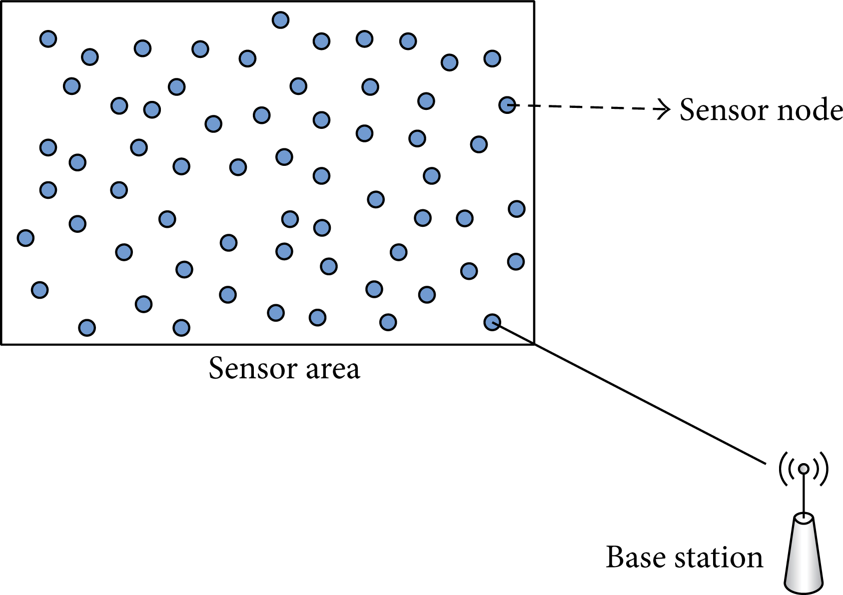
BS and the distribution of nodes in WSN.

The nodes are sufficient to cover the whole region, and there are many redundant nodes. Suppose the number of sensor nodes in the network is n. We use the following assumptions in our WSN model.

• All of the nodes and the BS are stationary after deployment.

• The position of each node is known.

• Every node can access the BS. However, the nodes will run out of energy very soon if they transmit message to BS directly.

• Each node has a unique identifier (ID).

• All of the sensor nodes are homogeneous and power is limited. All of the nodes have the same initial energy E₀, the same broadcasting radius R _b , and the same probing radius R _p ; the same furthest transmitting radius of all of the nodes is R _t . R _b , R _p , and R _t are fixed for nodes whose value is decided by the hardware of the sensors.

• Sensor nodes are capable of changing their transmitting power. That means that the transmitting radius R _t (i) is changeable for node i.

• Individual nodes may fail unexpectedly so that the coverage and connectivity may not be maintained.

2.2. Application Scenarios and Working Modes

In this paper, we are concerned with relatively evenly deployed large-scale WSNs as are applied to monitor situations in a region of interest. The application scenarios and the working modes are shown in Figure 2.

Figure 2:

The application scenarios and the working modes.

In most cases, the nodes periodically collect information of interest about the region, which is called the time-driven working mode. In time-driven working mode, our main goal is to reduce the power consumption. When a special event occurs, such as a forest fire, gas leakage, military intrusion, and the tracking of endangered animals, the nodes need to track the trend of the event with timeliness and precision. This is called the event-driven working mode. In event-driven working mode, the highest priority task is to trace the event trends and taking account of the reduction of the power consumption.

There are many redundant nodes in these randomly deployed large-scale WSNs to fulfill the above tasks. To save energy, some redundant nodes can be put in sleep and they can be woken up at any point of time if necessary, as assumed in [18–20].

3. Energy Efficient Chain Data Routing

In energy efficient chain data routing, we divided the node into tiers according to the radio energy dissipation model (REDM) [21]. Nodes then send data to the nearest node in the next tier, which is nearer to BS.

3.1. Principle of Tier Division

REDM shows that the energy dissipation is related to the transmitting distance between two nodes. According to REDM, the energy consumed in transmitting k bit messages is given as

$\begin{array}{l}{E}_{\text{Tx}}\left(k,d\right)=E_{\text{Tx-elec}}\left(k\right)+E_{\text{Tx-amp}}\left(k,d\right)\\ \hspace{1em}\hspace{1em}\hspace{0.17em}=\{\begin{array}{cc}k{E}_{\text{elec}}+k{\epsilon }_{\text{fs}}\times d^{\mathrm{2}},\hfill & d\le d_{\mathrm{0}}\hfill \\ k{E}_{\text{elec}}+k{\epsilon }_{\text{mp}}\times d^{\mathrm{4}},\hfill & d>d_{\mathrm{0}}.\hfill \end{array}\end{array}$

(1)

The energy consumed in receiving this message is

$E_{\text{Rx}}\left(k\right)=E_{\text{Rx-elec}}\left(k\right)=k{E}_{\text{elec}}.$

(2)

Formula (3) is used to calculate the receiving power P_rx [22]:

$P_{\text{rx}}\left(d\right)=P_{\text{tx}}\times \left(\frac{\epsilon }{d_{\text{to}\hspace{0.17em}\text{BS}}^{\mathrm{4}}}\right).$

(3)

In (3), P_tx is the BS transmitting power; ε is the attenuation factor; and the value of ε is related to the emission gain, the receiving antenna, the system loss parameter, and the wavelength. Usually, P_tx is a constant, so the distance between nodes and the BS can be calculated by

$d_{\text{to}\hspace{0.17em}\text{BS}}=\frac{r}{\sqrt[\mathrm{4}]{P_{\text{rx}}}}.$

(4)

In (4), r is a constant. Assuming that D is the radius of the tier, if d_{to BS}(i) satisfies l × D ≤ d_{to BS}(i) < (l + 1) × D, then the tier ID of N(i) is l.

3.2. Selection of the Ring Radius of Each Tier

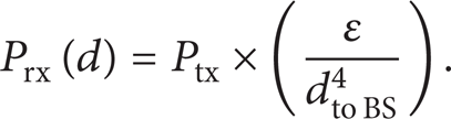
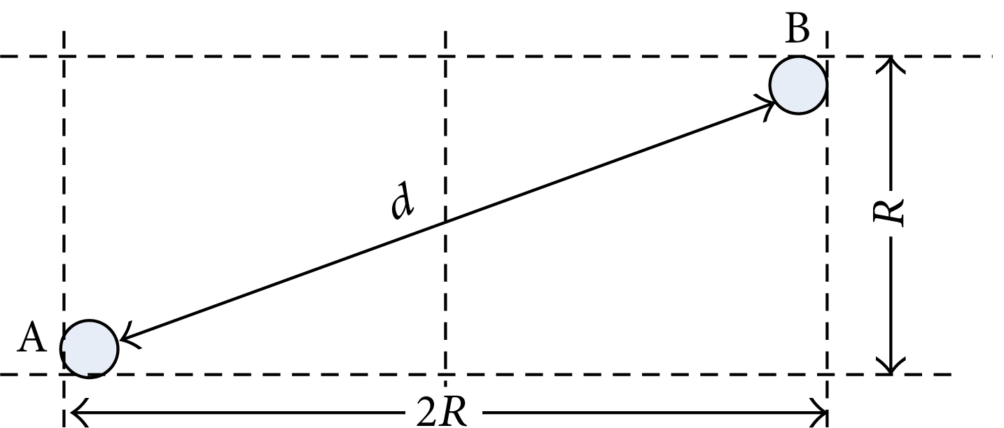
The value of D is determined by d₀. According to (1), the energy consumption is proportional to d² if d ≤ d₀, while the energy consumption is proportional to d⁴ if d > d₀. To save energy, EEC requires the transmitting distances both between two tiers and between two nodes in a tier to be less than d₀. That means the transmitting distance between two neighbor tiers must be less than d₀. In the worst case, as shown in Figure 3, to guarantee that the distance between node A and node B is less than d₀, the ring radius of each tier should be approximately less than $d_0/\sqrt{5}$ . In practice, because the sensor field is far away from the BS, the arc line can be considered an approximate line.

Figure 3:

Ring radius of each tier in the worst case.

3.3. Deciding the Tier of Each Node

Set $D=d_0/\sqrt{5}$ , if d_{to BS}(i) satisfies

$l\times \frac{d_0}{\sqrt{5}}\le d_{\text{to}\hspace{0.17em}\text{BS}}\left(i\right)<\left(l+\mathrm{1}\right)\times \frac{d_0}{\sqrt{5}}.$

(5)

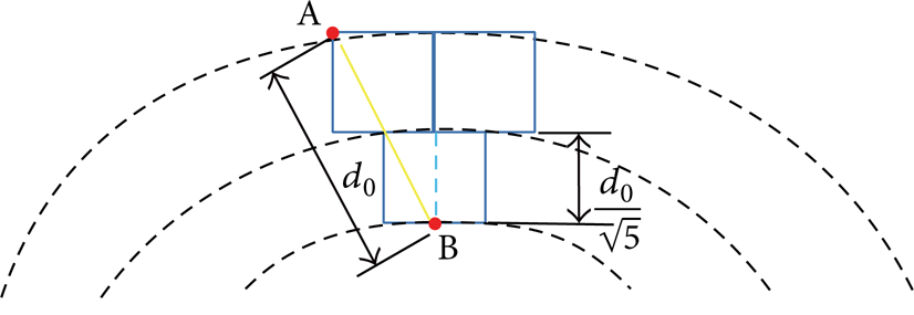
Then the tier of N(i) is l. Figure 4 shows the tier division of the network. The network is divided into four tiers, and tier ID is L _i , where i = 1, 2, 3, 4, and L _i = i.

Figure 4:

The tier division of nodes in WSN.

3.4. Building Chain Routine

Each sensor node directly transmits the data to the nearest node in the next lower tier. Because the BS is located far from the sensor area, the radian of each tier can be omitted. The final routine is a node-to-node path. A node with a higher tier ID sends data to its nearest neighbor with a lower tier ID. The data is transmitted tier by tier and finally forwarded to the node in the top tier, which is responsible for eventually forwarding the data to the BS. Supposing that there are m tiers in the network, the routing will be L _m →L_{m − 1}→⋯→L₂→L₁→ BS. The network routing is shown in Figure 5.

Figure 5:

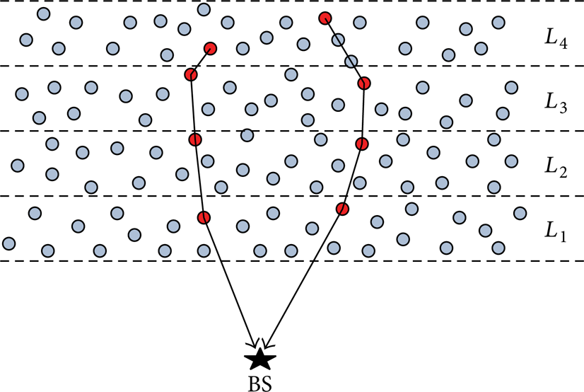
Examples of the proposed chain routing for WSN.

4. Coverage and Connectivity

Because there are many redundant nodes, these redundant nodes can be put to sleep to save energy. However, a useful sleep scheduling approach should extend the effective working time of the network. That means that the node scheduling strategy should maintain the coverage and connectivity of the network. However, full coverage is our expectation. The following is our definition of the effective working time of a network.

Definition 1. The effective working time of a network is the lifetime of the network, which satisfies the following conditions.

1. The nodes can cover the whole area of interest.

2. The states of each monitoring region can be transmitted to the BS.

The coverage and connectivity required to guarantee that the WSN works effectively will be discussed in the following sections.

4.1. Coverage of the Network

The node scheduling mechanism is only applied to those nodes with coverage overlap. But it is difficult to identify and manage coverage overlap in a whole network. Therefore, we partition the whole monitoring area into equal grids with the size of R × R, as shown in Figure 6.

Figure 6:

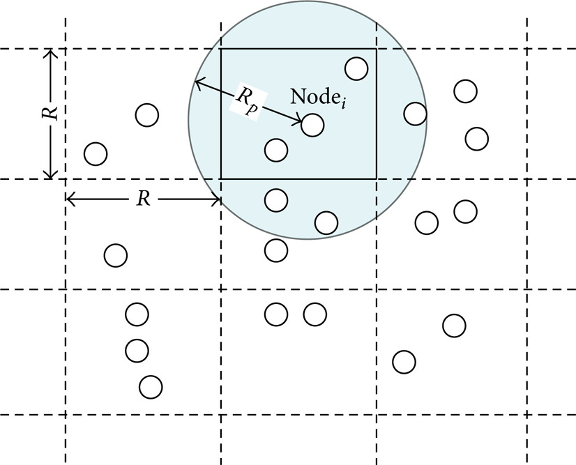
Grid partition of the network.

Assume that every partition has a unique ID. In the beginning, every node can get its own position by some location method, such as GPS. The coverage overlap of nodes in a grid is known. It is then possible to manage the coverage redundancy in each grid. If the coverage overlap of nodes in different grids is ignored, the coverage redundancy in each grid is easily identified and managed.

In this paper, we focus on the node coverage in each grid, which depends on the node position and R _p . The division of the grids will change correspondingly as R changes. The position is different for the same node in a grid with a different R. As shown in Figure 7, in the best case, the node locates at the center of a grid and it will completely cover the grid if $R\le \sqrt{\mathrm{2}}{R}_p$ . In the worst case, the node locates at a vertex of the grid and it will completely cover the grid if $R\le \sqrt{\mathrm{2}}/\mathrm{2}{R}_p$ .

Figure 7:

Values of R in the best case and the worst case.

If $R\le \sqrt{\mathrm{2}}/\mathrm{2}{R}_p$ , a grid can be completely covered by each node located anywhere in the grid. However, there will be serious overlapping even if only one node is working in each grid when R satisfies $R\le \sqrt{\mathrm{2}}/\mathrm{2}{R}_p$ . The best solution for this overlap is to choose a suitable value for R so that the probing area inside the grid is largest and the probing area outside the grid is smallest for all nodes in random positions in the grid. Obviously, the greater the R is, the larger the probing area inside the grid will be. But, in that case, there will be larger coverage holes. Hence, the range of R should satisfy the following conditions:

$\frac{\sqrt{\mathrm{2}}}{\mathrm{2}}{R}_p\le R\le \sqrt{\mathrm{2}}{R}_p.$

(6)

If complete coverage is not necessary, then $R=\sqrt{\mathrm{2}}{R}_p$ is an acceptable choice. However, when $R=\sqrt{\mathrm{2}}{R}_p$ and the coverage of nodes in other grids is ignored, there will be some coverage holes in a grid if the node does not locate at the center of the grid. However, the nodes in other grids might cover most of the area of this coverage hole because the nodes are randomly distributed and there are always coverage areas outside a node's own grid.

4.2. Connectivity of the Network

The entire wireless sensor network can be regarded as an undirected-graph. If a node called the cut point of the undirected-graph is turned off, the network connectivity will be broken, as shown in Figure 8. To keep the connectivity, all cut points must keep on working. We can find all cut points in the network using the algorithm proposed in [23].

Figure 8:

Cut point in an undirected-graph.

First, the following definitions are given.

Definition 2. If node j in tier L _k is directly connected to node i in tier L_{k − 1}, node j is called the neighbor node of node i and node i is called the neighbor node of node j as well.

Definition 3. If node j has no neighbor node in the network, it is an isolated node.

Due to Definition 3, if the distance between a node and its nearest neighbor node is further than R _t , the node is an isolated node. To keep the network connectivity, the node scheduling approach should avoid creating such an isolated node.

In addition, to guarantee that there is at least one working node in each tier, R should satisfy the following equation:

$\frac{d_{\mathrm{0}}}{\sqrt{\mathrm{5}}R}=k,$

(7)

where k is a positive integer.

In the extreme case, the working nodes locate at the two furthest opposite vertexes A and B of adjacent grids, as shown in Figure 9. When node A is the nearest neighbor node of node B, these two nodes can communicate to each other only if the distance d between them is shorter than R _t . Since d satisfies the following equation:

$d^{\mathrm{2}}=R^{\mathrm{2}}+\mathrm{4}{R}^{\mathrm{2}},$

(8)

R should satisfy

$R\le \frac{\sqrt{\mathrm{5}}}{\mathrm{5}}{R}_t.$

(9)

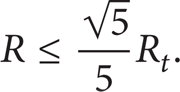
Generally, the transmitting radius is very much farther than the probing radius; that is, R _t ≫ R _p . Assume $R_t>\sqrt{\mathrm{10}}/\mathrm{2}{R}_p$ . Combined with the conditions in (6), the range of R should be

$\begin{array}{c}R\in \left[\frac{\sqrt{\mathrm{2}}}{\mathrm{2}}{R}_p,\frac{\sqrt{\mathrm{5}}}{\mathrm{5}}{R}_t\right],\hspace{1em}{R}_t\le \sqrt{\mathrm{10}}{R}_p\\ R\in \left[\frac{\sqrt{\mathrm{2}}}{\mathrm{2}}{R}_p,\sqrt{\mathrm{2}}{R}_p\right],\hspace{1em}{R}_t\ge \sqrt{\mathrm{10}}{R}_p.\end{array}$

(10)

Meanwhile, (8) should be satisfied.

Figure 9:

The extreme case of the location of nodes.

4.3. Schedulable Node Set

We only focus on those nodes that can be turned off without negative effects on network coverage and routing connectivity. A schedulable node set is defined as follows.

Definition 4. A node is a schedulable node in A _j , 0 < j ≤ M, where M is the total number of the grids in the whole network, if the node in grid A _j meets all of the following conditions.

1. The node is not a cut point.

2. The node is not an isolated node.

3. The node is not a unique node in A _j .

All schedulable nodes in A _j construct the schedulable node set S _j of grid A _j , 0 < j ≤ M.

In this paper, only the nodes in a schedulable node set can be put to sleep. The schedulable nodes in each grid are scheduled independently. Since there are more and more dead nodes with depleted energy in the network, the connectivity will change. Therefore, the scale of the schedulable node set is being continuously reduced. In the following sections, “node” always refers to a schedulable node.

5. Hybrid Node Scheduling

Node scheduling is a scheme of compromise, involving assigning as few nodes as possible to work, in order to save energy, while promising that the network will achieve its work goals. Generally, most of the time, the network is working in a time-driven mode to periodically collect information about the environment. If there is a working node in each grid, the network can monitor all of the grids. Therefore, if it can be guaranteed that there will always be a working node in each grid, we can turn off redundant nodes in the grid to reduce the consumption of energy. However, some significant events might occur between two intervals of acquisition. It is necessary to awaken more nodes to track unusual events in the region of surveillance if such events are emerging and a close watch needs to be kept on them. Moreover, more nodes should be woken up because some coverage holes might exist.

The proposed algorithm includes two scheduling methods: (1) a cyclical node sleep scheduling mechanism that cyclically assigns only one node to work in each grid and turns off other nodes and (2) an event-driven node wakeup mechanism that wakes more nodes up to track significant event trends. In the proposed algorithm, each node has four states: initializing, working, sleeping, and assisting. Suppose that in the beginning all nodes are in a sleeping state. Each node enters the initializing state to start the network after a period that is preset in the node. The scheduling mechanism will be described in detail below.

5.1. Cyclical Node Sleep Scheduling

Cyclical node sleep scheduling includes two parts: an initialization mechanism and a sleep scheduling mechanism.

5.1.1. The Initialization Mechanism

All nodes are initially in the sleeping state. After a preset time t₀, all nodes enter the initializing state and all nodes can receive messages from other nodes. In the initializing state, nodes in the grid A _j begin to send a probing message to each other, 0 < j ≤ M. t_start(i) is the time that the ith node in grid A _j begins to send the probing message. To avoid colliding, t_start(i) gets a random value in [0, T_init], with T_init being the allowable initializing time.

During the initializing time, each node explores whether there is a working node in A _j by sending a probing message. If a node did not receive a message about a working node claim in the grid, the node will enter the working state and set itself as the first working node in the node queue. The node queue is shown in Figure 10. The node will work in turn according to the ring queue starting from node 1.

Figure 10:

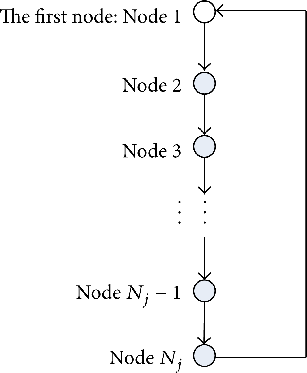
Node queue in grid A _j .

The exploring procedure is described as in Algorithm 1.

Algorithm 1:

The node exploring procedure in A _j .

The node with the minimum t_start(i) in A _j generally elects to be the first working node. Because it is the first one to send a message, it did not receive any messages, including a working node claim, when t = min⁡{t_start(i)}, as shown in Figure 11. If there is one working node, the other nodes communicate with the working node to build the node queue and then go back to the sleeping state. The working node builds the node queue according to the sequence of nodes applying to join the node queue. The information on the node queue is stored in the first working node and will be sent to the next working node when the node is woken up to work. Because t_start(i) is different for I = 1, 2,…, N _j , the node queue in grid A _j is sorted by t_start(i) in an ascending fashion.

Figure 11:

Exploring during the initialization time.

5.1.2. Sleep Scheduling

In a time-driven mode, there should be only one node in a working state in each grid at any time. In order to extend the lifetime of a network, the nodes in a grid should work in turn. The simplest scheduling is for the working node to wake the next node up in the node queue, one after one. But this may lead to some areas that have not been monitored for a long time because some coverage holes exist. In the proposed algorithm, each node will transit in state in accordance with a scheduling cycle to avoid having some areas that cannot be monitored for a very long time. In addition, a node may unexpectedly fail because its failure rate is not zero.

A node should not be switched to the sleeping state when it is collecting data. To ensure that this is the case, the time spent by the node in the working state should be longer than the time spent in collecting data. Assuming that the data acquisition cycle is T_collect, which is usually determined by demand, the time spent in collecting data is t_collect, the idle time during each T_collect is t_idle, the scheduling cycle is T_schedule(j) in grid A _j , and the communication time is negligible. In a scheduling cycle of A _j , t_work(j) is the working time, t_sleep(j) is the sleeping time, and there is

$\begin{array}{c}{T}_{\text{collect}}=t_{\text{collect}}+t_{\text{idle}},\\ T_{\text{schedule}}\left(j\right)=t_{\text{work}}\left(j\right)+t_{\text{sleep}}\left(j\right).\end{array}$

(11)

To guarantee that the WSN works well, there must be

$t_{\text{work}}\left(j\right)\ge t_{\text{collect}}.$

(12)

5.1.3. Reliable Sleep Scheduling Based on the Failure Rate

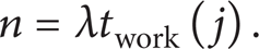
To improve the reliability of the system, the notion of the node failure rate was introduced. Assume that the node failure rate is a constant λ. Since each node in grid A _j works continuously for period of t_work(j) in a scheduling cycle, the number of failures n for a node satisfies

$n=\lambda t_{\text{work}}\left(j\right).$

(13)

To ensure that the node does not fail during its working time, n should satisfy

$n<\mathrm{1}.$

(14)

This means that

$t_{\text{work}}\left(j\right)<\frac{\mathrm{1}}{\lambda }.$

(15)

Then, t_work(j) should satisfy

$t_{\text{collect}}\le t_{\text{work}}\left(j\right)<\frac{\mathrm{1}}{\lambda }.$

(16)

The node will not enter the sleeping state in an acquisition cycle if only T_schedule(j) satisfies following equation:

$T_{\text{schedule}}\left(j\right)=k{T}_{\text{collect}}.$

(17)

Figure 12 shows an example of the sleep scheduling when there are 2 or 3 nodes in grid A _j .

Figure 12:

Schedules of nodes in A _j when N _j = 2 or N _j = 3.

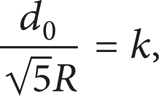
Set

$\hspace{0.17em}{t}_{\text{work}}\left(j\right)=T_{\text{collect}}.$

(18)

If setting k = N _j , then

$t_{\text{sleep}}\left(j\right)=N_j{T}_{\text{collect}}-T_{\text{collect}}=\left(N_j-\mathrm{1}\right)t_{\text{work}}\left(j\right).$

(19)

When there are 2 nodes in A _j , the scheduling cycle in A _j is 2 T_collect while each node works and sleeps for T_collect time in turn. When there are 3 nodes in A _j , the scheduling cycle in A _j is 3 T_collect, and each node will work for T_collect time and sleep for 2 T_collect time in turn. If a node in A _j dies, N _j will be minus 1.

The procedure of node sleep scheduling is described as in Algorithm 2.

Algorithm 2:

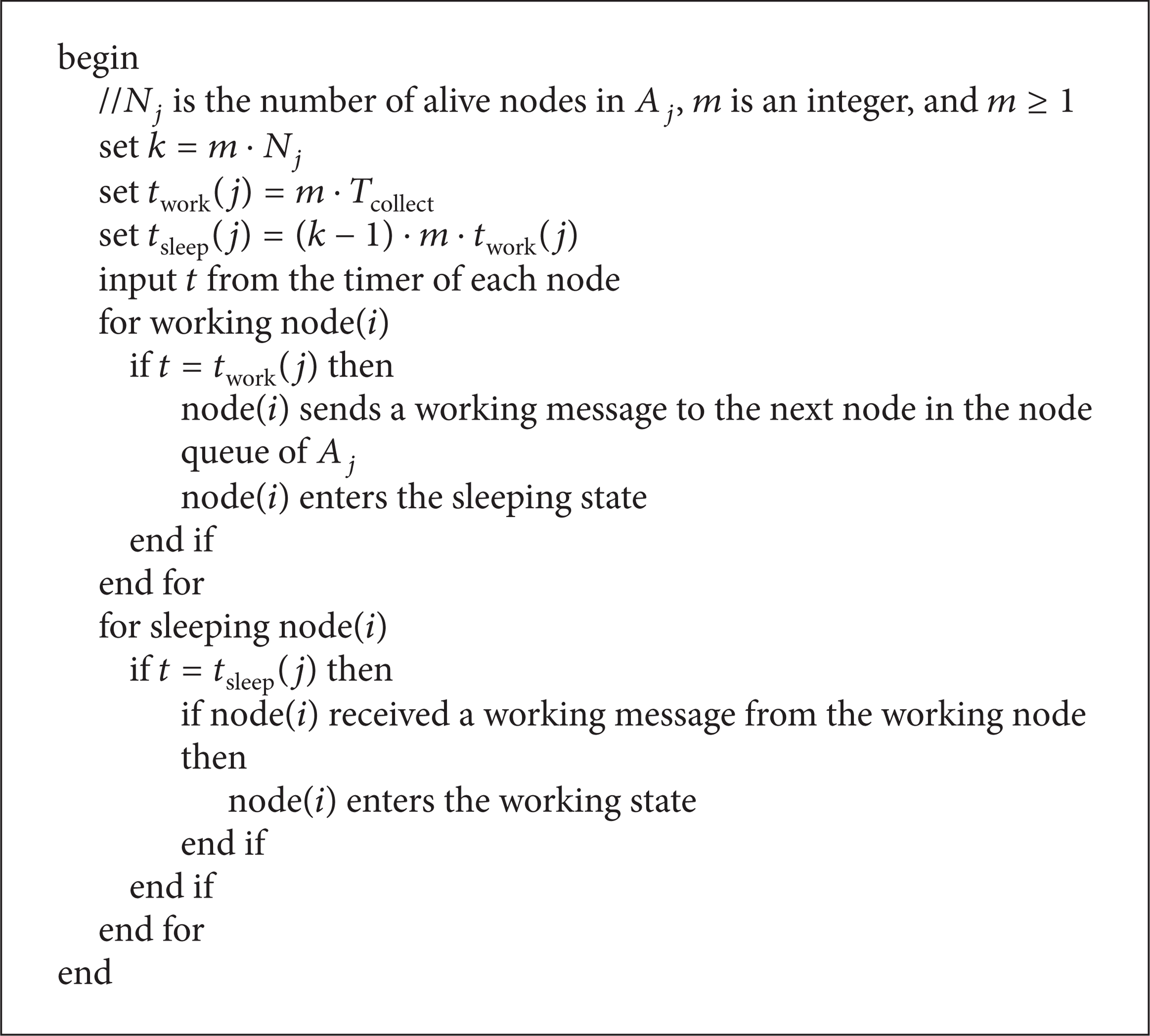
The procedure of node sleeping scheduling in A _j .

5.2. Enhancing Robustness to Partial Occlusion

The most important role of WSNs deployed to monitor situations in the environment is to report emergency incidents to the BS. The working node in a region can perceive events when a moving target enters the region, such as a spreading gas leak or fire. If the detected value is above a threshold, the network should send an alarm to the BS as soon as possible. At the same time, the working node will send an assisting message to wake other nodes up in the grid to precisely track the whole journey of the target (a moving object, gas, or fire). To avoid waking up nodes in other grids by mistake, the assisting message contains information on the partition's ID. The sleeping nodes enter the assisting state after being woken up by the working node and begin to trace the event. When the working node has worked for t_work(j) time, the working node sends a working message to the next node in the node queue and the working node enters the assisting state. The next node in the node queue will switch to the working state after receiving the working message.

Wakeup scheduling leads to increased energy consumption compared to sleep scheduling. But this does not mean that energy is wasted. However, saving energy will lengthen the effective working lifetime of the network. The intention behind wakeup scheduling is to get accurate detection information. The redundant nodes will sleep again when the unusual event disappears from the local grid.

When a target enters a grid or some other unusual events occur in the grid, the working node in other grids might perceive the target as shown in Figure 13. The nodes in other grids are woken up to the assisting state, but some of them might not perceive the target because the target has not entered their range of perception or has moved far away. To save energy in such cases, a node will enter the sleeping state again if its sensor value is below a threshold after a time interval δ. As shown in Figure 14, all assisting nodes in the grid returned to the sleeping state after time δ (=5 s). This strategy reduced the system overhead, while continuing the precise tracking of the target.

Figure 13:

An example of wakeup scheduling.

Figure 14:

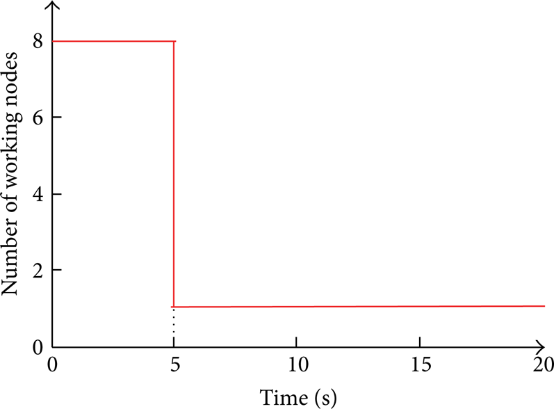
Nodes in the assisting state go back to the sleeping state after period δ (=5 s) in grid A _j .

The procedure of node wakeup scheduling is described as in Algorithm 3.

Algorithm 3:

The procedure of node wakeup scheduling in A _j .

5.3. The State-Transition of the Proposed Scheduling Approach

The whole process of the proposed algorithm can be illustrated by the state-transition shown in Figure 15.

Figure 15:

Diagram of the state-transition of each node.

Scheduling is simple. Each node needs to maintain the state of its neighbor nodes. The node transits states only according to the cycle and wakes other nodes up according to the node queue. In the beginning, each node is in the sleeping state. Each node enters the initializing state only once to initialize and start the network. Then, the node is switched to different operation states until it dies. The node is in one state at a time of sleeping, working, and assisting. t_work(j) will change with the node's death in A _j . Only N _j and the node queue need to be maintained.

6. Simulation Results

The algorithm was simulated with MATLAB. The parameters used in the simulation are shown in Table 1. There are 2500 nodes randomly distributed in an area of 80 × 80 m². Each node has the same structure. The sensor parameters refer to the parameters of the chip Ti CC2533. The power consumed by the node in the transmission, reception, idle, and sleep modes is 572009 mW, 42 mW, 0.4 mW, and 0.03 mW, respectively. The initial energy of a node is randomly chosen from the range of 54–60 Jules to simulate the variance in battery lifetimes. The sensing range R _p is 3 meters, and R _t is 10 meters.

Table 1:

The main parameters used in simulation.

Parameter	Value
Object region	80 × 80 m2
Node number	500, 1000, 1500, 2000, 2500
Initial energy	54∼60 Jules
E elec	5 nJ/bit
εfs	10 pJ/bit/m2
εmp	0.0013 pJ/bit/m4
d 0	87 m

A source and a sink are placed in opposite corners of the field. The source generates a data report every 10 seconds and the data report is delivered to the sink. In the simulation, we compared our method with PEAS. The GRAB forwarding protocol [7] is used in the simulation for PEAS. The simulation of our scheduling algorithms is based on the EEC proposed in this paper. We test the effective lifetime of the network, which is the duration during which the data can be successfully delivered to the sink rather than the absolute lifetime of the network.

6.1. Simulation Results of Sleep Scheduling

The grid was built to be R = 3.82 m, R = 2.97 m, and R = 2.23 m, respectively, where 3.82 m is approximate to $\sqrt{\mathrm{2}}{R}_p$ and 2.23 m is approximate to $\sqrt{\mathrm{2}}{R}_p$ /2. The node failure rate λ = 0.01, and data acquisition cycle T_collect = 50 s. Therefore, we set t_work = 50 s and t_sleep = (N _j − 1) × 50 s.

6.1.1. Test of Network Coverage

The network coverage of PEAS and the proposed algorithm are shown in Figure 16. In this simulation, the network scale is 2000 nodes. The value of R in the proposed method directly affected the network coverage. As shown in Figure 16, at 2 × 10⁴ seconds, the network cannot achieve full coverage both in PEAS and in the proposed algorithm with R = 2.23 m, while the network can achieve full coverage by applying the proposed algorithm with R = 3.82 m and R = 2.97 m. The coverage of the proposed algorithm is always 100% before 4 × 10⁴ seconds with R = 3.82 m. At 4 × 10⁴ seconds, the coverage of the proposed algorithm with R = 2.23 m is twice that of PEAS. After 4 × 10⁴ seconds, the network cannot work with PEAS while our method can still maintain high network coverage if a suitable value is selected for R.

Figure 16:

A comparison of network coverage for different strategies.

The network coverage of PEAS decreases greatly as the nodes die. For the proposed scheduling, the network coverage decreases more quickly when R is small because more nodes die at a certain time than is the case with a bigger R. Hence, a small R promises a better network coverage than a big R if the death of nodes is not taken into consideration. However, in real applications, the death of nodes has to be taken into account. Therefore, it is not the case that the smaller the R, the better the coverage. As the simulation results show, in applying our method, the network coverage is best when $R\approx \sqrt{\mathrm{2}}{R}_p$ .

6.1.2. Test of Effective Lifetime

Achieving better coverage requires getting more nodes to keep on working; however, setting more nodes in the working state will shorten the lifetime of the network. A balance between the two conditions needs to be found. Figures 17 and 18 show the performances of proposed scheduling algorithms based on EEC and performances of PEAS based on GRAB.

Figure 17:

Network effective lifetime versus network scale for different strategies.

Figure 18:

Effective lifetime versus failure rate.

Figure 17 illustrates the results of the simulation of effective lifetime when the network scale was 500, 1000, 1500, 2000, and 2500 nodes, respectively. When there were 2500 nodes in WSN, the network could not work at about 2.1 × 10⁴ seconds with the application of PEAS, while the network effective lifetime of the proposed algorithm with R = 2.23 m reached about 2.5 × 10⁴, and the network effective lifetime of the proposed algorithm when R = 2.97 m and R = 3.82 m was 3.7 × 10⁴ and 5 × 10⁴, respectively. This shows that the network can work for the longest time when we apply our method when $R\approx \sqrt{\mathrm{2}}{R}_p$ , compared to PEAS and to our method with a smaller R.

Figure 18 shows the effective lifetime under various failure rates from 25 to 250 per 5000 seconds when the network scale is 2500. When we take the failure rate into account, our method guarantees the longest effective lifetime when $R\approx \sqrt{\mathrm{2}}{R}_p$ compared to PEAS and our method with a smaller R. As the failure rate increases, the lifetime tends to decrease. The effective lifetime of PEAS decreases about 25% when the failure rate is 250. The network effective lifetime is approximately stable when the proposed method is applied with any R, even in the case of the biggest failure rate.

6.2. Simulation Results of Wakeup Scheduling

The time threshold in the simulation of the event-driven mode was set as δ = 5 s. Figure 19 illustrates all of the assisting nodes that were woken up along the target trail when the grid was built with R = 3.82 m. The target entered the monitoring area at the lower-left corner, crossed the monitoring area, and left at the upper-right corner. As shown in Figure 19, there are enough nodes to perceive the target so that the target will not be lost.

Figure 19:

Nodes woken up along the target trace.

To clearly observe the node states, the distribution of assisting nodes in the monitoring area is shown in Figure 20. The working node in grid A₁₃₆ woke up all sleeping nodes in this region. The nodes will not perceive the target until it moves far away from them.

Figure 20:

Distribution of assisting nodes in the monitoring area.

7. Conclusion

An energy efficient data routing approach based on tier division was first proposed. Based on EEC, a hybrid node scheduling approach based on partition was proposed. The scheduling can reduce energy consumption while reaching the goals of both time-driven and event-driven applications. The results of the simulation show that the sleep scheduling can efficiently and reliably prolong the effective lifetime of WSN and the wakeup scheduling can trace events with precision. Moreover, the method has very good time performance for real applications because it is very simple. Hence, the proposed algorithm can be applied to complex real applications that demand not only the periodic collection of information but also the tracking of unusual events.

Conflict of Interests

The authors declare that there is no conflict of interests regarding the publication of this paper.