Rapid Evaluation for Position-Dependent Dynamics of a 3-DOF PKM Module

Abstract

Based on the substructure synthesis and modal reduction technique, a computationally efficient elastodynamic model for a fully flexible 3-RPS parallel kinematic machine (PKM) tool is proposed, in which the frequency response function (FRF) at the end of the tool can be obtained at any given position throughout its workspace. In the proposed elastodynamic model, the whole system is divided into a moving platform subsystem and three identical RPS limb subsystems, in which all joint compliances are included. The spherical joint and the revolute joint are treated as lumped virtual springs with equal stiffness; the platform is treated as a rigid body and the RPS limbs are modelled with modal reduction techniques. With the compatibility conditions at interfaces between the limbs and the platform, an analytical system governing differential equation is derived. Based on the derived model, the position-dependent dynamic characteristics such as natural frequencies, mode shapes, and FRFs of the 3-RPS PKM are simulated. The simulation results indicate that the distributions of natural frequencies throughout the workspace are strongly dependant on mechanism's configurations and demonstrate an axial-symmetric tendency. The following finite element analysis and modal tests both validate the analytical results of natural frequencies, mode shapes, and the FRFs.

1. Introduction

The concept of parallel kinematics allows the design of manipulators that combines high stiffness properties with lightweight structures, which leads to potentially superior dynamic behaviors. Based on the principle of parallel kinematics, machining tool with two to six degrees of freedom (DOFs) can be realized through different kinematic designs. This makes PKM tools a promising alternative solution for high-speed machining of extra large scale components with complex geometries.

This proposition has been fully exemplified by the commercial success of Tricept robot [1] and Sprint Z3 head [2] applied in aeronautical industries. Considering the priority of the PKM, the authors presented a newly invented PKM module named the A3 head [3]. It is a novel 3-RPS PKM module that is proposed with one translational and two rotational capabilities. Added by an x-y motion platform, this module can be used as a multiple-axis spindle head to form a hybrid 5-axis high-speed machine (HSM) tool.

Dynamics model considering the structure flexibility is one of the most overwhelming concerns in the earlier performance prediction and the later utility of such a PKM when it is used for HSM applications. The process-machine interactions are influenced by the dynamic stiffness between the tool center point (TCP) and the workpiece, which determines the maximum depth of cut due to chatter constraints [4]. The dynamic stiffness at the TCP and the maximum stable depth of cut are further influenced by the system's tool—toolholder-spindle configuration and the dynamic behavior of the machine structure, which depends strongly on the position of the moving platform in the workspace for PKM tools [5, 6]. The structural dynamics of the 3-RPS based machine tool is also position varying as the tool moves along the tool path [7, 8]. There have been lots of references about the TCP FRF evaluation of the tool—toolholder-spindle configuration [9–12]. However, rapid evaluation for the position-dependent FRFs based on structure dynamics of PKM tools is still a huge challenge.

Finite element method (FEM) is commonly used for the dynamic modeling of PKMs due to their complex geometries. Investigation based on a “virtual prototyping” technique using FEM model of the machine is an alternative solution [13]. However, structure dynamic analyses for full machine finite element models, which are typically on the order of 1,000,000 DOFs or more, are computationally expensive [14, 15]. Therefore, the analytical or semianalytical dynamic modeling method is needed for rapid evaluation.

In the structural dynamics literature, substructure synthesis techniques have been investigated intensively and applied widely [16]. Substructure synthesis technique, also known as component mode synthesis (CMS) method, can be used to model flexible components using FEM and then to assemble these component models to model the dynamic behavior with a relatively small number of DOFs. A simplified FEM based on the CMS is used to deal with the dynamic modeling problem of 6-RPR spatial parallel manipulators by modeling the limbs using spatial beam elements [17]. Piras et al. [18] established an elastodynamic model of a 3-PRR flexible-link planar parallel platform in similar manner, including the mapping of the first-order natural frequency with respect to the robot configuration. On the assumption that the deformations of the intermediate links are small relative to the length of the links, Zhang et al. [19] presented a structural dynamic model for the 3-PRR flexible parallel manipulator using the CMS. The experimental modal tests were performed to validate the theoretical model through comparison of the dynamic characteristics. With substructure synthesis techniques, Zhou et al. [20, 21] provided a fully flexible 3-PRS manipulator vibration model in which the links were modeled as finite elements. The system's natural frequencies and the FRFs were compared between the simulation results and the experiments. An elastodynamic model of the 8-PSS flexible redundant parallel manipulator was developed by using the finite element method and the substructure synthesis technique [22], with which the sensitivity analysis of the dynamic characteristics represented by the natural frequency was conducted.

In the PKM tools field, the stability is closely related to the structure dynamic characteristics [13, 23]. Hong et al. [24] derived a vibration model for a 6-DOF PKM tool, in which the rods of the PKM were considered as spring-damper systems. They performed stability analysis through a combination of the regenerative cutting and the position-dependent dynamics. Pedrammehr et al. [25] studied the dynamic characteristics of a Stewart platform-based machine tool table by taking the damping and stiffness of the rods into account. In this paper, the impact of position and orientation of the moving platform on dynamic behavior as well as forced vibrations of the moving platform by the milling force were studied to present the proper configurations of the moving platform in different machining condition. Henninger and Eberhard [6, 26] proposed a dynamic modeling for a 6-DOF hexapod machine tool named Paralix with substructure synthesis technique. With the proposed model, the stability diagrams for milling processes were investigated and pose-dependent stability diagrams for two example trajectories are presented. Law et al. [7] modeled the position-dependent FRFs of a hybrid serial-parallel kinematic machine tool by synthesizing its substructural reduced order finite element models, and the stability maps were simulated as a function of machine positions.

In the literatures cited above, most of the researchers focused on the dynamic characteristics of the parallel manipulators or the parallel robotics. The investigation on the dynamic response used for the stability analysis of high-speed PKM tools is relatively less. It should also be pointed out that the limbs of the PKM in the dynamic model above were simplified as spatial beam elements or spring system despite their complex geometries. In addition, the joint compliances in most of the models were not taken into account though they would bring significant bearings on the stiffness of the system [27].

This paper presents a dynamic model and then conducts a position-dependent dynamic analysis for a 3-RPS PKM, which can be used for the stability analysis of the high-speed machine tool. The analysis results are validated through a comparison between the simulation and the experimental results. The remainder of the paper is organized as follows. At first, kinematic modeling for the 3-RPS is described in Section 2. Dynamic modeling of substructures of the 3-RPS is presented in Section 3 followed by joint stiffness and substructure synthesis in Section 4. A virtual prototype model to demonstrate the position-dependent dynamic characteristics is compared with experimental results in Section 5. At last, some conclusions are drawn in Section 6.

2. Kinematic Modeling

2.1. Structural Description

Figure 1 shows a CAD model of the A3 head, which consists of a moving platform, a base, and three identical RPS limbs. Herein, R and S represent a revolute and spherical joint, and the underlined P stands for an active prismatic joint, respectively. Independently driven by 3 servomotors, one translation along z-axis and two rotations about x- and y-axes can be achieved. An electrical spindle can be mounted on the moving platform to implement high-speed milling.

Figure 1:

Structure of the 3-RPS module.

The three RPS limbs of the A3 head are axially symmetrically distributed, and the mechanical features can be addressed in brief as follows.

1. The revolute joint is designed as a closed frame. Two opposing short half-shafts project from the frame, rigidly fixed to the inner rings of bearings that have outer rings mounted within block units attached to the base by bolts and pins. Internally, each side of the closed frame carries two sliding blocks of a ball guideway; the slideways are mounted on each side of the limb body. The closed frame also carries the nut of the lead-screw assembly.

2. The limb body carries a servomotor and lead-screw thrust bearing at the rear and a spherical bearing at the tip. The limb body is a hollow rectangular structure having inner stiffeners, dished on one side to accommodate the lead-screw. Its cross-section dimensions are set to keep overall sizes and weight as low as practicable while providing adequate rigidity.

3. The spherical joint is designed as a combination of three revolute joints with their axes being orthogonal to one another, connecting the moving platform to the limbs for force transmission.

2.2. Coordinate Systems

Figure 2 shows the schematic diagram of the A3 head, where A _i (i = 1, 2, 3) is the center of the spherical joint of the ith limb; B _i (i = 1, 2, 3) is the center of the revolute joint; C _i (i = 1, 2, 3) is the center of the servomotor. The moving platform ΔA₁A₂A₃ and the base ΔB₁B₂B₃ are set to be equilateral triangles with A and B being the center point, respectively. A reference coordinate system B − x _B y _B z _B is attached to point B, with the axes direction shown in Figure 2; a body fixed coordinate system A − uvw is placed at point A, paralleling to the coordinate system B − x _B y _B z _B at its initial position; A _t is the tool tip point, with w _t being the position vector in the coordinate system A − uvw; a limb reference frame B _i − x _i y _i z _i is established at the center point of B _i (i = 1, 2, 3) of the ith revolute joint, with x _i and z _i being coincided with the axes of revolute joint and the limb, respectively, while y _i is directed by right hand rule. s_1i (i = 1, 2, 3) is the revolute axes of the ith limb of the A3 head, with s₁₁ being coincided with x _B ; s_2i (i = 1, 2, 3) is the unit vector of the prismatic joint of the ith limb; q _i (i = 1, 2, 3) is the ith limb length between the spherical joint and the revolute joint. Each limb is divided into n − 1 elements, with n nodes totally. The nodes reference frame N _ij − x _ij y _ij z _ij (i = 1, 2, 3, j = 1, 2,…, n) is set at the jth node of the ith limb paralleling to the B _i − x _i y _i z _i .

Figure 2:

Schematic diagram of the 3-RPS PKM.

The transformation matrix of the frame A − uvw with respect to the frame B − x _B y _B z _B can be formulated as

$\mathbf{R}=\text{Rot}\left(z,\psi \right)\text{Rot}\left(x,\theta \right)\text{Rot}\left(z,\varphi \right)=\left[\begin{array}{ccc}c\psi c\varphi -s\psi c\theta s\varphi & -c\psi s\varphi -s\psi c\theta c\varphi & s\psi s\theta \\ s\psi c\varphi +c\psi c\theta s\varphi & -s\psi s\varphi +c\psi c\theta c\varphi & -c\psi s\theta \\ s\theta s\varphi & s\theta c\varphi & c\theta \end{array}\right],$

(1)

where s = sin, c = cos, and ψ, θ, and ϕ are three Euler angles of precession, nutation, and body rotation, respectively.

The orientation matrix of the limb frame B _i − x _i y _i z _i with respect to frame B − x _B y _B z _B is

${\mathbf{R}}_i=\text{Rot}\left(z,{\varphi }_i\right),\hspace{1em}i=\mathrm{1,2},\mathrm{3},$

(2)

where ϕ₁ = 0, ϕ₂ = 2π/3, and ϕ₃ = 4π/3.

The position vector r _Ai of point A _i with respect to the frame B − x _B y _B z _B can be expressed by

${\mathbf{r}}_{A_i}={\mathbf{r}}_A+{\mathbf{a}}_i,\hspace{1em}i=\mathrm{1,2},\mathrm{3},$

(3)

where a _i = Ra_i0, a_i0 represent the vector of point A _i measured in A − uvw, r _A is the position vector of point A with respect to B − x _B y _B z _B , and

${\mathbf{r}}_A={\mathbf{b}}_i+q_i{\mathbf{s}}_{\mathrm{2}i}-{\mathbf{a}}_i.$

(4)

Taking ψ, θ and a as independent coordinates, and considering the constraints of revolute joint, we obtain the ${\mathbf{r}}_A={(r_{Ax}\hspace{1em}{r}_{Ay}\hspace{1em}{r}_{Az})}^{\text{T}}$ as follows:

$\begin{array}{c}{r}_{Ax}=\frac{a\left(\mathrm{1}-\cos \theta \right)\sin \mathrm{2}\psi }{\mathrm{2}},\\ r_{Ay}=\frac{a\left(\mathrm{1}-\cos \right)\cos \mathrm{2}\psi }{\mathrm{2}},\\ \varphi =-\psi .\end{array}$

(5)

Equation (5) gives the parasitic motions of the 3-RPS mechanism. Using (1), (4), and (5), the inverse position analysis can be conducted as follows:

$\begin{array}{c}{q}_i=\left|{\mathbf{r}}_A+{\mathbf{a}}_i-{\mathbf{b}}_i\right|\\ {\mathbf{s}}_{\mathrm{2}i}=\frac{\left(\mathbf{r}+{\mathbf{a}}_i-{\mathbf{b}}_i\right)}{q_i},\hfill \\ \hspace{1em}\hspace{1em}i=\mathrm{1,2},\mathrm{3}.\end{array}$

(6)

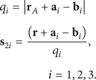
The vector s_2i measured in frame B _i − x _i y _i z _i is

${}^{B_i}{\mathbf{s}}_{\mathrm{2}i}={\mathbf{R}}_i^{-\mathrm{1}}{\mathbf{s}}_{\mathrm{2}i}={\left(\begin{array}{ccc}{}^{B_i}{s}_{\mathrm{2}ix}& {}^{B_i}{s}_{\mathrm{2}iy}& {}^{B_i}{s}_{\mathrm{2}iz}\end{array}\right)}^{\text{T}},$

(7)

${\theta }_i=\arctan \left(-\frac{{}^{B_i}{s}_{\mathrm{2}iy}}{{}^{B_i}{s}_{\mathrm{2}iz}}\right),\hspace{1em}i=\mathrm{1,2},\mathrm{3},$

(8)

where θ _i is the revolute angle of the ith limb.

The node N _ij of the ith limb measured in the frame B _i − x _i y _i z _i is

$\begin{array}{c}{\mathbf{l}}_{Nij}=\{\begin{array}{cc}{\left[\begin{array}{ccc}\mathrm{0}& \mathrm{0}& q_i-{\displaystyle \sum }_j^{n-\mathrm{1}}{l}_{ij}\end{array}\right]}^{\text{T}}\hfill & j=\mathrm{1,2},\dots ,n-\mathrm{1}\hfill \\ {\left[\begin{array}{ccc}\mathrm{0}& \mathrm{0}& q_i\end{array}\right]}^{\text{T}}\hfill & j=n,\hfill \end{array}\\ i=\mathrm{1,2},\mathrm{3}.\end{array}$

(9)

The position vector l _Nij measured in the frame B − x _B y _B z _B can be expressed as

${}^B{\mathbf{l}}_{Nij}={\mathbf{R}}_i\text{Rot}\left(x,{\theta }_i\right){\mathbf{l}}_{Nij}+{\mathit{b}}_i.$

(10)

The detailed derivation process of the 3-RPS module was addressed in our previous work [3].

3. Dynamic Modeling of the Substructures of the 3-RPS

With the substructure synthesis technique and the previous kinematic analysis, the 3-RPS PKM is divided into a moving platform substructure and 3 identical RPS limb substructures. The following hypotheses and approximations are made during the dynamic modeling process.

1. The base and the moving platform are treated as rigid bodies.

2. Based on the modal reduction techniques, the limbs’ bodies are modelled by importing CAD model into the finite element software for preprocessing and are then reduced into spatial beam structures.

3. The compliances of revolute and spherical joints are simplified as lumped virtual springs with equivalent stiffness.

4. The coupling effect between rigid and elastic motions is negligible as the mechanism works at low or moderate speed.

5. A structural damping is considered in the position-dependence FRF analysis.

6. Clearances in joint are all neglected.

3.1. Substructure Modal Reduction

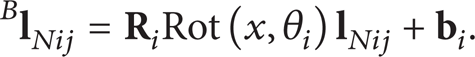
Figure 3 shows the assembly of a RPS limb in which l is total length of the limb, q _i is limb length between the center point of spherical and revolute joint, l _n is the distance from nut to center of the revolute joint.

Figure 3:

Assembly of a RPS limb.

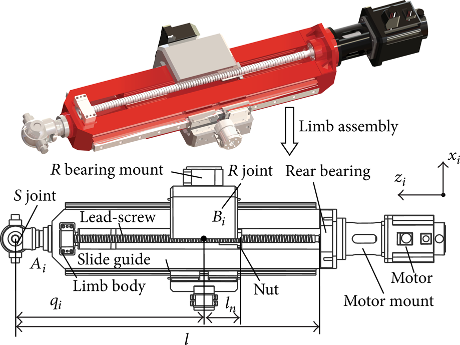
Considering both computational efficiency and accuracy, the modal reduction technique is used to complete the limb elastodynamic modeling. Figure 4 is the limb substructure modal reduction diagram. An FE model for limb substructure was generated from its detailed CAD model using solid elements by the ANSYS software. The structural component was assigned material properties as modulus of elasticity of 206 GP, density of 7850 kg/m³, and Poisson's ratio of 0.25. After necessary convergence tests of the FE model, the substructural system matrices were exported to the MATLAB environment. The following subsequent modal reduction and substructure synthesis were conducted within the MATLAB environment.

Figure 4:

Limb substructural model reduction.

In Figure 4, A _i and C _i are the endpoints of the limb and represent the center point of the spherical joint and servomotor, respectively. B _i is the virtual condensation node, which is used to connect the interface nodes within the closed frame by interpolation multipoint constraints (MPC) formulation [28]. u _B and u _E represent the DOFs of the virtual node B _i and the nodes within the closed frame, respectively.

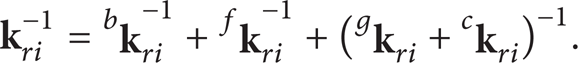
The dynamical equations of the limb from the FE model can be expressed as follows:

$\mathbf{m}\ddot{\mathbf{u}}+\mathbf{k}\mathbf{u}=\mathbf{f},$

(11)

where m and k are mass and stiffness matrices and u and f are the general coordinates vector and external load vector. The characteristic equation of (11) is

$\mathbf{k}\mathbf{\Phi }=\mathbf{m}\mathbf{\Phi }\mathrm{\Lambda },$

(12)

where Λ and Φ are eigenvalue and eigenvector matrices, respectively. Since the reduction procedure involves eliminating a subset of DOFs from u , the system matrices are partitioned into reserved DOFs u _a and reduced DOFs u _b as

$\left[\begin{array}{cc}{\mathbf{k}}_{aa}& {\mathbf{k}}_{ab}\\ {\mathbf{k}}_{ba}& {\mathbf{k}}_{bb}\end{array}\right]\left\{\begin{array}{c}{\mathbf{\Phi }}_a\\ {\mathbf{\Phi }}_b\end{array}\right\}=\left[\begin{array}{cc}{\mathbf{m}}_{aa}& {\mathbf{m}}_{ab}\\ {\mathbf{m}}_{ba}& {\mathbf{m}}_{bb}\end{array}\right]\left\{\begin{array}{c}{\mathbf{\Phi }}_a\\ {\mathbf{\Phi }}_b\end{array}\right\}\mathrm{\Lambda }.$

(13)

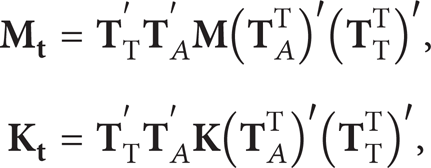
According to the conservation law of kinetic energy and potential energy, the reduced mass and stiffness matrices can be obtained as follows:

$\begin{array}{c}{\mathbf{m}}_r={\mathbf{m}}_{aa}+{\mathbf{m}}_{ab}{\mathbf{T}}_r+{\mathbf{T}}_r^{\text{T}}{\mathbf{m}}_{ba}+{\mathbf{T}}_r^{\text{T}}{\mathbf{m}}_{bb}{\mathbf{T}}_r,\\ {\mathbf{k}}_r={\mathbf{k}}_{aa}+{\mathbf{k}}_{ab}{\mathbf{T}}_r+{\mathbf{T}}_r^{\text{T}}{\mathbf{k}}_{ba}+{\mathbf{T}}_r^{\text{T}}{\mathbf{k}}_{bb}{\mathbf{T}}_r,\end{array}$

(14)

where m _r and k _r are reduced mass and stiffness matrices, respectively, and ${\mathbf{T}}_r={\mathit{\Phi }}_a{\mathit{\Phi }}_{\mathit{b}}^{-\mathit{1}}$ is the transformation matrix for reduction.

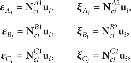
As the limb length q _i is changing with the position and posture of the A3 head, a different set of nodes of limb comes into contact with the revolute joint. The substructures will be incompatible for the further assembling of substructure models [7, 14]. As shown in Figure 4, to make the incompatible substructure synthesis possible, a virtual condensation node B _i representing only a subset of interface nodes within the closed frame is defined; all interface nodal DOFs u _E are represented by the condensation node DOFs u _B using constraint equations without any interface reduction. The interface nodal DOFs u _E can be expressed as

${\mathbf{u}}_E={\mathbf{N}}_E{\mathbf{u}}_a,$

(15)

where N _E is transformation matrix.

The interpolation MPC formulation defines displacements and rotations of the condensation node as the weighted average of the motion of the interface nodes in contact. The motions of the condensation node DOFs u _B are fully described by the displacement of the interface nodes DOFs u _E in contact as [28]

${\mathbf{\epsilon }}_B=\frac{{\sum }_{k=\mathrm{1}}^p{w}_k{\mathbf{u}}_{Ek}}{{\sum }_{k=\mathrm{1}}^p{w}_k},\hspace{1em}\hspace{1em}{\mathbf{\xi }}_B=\frac{{\sum }_{k=\mathrm{1}}^p{w}_k{\mathbf{r}}_{Bk}\times {\mathbf{u}}_{Ek}}{{\sum }_{k=\mathrm{1}}^p{w}_k{\left|{\mathbf{r}}_{Bk}\right|}^{\mathrm{2}}},$

(16)

where ε _B and ξ _B represent the linear and angular DOFs of virtual node B _i ; u _Ek is the kth node DOFs of the interface nodes. To ensure that the condensation node represents the average motion of the contacting interface, the weight factors w _k for each DOF are chosen proportional to the part of the interface area that its node represents, as shown in [14]. r _Bk is the position vector from B _i to the kth node. Equation (16) can be expressed as

${\mathbf{u}}_B={\mathbf{T}}_C{\mathbf{u}}_E,$

(17)

where T _C is the transformation matrix. And ${\mathbf{u}}_B={[{\mathit{\epsilon }}_B^{\text{T}}\hspace{1em}{\mathbf{\xi }}_B^{\text{T}}]}^{\text{T}}$ . Herein

$\begin{array}{c}{\mathbf{T}}_C=\left[\begin{array}{cccc}{\mathbf{T}}_{C\mathrm{1}}& {\mathbf{T}}_{C\mathrm{2}}& \begin{array}{ccc}\cdots & {\mathbf{T}}_{Ck}& \cdots \end{array}& {\mathbf{T}}_{Cp}\end{array}\right],\\ {\mathbf{T}}_{Ck}=\left[\begin{array}{cc}{\mathbf{T}}_{Ck\mathrm{11}}& {\mathbf{0}}_{\mathrm{3}\times \mathrm{3}}\\ {\mathbf{T}}_{Ck\mathrm{21}}& {\mathbf{0}}_{\mathrm{3}\times \mathrm{3}}\end{array}\right],\hspace{1em}k=\mathrm{1,2},\dots ,p,\\ {\mathbf{T}}_{Ck\mathrm{11}}=\mathrm{diag}\left(\begin{array}{ccc}{w}_{Ck}& w_{Ck}& w_{Ck}\end{array}\right),\hspace{1em}\hspace{1em}{w}_{Ck}=\frac{w_k}{{\sum }_{k=\mathrm{1}}^p{w}_k},\\ {\mathbf{T}}_{Ck\mathrm{21}}=\frac{w_k}{{\sum }_{k=\mathrm{1}}^p{w}_k{\left|r_{Bk}\right|}^{\mathrm{2}}}\left[\begin{array}{ccc}\mathrm{0}& -r_{Bkz}& r_{Bky}\\ r_{Bkz}& \mathrm{0}& -r_{Bkx}\\ -r_{Bky}& r_{Bkx}& \mathrm{0}\end{array}\right].\end{array}$

(18)

3.2. Dynamic Model of the RPS Limb

During the elastodynamic modeling process for the RPS limb, the spherical and revolute joints are treated as virtual lumped springs-damping system with equal stiffness and damping coefficient; servomotor is simplified as lumped rigid body. Consequently, the entire limb can be modeled as a spatial beam supported by two sets of lumped springs-damping systems as shown in Figure 5.

Figure 5:

Force diagram of limb.

Herewith, k _sxi , k _syi , and k _szi are the stiffness coefficients of three virtual transverse linear springs of the spherical joint, and c _sxi , c _syi , and c _szi are the damping coefficients; k_r1xi, k_r1yi, k_r1zi, k_r2xi, k_r2yi, and k_r2zi are stiffness coefficients of the transverse and torsional springs of the revolute joints, and c_r1xi, c_r1yi, c_r1zi, c_r2xi, c_r2yi, and c_r2zi are the damping coefficients accordingly.

Based on (11) and (14), a set of dynamical equations of ith limb in the limb frame B _i − x _i y _i z _i is formulated with adequate boundary conditions. For convenience, the subscript except the limb number i (1, 2, 3) is neglected:

${\mathbf{m}}_i{\ddot{\mathbf{u}}}_i+{\mathbf{c}}_i{\dot{\mathbf{u}}}_i+{\mathbf{k}}_i{\mathbf{u}}_i={\mathbf{f}}_i,$

(19)

where m _i , c _i , and k _i are the reduced mass, damping, and stiffness matrices, respectively. u _i , f _i are the general coordinates vector and external load vector of the ith limb and can be expressed as follows:

$\begin{array}{c}{\mathbf{u}}_i=\left\{\begin{array}{c}{\mathbf{\epsilon }}_{in}\\ {\mathbf{\xi }}_{in}\\ ⋮\\ {\mathbf{\epsilon }}_{ij}\\ {\mathbf{\xi }}_{ij}\\ ⋮\\ {\mathbf{\epsilon }}_{i\mathrm{1}}\\ {\mathbf{\xi }}_{i\mathrm{1}}\end{array}\right\},\hspace{1em}\hspace{1em}{\mathbf{f}}_i=\left\{\begin{array}{c}{\mathbf{f}}_{in}\\ {\mathit{\tau }}_{in}\\ ⋮\\ {\mathbf{f}}_{ij}\\ {\mathit{\tau }}_{ij}\\ ⋮\\ {\mathbf{f}}_{i\mathrm{1}}\\ {\mathit{\tau }}_{i\mathrm{1}}\end{array}\right\},\\ i=\mathrm{1,2},\mathrm{3}\hspace{1em}j=\mathrm{2,3},\dots ,n-\mathrm{1}.\end{array}$

(20)

Make the DOFs ε _in = ε _Ai , ξ _in = ξ _Ai , ε _ij = ε _Bi , ξ _ij = ξ _Bi , ε_i1 = ε _Ci , ξ_i1 = ξ _Ci , f _in = f _PLi , f _ij = f _BLi , and τ _ij = τ _BLi . Herein ε _Ai , ξ _Ai , ε _Bi , ξ _Bi , ε _Ci , and ξ _Ci are the linear and angular DOFs of the nodes A _i , B _i , and C _i in B _i − x _i y _i z _i ; f _PLi , f _BLi , and τ _BLi are reaction forces and moments at nodes A _i and B _i measured in B _i − x _i y _i z _i , respectively. The nodal coordinates can be related to u _i as follows:

$\begin{array}{c}{\mathbf{\epsilon }}_{A_i}={\mathbf{N}}_{ci}^{A\mathrm{1}}{\mathbf{u}}_i,\hspace{1em}\hspace{1em}{\mathbf{\xi }}_{A_i}={\mathbf{N}}_{ci}^{A\mathrm{2}}{\mathbf{u}}_i,\\ {\mathbf{\epsilon }}_{B_i}={\mathbf{N}}_{ci}^{B\mathrm{1}}{\mathbf{u}}_i,\hspace{1em}\hspace{1em}{\mathbf{\xi }}_{B_i}={\mathbf{N}}_{ci}^{B\mathrm{2}}{\mathbf{u}}_i,\\ {\mathbf{\epsilon }}_{C_i}={\mathbf{N}}_{ci}^{C\mathrm{1}}{\mathbf{u}}_i,\hspace{1em}\hspace{1em}{\mathbf{\xi }}_{C_i}={\mathbf{N}}_{ci}^{C\mathrm{2}}{\mathbf{u}}_i,\end{array}$

(21)

where N _ci ^A1, N _ci ^A2, N _ci ^B1, N _ci ^B2, N _ci ^C1, and N _ci ^C2 are connectivity matrices of nodes A _i , B _i , and C _i with respect to u _i in B _i − x _i y _i z _i , respectively. As the node B _i is virtual condensation node, the N _ci ^B1 and N _ci ^B2 can be expressed as

$\begin{array}{c}{\mathbf{N}}_{ci}^{B\mathrm{1}}={\mathbf{T}}_{B\mathrm{1}}{\mathbf{T}}_C{\mathbf{N}}_E,\\ {\mathbf{N}}_{ci}^{B\mathrm{2}}={\mathbf{T}}_{B\mathrm{2}}{\mathbf{T}}_C{\mathbf{N}}_E,\end{array}$

(22)

where ${\mathbf{T}}_{B\mathrm{1}}=\left[\begin{array}{cc}{\mathbf{I}}_{\mathrm{3}\times \mathrm{3}}& \\ & \mathrm{0}\end{array}\right]$ , ${\mathbf{T}}_{B\mathrm{2}}=\left[\begin{array}{cc}\mathrm{0}& \\ & {\mathbf{I}}_{\mathrm{3}\times \mathrm{3}}\end{array}\right]$ .

Thus, the coordinate transformation can be made to express (19) in the global reference coordinate system as

${\mathbf{M}}_i{\widetilde{\ddot{\mathbf{U}}}}_i+{\mathbf{C}}_i{\widetilde{\dot{\mathbf{U}}}}_i+{\mathbf{K}}_i{\tilde{\mathbf{U}}}_i={\tilde{\mathbf{F}}}_i,$

(23)

where ${\tilde{\mathit{F}}}_i=e^{i\omega t}{\mathbf{F}}_i$ , ${\tilde{\mathit{U}}}_i=e^{i\omega t}{\mathbf{U}}_i$ , ${\mathit{M}}_i={\mathit{T}}_i{\mathit{m}}_i{\mathit{T}}_i^{\mathit{T}}$ , ${\mathbf{C}}_i={\mathit{T}}_i{\mathbf{c}}_i{\mathit{T}}_i^{\mathit{T}}$ , ${\mathit{K}}_i={\mathit{T}}_i{\mathit{k}}_i{\mathit{T}}_i^{\mathit{T}}$ , U _i = T _i u _i , F _i = T _i f _i , and T _i = diag⁡( R _i ,…, R _i ). Here, R _i is transformation matrix of B _i − x _i y _i z _i with respect to B − x _B y _B z _B .

Considering the impact of mass matrices of spherical joint, revolute joint, and servomotor on the system, the mass matrix of the limb assembly can be expressed as

${\mathbf{M}}_i={\mathbf{T}}_i({\mathbf{m}}_i+{\left({\mathbf{N}}_{ci}^A\right)}^{\text{T}}{\mathbf{m}}_{si}{\mathbf{N}}_{ci}^A+{\left({\mathbf{N}}_{ci}^B\right)}^{\text{T}}{\mathbf{m}}_{ri}{\mathbf{N}}_{ci}^B+{\left({\mathbf{N}}_{ci}^C\right)}^{\text{T}}{\mathbf{m}}_{mi}{\mathbf{N}}_{ci}^C){\mathbf{T}}_i^{\text{T}},$

(24)

where ${\mathit{N}}_{ci}^A={[{({\mathbf{N}}_{ci}^{A\mathrm{1}})}^{\text{T}},{({\mathbf{N}}_{ci}^{A\mathrm{2}})}^{\text{T}}]}^{\text{T}}$ , ${\mathit{N}}_{ci}^B={[{({\mathbf{N}}_{ci}^{B\mathrm{1}})}^{\text{T}},{({\mathbf{N}}_{ci}^{B\mathrm{2}})}^{\text{T}}]}^{\text{T}}$ , ${\mathit{N}}_{ci}^C={[{({\mathbf{N}}_{ci}^{C\mathrm{1}})}^{\text{T}},{({\mathbf{N}}_{ci}^{C\mathrm{2}})}^{\text{T}}]}^{\text{T}}$ ; the m _si , m _ri , and m _mi can be expressed as follows:

$\begin{array}{c}{\mathbf{m}}_{si}=\mathrm{diag}\left(\begin{array}{cccccc}{m}_{sxi}& m_{syi}& m_{szi}& I_{sxi}& I_{syi}& I_{szi}\end{array}\right),\\ {\mathbf{m}}_{ri}=\mathrm{diag}\left(\begin{array}{cccccc}{m}_{rxi}& m_{ryi}& m_{rzi}& I_{rxi}& I_{ryi}& I_{rzi}\end{array}\right),\\ {\mathbf{m}}_{mi}=\mathrm{diag}\left(\begin{array}{cccccc}{m}_{mxi}& m_{myi}& m_{mzi}& I_{mxi}& I_{myi}& I_{mzi}\end{array}\right),\end{array}$

(25)

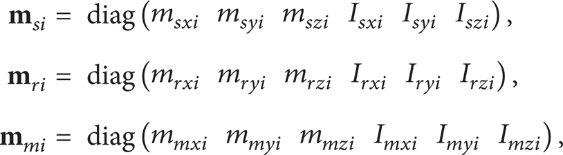
where m _sxi , m _syi , m _szi , I _sxi , I _syi , and I _szi are mass and inertial elements of the spherical joint; m _rxi , m _ryi , m _rzi , I _rxi , I _ryi , and I _rzi are mass and inertial elements of the revolute joint; m _mxi , m _myi , m _mzi , I _mxi , I _myi , and I _mzi are mass and inertial elements of the servomotor.

The formulation of (23) can also be expressed as

$\left(-{\omega }^{\mathrm{2}}{\mathbf{M}}_i+{\mathbf{K}}_{fi}\right){\mathbf{U}}_i={\mathbf{F}}_i,$

(26)

where K _fi = iω C _i + K _i .

3.3. Dynamic Model of Moving Platform

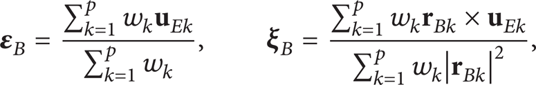
As shown in Figure 6, the equations of motion of the moving platform can be formulated by using the free body diagram as follows:

$\begin{array}{c}{\mathbf{m}}_P{\ddot{\mathbf{\epsilon }}}_P=-{\displaystyle \sum }_{i=\mathrm{1}}^{\mathrm{3}}{\mathbf{F}}_{PLi}+{\mathbf{F}}_P,\\ {\mathbf{I}}_P{\ddot{\mathbf{\xi }}}_P=-{\displaystyle \sum }_{i=\mathrm{1}}^{\mathrm{3}}{\mathbf{r}}_{A_i}\times {\mathbf{F}}_{PLi}+{\mathit{\tau }}_P,\end{array}$

(27)

where m _P and I _P are mass and inertial matrices of the moving platform measured in B − x _B y _B z _B ; ε _P and ξ _P are the linear and angular general coordinates of the moving platform; F _PLi is the reaction force vector at the interface between the moving platform and the ith limb; r _Ai is the vector pointing from the mass center of moving platform to the center of spherical joint; F _P and τ _P are external forces and moments acting on the moving platform, respectively. And we have

${\mathbf{m}}_P=\mathbf{R}{\mathbf{m}}_{P0}{\mathbf{R}}^{\text{T}},\hspace{1em}\hspace{1em}{\mathbf{I}}_P=\mathbf{R}{\mathbf{I}}_{P0}{\mathbf{R}}^{\text{T}},\hspace{1em}\hspace{1em}{\mathbf{F}}_{PLi}={\mathbf{R}}_i{\mathbf{f}}_{PLi},$

(28)

where m _P0 and I _P0 are the mass and inertia matrices of the moving platform measured in the body fixed coordinate system.

Figure 6:

Force diagram of moving platform.

4. Substructure Synthesis

In this section, the governing dynamical equations of the system are established with the substructure synthesis combining with the compatibility conditions at interface of the substructures. The joint stiffness is deduced based on stiffness equivalence criterion and then used for the deformation compatibility analysis.

4.1. Joint Stiffness

The stiffness of the joint may produce important influence on the system dynamical compliance [29]. To improve the simulation precision of the dynamical characteristics of the PKM, the joint stiffness must be considered delicately in the modeling processing.

4.1.1. Stiffness Modeling of the Revolute Joint Assemblage

The revolute joint connects the limb substructures to the base substructure, which is mainly comprised of the rear bearing of the lead-screw, lead-screw nut, closed frame, ball guideway subassembly, and revolute bearing. As shown in Figures 3 and 5, the revolute joint can be simplified as lumped springs, of which the stiffness coefficient can be deduced by the stiffness matrices of revolute bearing subassembly ${{}^b\mathbf{k}}_{ri}$ , closed frame ${}^f{\mathbf{k}}_{ri}$ , ball guideway subassembly ${{}^g\mathbf{k}}_{ri}$ , and lead-screw subassembly ${{}^c\mathbf{k}}_{ri}$ . Herein, the stiffness coefficient of revolute bearing subassembly about x _i is zero, and the others are evaluated by the bearings handbook and the installation conditions. The stiffness matrix of closed frame is constant and can be evaluated using finite element method. The diagonal matrices of revolute bearing subassembly and closed frame can be expressed as

$\begin{array}{c}{{}^b\mathbf{k}}_{ri}=\mathrm{diag}\left(\begin{array}{cccccc}{{}^{b}k}_{r\mathrm{1}xi}& {{}^{b}k}_{r\mathrm{1}yi}& {{}^{b}k}_{r\mathrm{1}zi}& \mathrm{0}& {{}^{b}k}_{r\mathrm{2}yi}& {{}^{b}k}_{r\mathrm{2}zi}\end{array}\right),\\ {}^f{\mathbf{k}}_{ri}=\mathrm{diag}\left(\begin{array}{cccccc}{{}^{f}k}_{r\mathrm{1}xi}& {{}^{f}k}_{r\mathrm{1}yi}& {{}^{f}k}_{r\mathrm{1}zi}& {{}^{f}k}_{r\mathrm{2}xi}& {{}^{f}k}_{r\mathrm{2}yi}& {{}^{f}k}_{r\mathrm{2}zi}\end{array}\right).\end{array}$

(29)

The limb is held by four slide blocks of the ball guideway subassembly, which are carried by the closed frame internally. The ball guideway subassembly can be treated as six virtual lumped springs, one of which is zero along the axial direction of limb. The other stiffness coefficients can be evaluated based on the stiffness equivalence criterion and the slide block distribution mode. We have

${{}^g\mathbf{k}}_{ri}=\mathrm{diag}\left(\begin{array}{cccccc}{{}^{g}k}_{r\mathrm{1}xi}& {{}^{g}k}_{r\mathrm{1}yi}& \mathrm{0}& {{}^{g}k}_{r\mathrm{2}xi}& {{}^{g}k}_{r\mathrm{2}yi}& {{}^{g}k}_{r\mathrm{2}zi}\end{array}\right).$

(30)

The lead-screw subassembly is comprised of the nut, the lead-screw, and the rear support bearing which are serially connected. The stiffness matrix of the lead-screw subassembly can be expressed as

$\begin{array}{c}{{}^c\mathbf{k}}_{ri}=\mathrm{diag}\left(\begin{array}{cccccc}\mathrm{0}& \mathrm{0}& k_{al}& \mathrm{0}& \mathrm{0}& \mathrm{0}\end{array}\right),\\ k_{al}^{-\mathrm{1}}=\frac{\left(l-l_n-q_i\right)}{\text{EA}+k_{an}^{-\mathrm{1}}+k_{ar}^{-\mathrm{1}}},\end{array}$

(31)

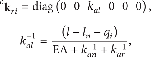
where EA is the tensile modulus of the lead-screw, A = πd_lead²/4, d_lead is the lead-screw diameter, and k _an and k _ar are the stiffness coefficients of the nut and rear support bearing, respectively. After serial and parallel connecting of the subassemblies, the stiffness matrix of the revolute joint can be obtained as

${\mathbf{k}}_{ri}^{-1}={{}^b\mathbf{k}}_{ri}^{-\mathrm{1}}+{{}^f\mathbf{k}}_{ri}^{-\mathrm{1}}+{\left({{}^g\mathbf{k}}_{ri}+{{}^c\mathbf{k}}_{ri}\right)}^{-\mathrm{1}}.$

(32)

Substituting (29)∼(31) into (32), we have

${\mathbf{k}}_{ri}=\mathrm{diag}\left(\begin{array}{cccccc}{k}_{r\mathrm{1}xi}& k_{r\mathrm{1}yi}& k_{r\mathrm{1}zi}& \mathrm{0}& k_{r\mathrm{2}yi}& k_{r\mathrm{2}zi}\end{array}\right),$

(33)

where

$\begin{array}{c}{k}_{r\mathrm{1}xi}={\left({{}^{b}k}_{r\mathrm{1}xi}^{-\mathrm{1}}+{{}^{f}k}_{r\mathrm{1}xi}^{-\mathrm{1}}+{{}^{g}k}_{r\mathrm{1}xi}^{-\mathrm{1}}\right)}^{-\mathrm{1}},\\ k_{r\mathrm{1}yi}={\left({{}^{b}k}_{r\mathrm{1}yi}^{-\mathrm{1}}+{{}^{f}k}_{r\mathrm{1}yi}^{-\mathrm{1}}+{{}^{g}k}_{r\mathrm{1}yi}^{-\mathrm{1}}\right)}^{-\mathrm{1}},\\ k_{r\mathrm{1}zi}={\left({{}^{b}k}_{r\mathrm{1}zi}^{-\mathrm{1}}+{{}^{f}k}_{r\mathrm{1}zi}^{-\mathrm{1}}+k_{al}^{-\mathrm{1}}\right)}^{-\mathrm{1}},\\ k_{r\mathrm{2}yi}={\left({{}^{b}k}_{r\mathrm{2}yi}^{-\mathrm{1}}+{{}^{f}k}_{r\mathrm{2}yi}^{-\mathrm{1}}+{{}^{g}k}_{r\mathrm{2}yi}^{-\mathrm{1}}\right)}^{-\mathrm{1}},\\ k_{r\mathrm{2}zi}={\left({{}^{b}k}_{r\mathrm{2}zi}^{-\mathrm{1}}+{{}^{f}k}_{r\mathrm{2}zi}^{-\mathrm{1}}+{{}^{g}k}_{r\mathrm{2}zi}^{-\mathrm{1}}\right)}^{-\mathrm{1}}.\end{array}$

(34)

4.1.2. Stiffness Modeling of Spherical Joint Assemblage

The spherical joint is used to connect the limb substructures with the moving platform substructure and can be trod as a virtual lumped spring with three orthogonal transverse DOFs. The stiffness matrix of spherical joint can be expressed as

${\mathbf{k}}_{si}=\mathrm{diag}\left(\begin{array}{cccccc}{k}_{sxi}& k_{syi}& k_{syi}& \mathrm{0}& \mathrm{0}& \mathrm{0}\end{array}\right).$

(35)

Note that the spherical joint is a combination of three revolute joints with their axes being orthogonal to one another and the stiffness coefficient k _si varies with the configuration of the PKM. The detailed derivation process was addressed in [3].

4.2. Deformation Compatibility Conditions

As mentioned above, the connection of moving platform with the ith RPS limb can be treated as three virtual transverse lump springs. The displacement relationship between the platform and the limb can be generated as shown in Figure 7. A _iM and A _iL are the interface points associated with the moving platform and RPS limb, respectively. ∇A _i and ε _Ai are displacements of A _iM and A _iL measured in the limb coordinate system B _i − x _i y _i z _i .

Figure 7:

Connection of the spherical joint.

The displacements of the moving platform U _P = (ε _P ,ξ _P )^T and the center of spherical joint A _i have the relationship as follows:

$\begin{array}{c}\nabla {\mathbf{A}}_i={\mathbf{R}}_i^{\mathit{T}}{\mathbf{D}}^{r_{A_i}}{\mathbf{U}}_P,\\ {\mathbf{D}}^{r_{A_i}}=\left[\begin{array}{cccccc}\mathrm{1}& \mathrm{0}& \mathrm{0}& \mathrm{0}& r_{Azi}& -r_{Ayi}\\ \mathrm{0}& \mathrm{1}& \mathrm{0}& -r_{Azi}& \mathrm{0}& r_{Axi}\\ \mathrm{0}& & \mathrm{1}& r_{Ayi}& -r_{Ax{i}_i}& \mathrm{0}\end{array}\right],\end{array}$

(36)

where r _Axi , r _Ayi , and r _Azi are the coordinates of A _i measured in the frame B − x _B y _B z _B .

The reaction forces at the interface between the moving platform and the RPS limb can be expressed as

${\mathbf{f}}_{PLi}=-({\mathbf{k}}_{\mathit{s}i}+i\omega {\mathbf{c}}_{\mathit{s}i})({\mathbf{\epsilon }}_{A_i}-{\mathbf{R}}_i^{\mathit{T}}{\mathbf{D}}^{r_{A_i}}{\mathbf{U}}_P),$

(37)

where c _{s i} = diag⁡(c _sxi , c _syi , c _szi ) is the damping matrix of the spherical joint. Let k _{f s i} = k _{s i} + iωc _{s i} ; the formulation of (37) can be expressed as

${\mathbf{f}}_{PLi}=-{\mathbf{k}}_{f\mathit{s}i}\left({\mathbf{\epsilon }}_{A_i}-{\mathbf{R}}_i^{\mathit{T}}{\mathbf{D}}^{r_{A_i}}{\mathbf{U}}_P\right).$

(38)

Substituting (21) into (38), we have

${\mathbf{f}}_{PLi}=-{\mathbf{k}}_{f\mathit{s}i}\left({\mathbf{N}}_{ci}^{A\mathrm{1}}{\mathbf{u}}_i-{\mathbf{R}}_i^{\mathit{T}}{\mathbf{D}}^{r_{A_i}}{\mathbf{U}}_P\right).$

(39)

Transforming the DOFs u _i measured in B _i − x _i y _i z _i into B − x _B y _B z _B leads to

${\mathbf{f}}_{PLi}=-{\mathbf{k}}_{f\mathit{s}i}\left({\mathbf{N}}_{ci}^{A\mathrm{1}}{\mathbf{T}}_i^{\mathit{T}}{\mathbf{U}}_i-{\mathbf{R}}_i^{\mathit{T}}{\mathbf{D}}^{r_{A_i}}{\mathbf{U}}_P\right).$

(40)

Figure 8 is the diagram of connecting the revolute joint with the base, ${\mathbf{u}}_{B_i}={[{\mathbf{\epsilon }}_{B_i}^{\text{T}}\hspace{1em}{\mathbf{\xi }}_{B_i}^{\text{T}}]}^{\text{T}}$ , and δ _sp are the DOFs of node B _i of the ith limb and the DOFs of base, respectively. We can get the displacement vector as

${\mathit{\delta }}_i=\left[\begin{array}{c}{\mathbf{u}}_{B_i}\\ {\mathit{\delta }}_{sp}\end{array}\right].$

(41)

Figure 8:

Connection of the revolute joint.

The stiffness matrix of connecting the limb with the base is

$\mathbf{k}=\left[\begin{array}{cc}{\mathbf{k}}_{\mathrm{11}}& {\mathbf{k}}_{\mathrm{12}}\\ {\mathbf{k}}_{\mathrm{21}}& {\mathbf{k}}_{\mathrm{22}}\end{array}\right].$

(42)

As the base is fixed, the displacements of the base are zero, ${\mathit{\delta }}_{sp}=\mathbf{0}$ , the stiffness block matrix k₁₁ = diag⁡(k_r1,k_r2), and ${\mathbf{k}}_{\mathrm{12}}={\mathbf{k}}_{\mathrm{21}}={\mathbf{k}}_{\mathrm{22}}=\mathbf{0}$ .

According to the displacement compatibility and the force equilibrium condition, the reaction forces and moments at the interfaces between ith limb and the base can be expressed as

${\mathbf{f}}_{BLi}=-{\mathbf{k}}_{fr\mathrm{1}}{\mathbf{N}}_{ci}^{B\mathrm{1}}{\mathbf{T}}_i^{\mathit{T}}{\mathbf{U}}_i,\hspace{1em}\hspace{1em}{\mathit{\tau }}_{BLi}=-{\mathbf{k}}_{fr\mathrm{2}}{\mathbf{N}}_{ci}^{B\mathrm{2}}{\mathbf{T}}_i^{\mathit{T}}{\mathbf{\xi }}_i,$

(43)

where k_fr1 = k_r1 + iωc_r1, k_fr2 = k_r2 + iωc_r2. c_r1 = diag⁡(c_r1xi, c_r1yi, c_r1zi) and c_r2 = diag⁡(c_r2xi, c_r2yi, c_r2zi) are the linear and angular damping matrices, respectively.

4.3. Dynamic Model of 3-RPS in Global System

Substituting (40) and (43) into (26) and (27), we can obtain the governing equations of motion of the system:

$\mathbf{M}\ddot{\tilde{\mathbf{U}}}+\mathbf{C}\dot{\tilde{\mathbf{U}}}+\mathbf{K}\tilde{\mathbf{U}}=\tilde{\mathbf{F}},$

(44)

where $\tilde{\mathbf{F}}=e^{i\omega t}\mathbf{F}$ , $\tilde{\mathbf{U}}=e^{i\omega t}\mathbf{U}$ . M, C, and K are the global mass, damping, and stiffness matrices, and U and F are the global general coordinates vector and external load vector, respectively.

Let K _f = iωC + K, and (44) can be transformed to

$\left(-{\omega }^{\mathrm{2}}\mathbf{M}+{\mathbf{K}}_f\right)\mathbf{U}=\mathbf{F}.$

(45)

Herein

$\begin{array}{c}\mathbf{M}=\mathrm{diag}\left({\mathbf{M}}_{\mathrm{1}}\mathbf{,}\hspace{0.17em}\hspace{0.17em}{\mathbf{M}}_{\mathrm{2}}\mathbf{,}\hspace{0.17em}\hspace{0.17em}{\mathbf{M}}_{\mathrm{3}}\mathbf{,}\hspace{0.17em}\hspace{0.17em}{\mathbf{M}}_{\mathrm{4}}\right),\\ {\mathbf{M}}_{\mathrm{4}}=\mathrm{diag}\left({\mathbf{m}}_P,{\mathbf{I}}_P\right),\\ \mathbf{U}=\left\{\begin{array}{c}{\mathbf{U}}_{\mathrm{1}}\\ {\mathbf{U}}_{\mathrm{2}}\\ {\mathbf{U}}_{\mathrm{3}}\\ {\mathbf{U}}_{\mathrm{4}}\end{array}\right\},\hspace{1em}\hspace{1em}{\mathbf{U}}_{\mathrm{4}}=\left\{\begin{array}{c}{\mathbf{\epsilon }}_P\\ {\mathbf{\xi }}_P\end{array}\right\},\\ \mathbf{F}=\left\{\begin{array}{c}{\mathbf{F}}_{\mathrm{1}}\\ {\mathbf{F}}_{\mathrm{2}}\\ {\mathbf{F}}_{\mathrm{3}}\\ {\mathbf{F}}_{\mathrm{4}}\end{array}\right\},\hspace{1em}\hspace{1em}{\mathbf{F}}_{\mathrm{4}}=\left\{\begin{array}{c}{\mathbf{F}}_P\\ {\mathit{\tau }}_P\end{array}\right\},\\ {\mathbf{K}}_f=\left[\begin{array}{cccc}{\mathbf{K}}_{f\mathrm{1,1}}& & & {\mathbf{K}}_{f\mathrm{1,4}}\\ & {\mathbf{K}}_{f\mathrm{2,2}}& & {\mathbf{K}}_{f\mathrm{2,4}}\\ & & {\mathbf{K}}_{f\mathrm{3,3}}& {\mathbf{K}}_{f\mathrm{3,4}}\\ {\mathbf{K}}_{f\mathrm{4,1}}& {\mathbf{K}}_{f\mathrm{4,2}}& {\mathbf{K}}_{f\mathrm{4,3}}& {\mathbf{K}}_{f\mathrm{4,4}}\end{array}\right],\\ {\mathbf{K}}_{fi,i}={\left({\mathbf{N}}_{ci}^{A\mathrm{1}}\right)}^{\mathit{T}}{\mathbf{R}}_i{\mathbf{k}}_{fsi}{\mathbf{R}}_i^{\mathit{T}}{\mathbf{N}}_{ci}^{A\mathrm{1}}+{\left({\mathbf{N}}_{ci}^{B\mathrm{1}}\right)}^{\mathit{T}}{\mathbf{R}}_i{\mathbf{k}}_{fr\mathrm{1}}{\mathbf{R}}_i^{\mathit{T}}{\mathbf{N}}_{ci}^{B\mathrm{1}}\hspace{1em}+{\left({\mathbf{N}}_{ci}^{B\mathrm{2}}\right)}^{\mathit{T}}{\mathbf{R}}_i{\mathbf{k}}_{fr\mathrm{2}}{\mathbf{R}}_i^{\mathit{T}}{\mathbf{N}}_{ci}^{B\mathrm{2}}+{\mathbf{K}}_{fi},\\ {\mathbf{K}}_{f\mathrm{4,4}}=\left[\begin{array}{c}{\displaystyle \sum }_{i=\mathrm{1}}^{\mathrm{3}}{\mathbf{R}}_i{\mathbf{k}}_{fsi}{\mathbf{R}}_i^{\mathit{T}}{\mathbf{D}}^{r_{A_i}}\\ {\displaystyle \sum }_{i=\mathrm{1}}^{\mathrm{3}}{\mathbf{r}}_{A_i}\times \left({\mathbf{R}}_i{\mathbf{k}}_{fsi}{\mathbf{R}}_i^{\mathit{T}}{\mathbf{D}}^{r_{A_i}}\right)\end{array}\right],\\ {\mathbf{K}}_{fi,\mathrm{4}}=-{\left({\mathbf{N}}_{ci}^{A\mathrm{1}}\right)}^{\text{T}}{\mathbf{R}}_i{\mathbf{k}}_{fsi}{\mathbf{R}}_i^{\mathit{T}}{\mathbf{D}}^{r_{A_i}},\\ {\mathbf{K}}_{f\mathrm{4},i}=\left[\begin{array}{c}-{\mathit{R}}_i{\mathbf{k}}_{fsi}{\mathbf{R}}_i^{\mathit{T}}{\mathbf{N}}_{ci}^{A\mathrm{1}}\\ -{\mathbf{r}}_{A_i}\times {\mathbf{R}}_i{\mathbf{k}}_{fsi}{\mathbf{R}}_i^{\mathit{T}}{\mathbf{N}}_{ci}^{A\mathrm{1}}\end{array}\right].\end{array}$

(46)

5. Dynamic Characteristics Prediction and Validation

In this section, dynamic characteristics analysis of a prototype of the A3 head shown in Figure 1 is carried out to illustrate the effectiveness of the above-proposed method. The geometrical parameters of the A3 head are listed in Table 1. Herein, p _z = s + d is the distance between center point of moving platform and center point of base, s = 0∼200 is the stroke along the axes z, and θ_max is the maximal posture angle. The position when s = 0 is defined as the initial position of the A3 head.

Table 1:

The geometrical parameters of the A3 head (unit: mm).

a	b	s	d	l	l n	θmax (°)	d lead
250	250	0∼200	550	1150	125	± 40	23.5

5.1. Natural Frequency of the 3-RPS

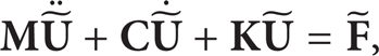
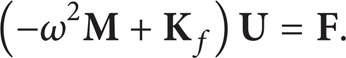
In this section, the eigenvalue and eigenvector evaluation is conducted to predict the distributions of lower natural frequencies of the A3 head throughout the entire workspace. Neglecting the influence of the damping, the equation of the free vibration of the system can be obtained from (45) as

$\left(\mathbf{K}-{\omega }^{\mathrm{2}}\mathbf{M}\right)\mathbf{U}=\mathrm{0}.$

(47)

The characteristic equation of (47) is

$\left|\mathbf{K}-{\omega }^{\mathrm{2}}\mathbf{M}\right|=\mathrm{0}.$

(48)

By solving (48), we can get the kth (k = 1, 2,…, n) eigenvalue ω _k ² and eigenvector U _k . Herein, ω _k and U _k are the kth natural frequency and modal shape of the system, and the global modal coordinates can be expressed as

$\mathbf{U}=\left[\begin{array}{cccc}{\mathbf{U}}_{\mathrm{1}}& {\mathbf{U}}_{\mathrm{2}}& \cdots & {\mathbf{U}}_n\end{array}\right].$

(49)

Figure 9 shows the distributions of lower natural frequencies of A3 head over the working plane of P _z = 550 mm. It can be found that the first six orders of natural frequencies of the A3 head are axisymmetric over the given work plane. This is coincident with the axial symmetry of the structure of three RPS limbs in the PKM. It also indicates that the distributions of the lower natural frequencies of the A3 head are strongly configuration-related. Herein, the first-order natural frequency decreases from the maximal value of 29.5 Hz at θ = 0° to the minimal value of 16 Hz at θ = 40°. The second-order natural frequency varies from the minimal value of 29.6 Hz to the maximal value of 34.6 Hz. The intervals of the third- to sixth-order natural frequencies are [49.2∼42.8] Hz, [49.3∼51.79] Hz, [57.2∼64.07] Hz, and [73.01∼66.05] Hz, respectively. It should be indicated that the values of the first- and second-order natural frequencies are close to each other at the orientation of θ = 0° and separated when the orientation angle increased.

Figure 9:

Natural frequencies’ distributions over the working plane at p _z = 550 mm.

5.2. Natural Frequency and Mode Shapes Validation of the 3-RPS

In this subsection, the natural frequencies, modal shapes, and dynamic responses at the end of the moving platform are measured to validate the correctness of proposed dynamical modeling method. Figure 10 is the experimental test rig to measure the dynamical characteristics of the A3 head at the position of P _z = 550 mm and the orientation of θ _x = θ _y = 0°. The testing rig includes a data acquisition system and an LMS modal testing system in which modal analysis and FRF curve fitting were carried out. The LMS front is SC-305 with 8 input/output channels. Accelerometers are piezoelectricity accelerating sensor produced by B&K Company and used to pick up the responses. The impact hammer is PCB086C03 with the force sensor installed internally and the sensitivity is 11.9 mV/N. Sampling frequency is set as 1024 Hz and the sampling time is set as 2 s. Frequency resolution is set as 0.5 Hz. The window function is force exponential with 50% force window and 10% exponential window. Each measuring run is the averaged result of five impacts. During the process of modal test, the excitation point is fixed at the end of the moving platform while the pickup points of dynamical response are changing correspondingly [30]. The FRFs from exciting points to recording points can be calculated, and homologous elements of transfer function in arbitrary row or column can be obtained. Then, with the technique of modal identification and fitness, the natural frequencies, modal shapes, damping ratios, and the FRFs of the system can be obtained. The detailed experimental method of the A3 head was addressed in our previous work in [31].

Figure 10:

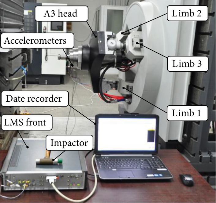
Experimental setup to measure the dynamical characteristics.

Figure 11 is the wire-frame diagram comparison of the first five orders of modal shapes between analytical and experimental models. The corresponding natural frequency values as well as the prediction errors of analytic and experiment at the initial position are listed in Table 2. It can be found that the errors of the first three orders of natural frequencies are small, and the maximum was less than 5%. The errors of fourth and fifth orders of natural frequencies are relatively larger, and the maximum was up to 13.5%.

Table 2:

The natural frequencies of the 3-RPS (unit: Hz).

ω n	1st mode	2nd mode	3rd mode	4th mode	5th mode
Analytic	29.5	29.6	49.2	49.3	57.2
Experiment	29.2	30	49.4	57.4	65.4
Error (%)	1.2	1.4	0.4	14.1	12.5

Figure 11:

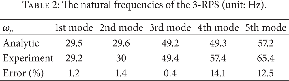
Comparison of natural frequencies and mode shapes between the analytic and experimental methods.

It can be found from Figure 11 that the first order of modal shape is reciprocating vibration of the whole system along y-axes, in which all limbs oscillate up and down; the second order of modal shape is reciprocating vibration of the whole system along x-axes, in which all limbs swing horizontally; the third order of modal shape is external and internal reciprocating vibration of the limbs, bending about the y _i -axes with respect to the limb reference frame B _i − x _i y _i z _i , with limb1 stretching forward and back along its axis besides its bending. It should also be pointed out that the first two orders of modal shapes obtained by the proposed method coincide well with the experimental ones. The predicted vibrations of limb2 and limb3 in third order of modal shape are in agreement with the experimental ones. And the predicted vibration mode of limb 1 is agreed upon to test results only with an opposite vibration phase.

Figures 11(g) to 11(j) show that the fourth-order modal shape is the vibrations of limb 2 and limb 3 about y _i -axes with respect to the limb frame B _i − x _i y _i z _i in the opposite way, and the fifth-order modal shape is the vibrations of limb 1 to limb 3 about y _i -axes in the same way. The vibrations of limb 2 and limb 3 in the fourth and fifth orders of modal shapes in the analytical model coincide with the experimental ones. However, the predicting accuracy of limb 1 is relatively less. It can be found in Figures 11(g) and 11(h) that the experimental vibration of limb 1 which vibrates about both x _i and y _i is more complex than the analytical one. The vibration of the limb 1 in the fifth order of modal shape only vibrates about y _i -axes; however, the corresponding one also combined with the vibration about x _i .

It can be found from the comparison of the analytical and experimental values that the differences between theoretical calculation and experimental testing results of the fourth and fifth orders are a little bit more than those of lower orders. The main reason for this phenomenon is that the spherical and revolute joints in the theoretical model are treated as ideal ones with the same pretightening force and stiffness coefficients. However, the preloads and assembling errors of the joints in the actual prototype are different because of the manufacturing errors, leading to the differences of the stiffness coefficients of the spherical and revolute joints in each limb assembly. The stiffness errors of the joints result in the prediction errors of the whole system in the further dynamical characteristic analysis. The comparisons of the simulated and experimental modal shapes indicate that the preloads of spherical and revolute joints of limb 1 assembly should be improved. It can be seen from the modal shape diagrams that the vibration magnitude of the bodies is relatively slight compared with the vibration magnitudes of the joints. Therefore, great effort should be made to ensure the joint rigidities.

5.3. Frequency Response Analysis of the 3-RPS

In this subsection, the position-dependent dynamic response of the A3 head is analyzed using the dynamical modeling method proposed in this paper. The system mass and stiffness matrices in (44) can be transferred to the end of the moving platform as follows:

$\begin{array}{c}{\mathbf{M}}_{\mathbf{t}}={\mathbf{T}}_{\text{T}}^{\mathit{\text{'}}}{\mathbf{T}}_A^{\mathit{\text{'}}}\mathbf{M}{\left({\mathbf{T}}_A^{\text{T}}\right)}^{\prime }{\left({\mathbf{T}}_{\text{T}}^{\text{T}}\right)}^{\prime },\\ {\mathbf{K}}_{\mathbf{t}}={\mathbf{T}}_{\text{T}}^{\mathit{\text{'}}}{\mathbf{T}}_A^{\mathit{\text{'}}}\mathbf{K}{\left({\mathbf{T}}_A^{\text{T}}\right)}^{\prime }{\left({\mathbf{T}}_{\text{T}}^{\text{T}}\right)}^{\prime },\end{array}$

(50)

where M _t and K _t are the system mass and stiffness matrices with respect to the reference frame A _t − uvw, T _A is the transformation matrices from the frame B − x _B y _B z _B to the frame A − uvw, and T_T is the transformation matrices from the frame A − uvw to the frame A _t − uvw and can be expressed as

${\mathbf{T}}_{\text{T}}=\left[\begin{array}{cc}\mathbf{R}& \mathrm{0}\\ {\widehat{\mathbf{w}}}_t\mathbf{R}& \mathbf{R}\end{array}\right],\hspace{1em}\hspace{1em}{\mathbf{T}}_A=\left[\begin{array}{cc}\mathit{I}& \mathrm{0}\\ {\widehat{\mathbf{r}}}_A& \mathit{I}\end{array}\right],$

(51)

where the superscript “ $\widehat{\hspace{0.5em}}$ ” denotes the skew-symmetric transformation; thus,

${\widehat{\mathbf{w}}}_t=\left[\begin{array}{ccc}\mathrm{0}& -w_{tz}& \mathrm{0}\\ w_{tz}& \mathrm{0}& \mathrm{0}\\ \mathrm{0}& \mathrm{0}& \mathrm{0}\end{array}\right],\hspace{1em}\hspace{1em}{\widehat{\mathbf{r}}}_A=\left[\begin{array}{ccc}\mathrm{0}& -r_{Az}& r_{Ay}\\ r_{Az}& \mathrm{0}& -r_{Ax}\\ -r_{Ay}& r_{Ax}& \mathrm{0}\end{array}\right],$

(52)

where ${\mathbf{w}}_t={\left[\begin{array}{ccc}\mathrm{0}& \mathrm{0}& w_{tz}\end{array}\right]}^{\text{T}}$ is the position vector of the endpoint of moving platform with respect to the frame A − uvw and w _tz is the distance from the endpoint to the center point of the moving platform.

Experiment shows that the A3 head prototype is a complex modal system. To simplify the damping problem in modeling [21], we assume that the system has structural damping (resulting from the joint friction) proportional to the system stiffness matrix and (44) becomes

${\mathbf{M}}_{\mathbf{t}}\ddot{\tilde{\mathbf{U}}}+\left(\mathrm{1}+j\eta \right){\mathbf{K}}_{\mathbf{t}}\tilde{\mathbf{U}}=\tilde{\mathbf{F}},$

(53)

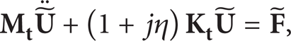
where η is the damping factor. Thus, the displacement FRFs for the system can be written as

${\mathbf{H}}_d\left(\omega \right)=\mathbf{\Phi }\left[\mathrm{diag}\frac{\mathrm{1}}{m_i({\omega }_i^{\mathrm{2}}-\omega +j\eta {\omega }_i^{\mathrm{2}})}\right]{\mathbf{\Phi }}^{\text{T}},$

(54)

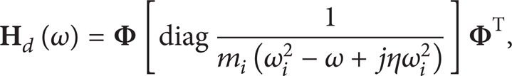
where Φ is the system eigenvector matrix, which can be proved for proportional damping system to be the same as in the undamping system. m _i = Φ _i ^TM _t Φ _i is the modal mass. The damping factor η can be obtained by the empirical equation based on the tested damping values at the initial position.

Figure 12 displays the comparison of the original real and imaginary parts of FRFs between the simulation and the experiment along the u direction with respect to the frame A − uvw at the initial position. In the figure, black solid curves stand for the FRFs obtained by the experimental method and the red dashed curves are calculated by the theoretical method proposed. Apparently, there exists a good agreement at resonant peaks of interest. It can be found that the natural frequency of the highest peak of the tested FRF is about 29 Hz, and a lower peak happens in the frequency value about 70 Hz. The imaginary parts of FRFs play a main role in the dynamical response of the system, of which the maximal magnitude is 1.2 × 10⁻⁶ m/N, while the corresponding real parts of FRFs are 7 × 10⁻⁷ m/N.

Figure 12:

FRF comparisons between measured and analytic methods.

The mode with maximal peak of the FRF is defined as major modal, which influences the dynamic behavior of the system dramatically. The simulation shows that the first two order modes are two dense natural frequencies, no matter at what configuration the A3 head is set, and two repeated natural frequencies when the structure is completely symmetric. It has also been approved by the natural frequencies distributions in Figure 9. These characteristics of the PKMs can also be found in [20, 21].

Figure 12 displays the comparison of FRF curves along u-axes obtained by the measured method, analytic and FE model at the position of P _z = 750 mm, and the orientation of θ _x = θ _y = 0°. The real and imaginary FRFs in Figure 12 show that the simulation precision of the low order resonant peaks of FRFs using the analytical method is higher than the corresponding ones of the high order modes, which have been fully approved in the previous natural frequencies and modal shapes analysis. It can be also found that there is a small peak in the analytical FRFs and the corresponding natural frequency is about 60 Hz, while the corresponding natural frequency in the measured FRFs is about 70 Hz. Thus, the natural frequencies of the high order modes obtained by the proposed method are smaller than the corresponding one measured. The full order flexible FE model of the A3 head is also established using the same joint stiffness coefficients to simulation of the dynamical response, and the blue dash-dotted curves shown in Figure 12 are simulated in ANSYS environment. It is obviously shown that the FRF curves obtained by the FE model coincide well with the measured FRF curves at the small resonant peak of the high order mode. However, the simulation precision of FE model at the resonant peak of the major modal is less than the analytical method. The corresponding natural frequencies of the major modal are higher than the measured ones.

Figure 13 shows the comparison of the analytical and measured distributions of the amplitude FRFs varying with the configurations of A3 head. The diagrams on the left are obtained by the analytical method, and the right ones are measured by the LMS system. It can be found in these figures that the original FRFs at the end of moving platform are strongly position-dependent, and the maximal dynamical compliance arises when the PKM is complete trisymmetrical. Figures 13(a) and 13(c) display the distributions of calculated FRFs in the direction of u-axes and v-axes of the body fixed frame A − uvw, respectively, when the orientation angle θ _y varies from − 30° to 30° about y-axes at the position of P _z = 750 mm and the orientation of θ _x = 0°. It can be seen that the dynamic compliance distributions are symmetric, and the maximum value appears at θ _x = θ _y = 0°. With the increasing of absolute value of orientation angle θ _y , dynamic compliances of the major modal along u-axes and v-axes both decrease, and the values of magnitude along u-axes decrease obviously. It should also be indicated that the major modals at the initial orientation are repeated natural frequencies of the first two order modes and separate into two dense natural frequencies when the absolute value of θ _y increases. This phenomenon can also be found in the distributions of the natural frequencies.

Figure 13:

The FRFs distributions at P _z = 750 mm, θ _x = 0°, and θ _y = − 30°∼30°.

Figures 14(a) and 14(c) show the distributions of calculated FRFs along u-axes and v-axes of the frame A − uvw, respectively, when the orientation angle θ _y = 0° and θ _x varies from − 30° to 30° about x-axes over the work plane P _z = 750 mm. It can be seen from Figure 14(a) that the natural frequencies of the major modal along u-axes increase when θ _x varies from − 30° to 30°, while the variations of the magnitude values are slight. Figure 14(c) shows that the maximum value of dynamic compliance along v-axis appears at the orientation of θ _x = − 5° and θ _y = 0°, and the dynamic compliances of the major modal decrease, no matter with the increase or decrease of θ _x . The distributions of measured FRFs in Figures 14(b) and 14(d) express the same variation tendencies as shown by the calculated ones using analytical method proposed.

Figure 14:

The FRFs distributions at P _z = 750 mm, θ _y = 0°, and θ _x = − 30°∼30°.

It can be seen from the distributions of FRFs in Figures 13 and 14 that the magnitude of the dynamic compliance decreases if the orientation angular θ increases, and the corresponding dynamic stiffness will increase accordingly, which is helpful to improve the chatter stability of the A3 head based high-speed machining [32].

6. Conclusions

This paper presents a computationally efficient elastodynamic model for a fully flexible 3-RPS PKM. Comparing with the traditional full orders FE model, the distributions of the dynamical characteristics of the PKM can be rapidly evaluated at any desired configuration in this semianalytical model. The simulated natural frequencies, modal shapes, and dynamical responses are validated by the experiment tests. The major conclusions can be drawn as follows.

1. Based on the substructure synthesis and modal reduction technique, a semianalytical dynamic model is established. With the proposed model, the distributions of the natural frequencies and FRFs throughout the entire workspace can be predicted in a quick manner.

2. The distributions of the natural frequencies and FRFs of the A3 head indicate that the dynamic characteristics of the system are strongly position-dependent and axially symmetric due to its kinematic and structural features.

3. The simulation accuracies of lower orders of the natural frequencies are higher than those of higher orders ones, relatively. The maximal predicting errors are less than 15% at the initial position.

4. It can be seen from the first five modal shapes that the vibration magnitudes of the joints are higher than the other bodies, indicating that great effort should be made to ensure the joint rigidities.

5. The highest resonant peaks of the dynamic compliance appear at the natural frequencies of the first two orders of modes, and the maximal dynamic compliance arises when the PKM is completely trisymmetrical.

6. The major modes at the initial orientation are repeated natural frequencies of the first two order modes and separate into two dense natural frequencies when the orientation angle increases.

7. The good agreement between the simulation and the experiment of the dynamic characteristics indicates the effectiveness of the modeling method. With the rapid evaluation for the dynamic responses, a further detailed investigation associated with high-speed machining stability will be carried out and reported in separate articles.

Conflict of Interests

The authors declare that there is no conflict of interests regarding the publication of this paper.