Development of Discrete Adjoint Approach Based on the Lattice Boltzmann Method

Abstract

The purpose of this research is to present a general procedure with low implementation cost to develop the discrete adjoint approach for solving optimization problems based on the LB method. Initially, the macroscopic and microscopic discrete adjoint equations and the cost function gradient vector are derived mathematically, in detail, using the discrete LB equation. Meanwhile, for an elementary case, the analytical evaluation of the macroscopic and microscopic adjoint variables and the cost function gradients are presented. The investigation of the derivation procedure shows that the simplicity of the Boltzmann equation, as an alternative for the Navier-Stokes (NS) equations, can facilitate the process of extracting the discrete adjoint equation. Therefore, the implementation of the discrete adjoint equation based on the LB method needs fewer attempts than that of the NS equations. Finally, this approach is validated for the sample test case, and the results gained from the macroscopic and microscopic discrete adjoint equations are compared in an inverse optimization problem. The results show that the convergence rate of the optimization algorithm using both equations is identical and the evaluated gradients have a very good agreement with each other.

1. Introduction

The adjoint method is one of the gradient-based techniques in which gradient vector of the cost function with respect to design variables is calculated indirectly by solving an adjoint equation. Although an additional cost arises from solving the adjoint equation, the gradients of the cost function can be altogether achieved with respect to each design variable. Consequently, the total cost to obtain these gradients is independent of the number of design variables and amounts to the cost of two flow solutions roughly [1]. Therefore, these methods are widely used for the gradient computation when the problem contains numerous design variables [2]. Adjoint methods solve a large class of optimization, inverse, and control problems [3–8]. Another important application is posterior error estimation. In this context, these methods are often called duality based methods [9, 10] which are particularly useful when the original problem is a discretized partial differential equation. When the numerical error caused by the discretization is high, the automatic adaptive mesh refinement [11] based on the adjoint solution can be applied to reduce the numerical error at a fixed computational cost. There are two approaches to develop the adjoint equation: continuous and discrete. Continuous adjoint approach utilizes the differential forms of the governing equations of the flow field and cost function. But, in the discrete adjoint approach, the adjoint equation is directly extracted from a set of discrete flow field equations and the cost function is gained from a numerical approximation of the equations. The importance of the discrete version is that the exact gradient of the discrete cost function is obtained [12]. This ensures that the optimization process can converge fully. Moreover, creation of the adjoint program is conceptually straightforward. This benefit includes the iterative solution process since the transposed matrix has the same eigenvalues as the original linear matrix, and so the same iterative solution method is guaranteed to converge [5]. But, a major disadvantage of this version is the complexity of the adjoint equation derived from the discrete flow field (Navier-Stokes) equations, so that the complete extraction of all the discrete terms in the adjoint equation and the gradient vector requires a lot of algebraic manipulations. In addition, the viscous flux in the NS equations further increases the complexity of deriving the terms in viscous flows. The discrete adjoint equation becomes very complicated when the flow field (NS) equations are discretized with higher order schemes and using flux limiters [2]. Therefore the implementation cost of the discrete adjoint equation based on the NS equations is usually higher in comparison with the LB-based equation.

In comparison with the conventional flow field (NS) equations, the LB method uses the Boltzmann transport equation to solve the flow field. Due to the lower complexity of the LB equation, the implementation of this method would be considerably easier. The importance of this benefit will become more clear when a gradient-based technique is used in optimization problems involving flow field equations (irrespective of the flow field solution) in optimization process. The simplicity of the Boltzmann equation, as an alternative to the conventional flow field equations, can be very helpful in facilitating the process of extracting the continuous adjoint equation (and particularly the discrete adjoint equation). Moreover, the LB method uses an inherently immersed boundary grid system. This unique feature of the LB method enables the modeling of complicated geometries and the analysis of flows around them in a straightforward manner without the need for conventional body-fitted grid generation. So, by exploiting the LB method, the optimization of special geometries is done with lower cost [13]. Furthermore, it can remove the drawbacks of nongradient techniques, which necessitate a lot of flow solutions (due to the selective random design variables) and consequently the application of grid generation. Additionally, in gradient methods, there is no need to consider some grid modification techniques. Besides, the inherent parallel processing nature of the LB method, owing to data transfer from the nearest neighbor in terms of streaming and fully localized calculations of collision phase, distinguishes it from the conventional methods of computational fluid dynamics [14]. This capability of the LB method seems to be very effective in the analysis of complex unsteady flows [15, 16] and optimization problems with a large number of design variables or constraints that demand long computational times [13, 14]. As a result, it is possible to employ some optimization techniques which are not efficient for traditional computational fluid dynamics due to the high computational cost (e.g., adjoint method in problems with high number of constraints or nongradient methods in problems with high number of design variables). Taking into account all the aforementioned advantages, the significance of flow optimization utilizing the LB method becomes obvious compared to the other conventional techniques. These unique advantages of the LB method form the main idea of its application to optimization problems.

Execution of the adjoint optimization approach by means of conventional NS-based computational methods has been extensively studied in recent decades, for instance, through the works of Jameson [8, 17, 18], Elliot and Peraire [19], Nadarajah [2, 12], Hekmat et al. [20, 21], Tonomura et al. [22], Jacques and Dwight [23], Hicken and Zingg [24], and Freund [25]. However, there are few researches in combination with the adjoint method and the LB method. Tekitek et al. [26], for the first time, performed the discrete adjoint approach via the LB method. They extracted the discrete adjoint equation based on the LB equation to identify the unknown parameters of the LB method without representing a general framework and evaluating the details of the adjoint variables and gradients. In addition, Pingen et al. [14, 27] explored the ability of the incompressible LB method in topology optimization problems. Their major work was focused on the extraction of steady discrete adjoint equation and gradient of cost function using the steady LB equation and its implicit solution. Moreover, they examined the performance of mathematical algorithms (e.g., iterative and direct algorithms) to solve these equations implicitly. Their research was restricted to optimization in steady flows and did not offer an overall framework for implementation and computation.

In this research, for the first time, both macroscopic and microscopic discrete adjoint equations are extracted based on the LB method using a general procedure with low implementation cost. The proposed approach can be performed similarly for any optimization problem with the corresponding cost function and design variables vector. Moreover, this approach is not limited to flow fields and can be employed for steady as well as unsteady flows. The main focus is to derive the macroscopic and microscopic discrete adjoint equations using the LB method. The validity of this development is examined for an unsteady laminar poiseuille flow in an infinite periodic channel with uniform and constant body forces, using an inverse optimization problem. Moreover, the accuracy of the cost function gradients is evaluated by comparison to the results of the finite difference approach.

2. Lattice Boltzmann Method

2.1. Lattice Boltzmann Equation

For a system without an external force, the Boltzmann-BGK equation can be written as

$\frac{\partial f}{\partial t}+c·\nabla f=\frac{\mathrm{1}}{\lambda }\left(f^{\text{eq}}-f\right),$

(1)

where f = f(x, c, t) is the density distribution function, c is the particle velocity vector, t is time, and the dot (·) denotes the scalar product. Here, the local equilibrium distribution function is denoted by f^eq and λ is called the relaxation time. In the LB method, (1) is discretized in velocity or phase space and assumed to be valid along specific directions. Hence, the discrete Boltzmann equation can be written along i direction as

$\frac{\partial f_i}{\partial t}+c_i·\nabla f_i=\frac{\mathrm{1}}{\lambda }\left(f_i^{\text{eq}}-f_i\right),$

(2)

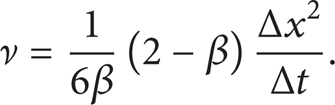
where f _i is the distribution function along i direction and f _i ^eq is the corresponding local equilibrium distribution function. The left-hand side of the above equation represents the streaming or propagation process, where the distribution function streams along the lattice link i with velocity c _i = Δx/Δt (Δx and Δt are the displacement and time steps, resp.) and the right-hand side represents the rate of change of the distribution function in the collision process. Equation (2) is now discretized with respect to space and time, using a first-order upwind finite difference approximation in time and space, resulting in the discretized LB equation:

$f_i\left(x+c_i\Delta t,t+\Delta t\right)=\left(\mathrm{1}-\beta \right)f_i\left(x,t\right)+\beta f_i^{\text{eq}}\left(x,t\right),$

(3)

where β = Δt/λ is the inverse of the dimensionless relaxation time. To facilitate the implementation of the LB method, it is common to choose time step Δt and lattice spacing Δx equal to 1 (c = 1).

In an incompressible flow, ideally, so that the divergence of the velocity is zero, the density is assumed to be equal to the initial density; that is, ρ = ρ₀. Therefore, assuming an order O(Ma²) density fluctuation, the equilibrium distribution function is obtained using Taylor series expansion of the Maxwell-Boltzmann equilibrium distribution and ignoring O(Ma³) terms or higher [28, 29]:

$f_i^{\text{eq}}=\rho w_i{\Theta }_i,\hspace{1em}{\Theta }_i=\mathrm{1}+\frac{\mathrm{3}\left(c_i·u\right)}{c^{\mathrm{2}}}+\frac{\mathrm{9}{\left(c_i·u\right)}^{\mathrm{2}}}{\mathrm{2}{c}^{\mathrm{4}}}-\frac{\mathrm{3}{u}^{\mathrm{2}}}{\mathrm{2}{c}^{\mathrm{2}}},$

(4)

where u≡u(x, t) and ρ≡ρ(x, t) are the macroscopic velocity vector and density, respectively. Also, w _i is the lattice weight parameter in i direction that depends on the lattice arrangement.

2.2. D2Q9 Model

In this study, the two-dimensional, nine-velocity D2Q9 lattice model is used (see Figure 1).

Figure 1:

Lattice arrangement of the D2Q9 model.

These velocity vectors $c_i={[c_{i,x},c_{i,y}]}^T$ can be written as

$c_i=\{\begin{array}{cc}\left(\mathrm{0,0}\right)\hfill & i=\mathrm{0}\hfill \\ (\cos \left[\frac{\left(i-\mathrm{1}\right)\pi }{\mathrm{2}}\right],\hfill & \hfill \\ \phantom{lll}\sin \left[\frac{\left(i-\mathrm{1}\right)\pi }{\mathrm{2}}\right])c\hfill & i=\mathrm{1,2},\mathrm{3,4}\hfill \\ \sqrt{\mathrm{2}}(\cos \left[\frac{\left(i-\mathrm{5}\right)\pi }{\mathrm{2}}+\frac{\pi }{\mathrm{4}}\right],\hfill & \hfill \\ \phantom{llllllll}\sin \left[\frac{\left(i-\mathrm{5}\right)\pi }{\mathrm{2}}+\frac{\pi }{\mathrm{4}}\right])c\hfill & i=\mathrm{5,6},\mathrm{7,8}.\hfill \end{array}$

(5)

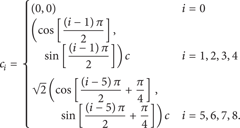
For the D2Q9 model, the lattice weight parameters are as [28]

$w_i=\{\begin{array}{cc}\frac{4}{9}\hfill & i=\mathrm{0}\hfill \\ \frac{1}{9}\hfill & i=\mathrm{1,2},\mathrm{3,4}\hfill \\ \frac{1}{36}\hfill & i=\mathrm{5,6},\mathrm{7,8}.\hfill \end{array}$

(6)

For low Mach number (Ma ≪ 1) or low density fluctuation (Δρ/ρ ≪ 1) flows, it is possible to recover the macroscopic incompressible NS equations from the LB equation using the Chapman-Enskog expansion and choosing the kinematic viscosity as [27]

$\nu =\frac{\mathrm{1}}{\mathrm{6}\beta }\left(\mathrm{2}-\beta \right)\frac{\Delta x^{\mathrm{2}}}{\Delta t}.$

(7)

Also, the macroscopic properties such as density ρ and velocity vector $u={[u^x,u^y]}^T$ in lattice units can be evaluated by taking statistical moments of the distribution function, leading to the following equations:

$\rho ={{\displaystyle \sum }}_{i=\mathrm{0}}^{\mathrm{8}}{f}_i\left(x,t\right),\hspace{1em}\hspace{1em}u=\frac{\mathrm{1}}{{\rho }_{\mathrm{0}}}{{\displaystyle \sum }}_{i=\mathrm{0}}^{\mathrm{8}}{c}_i{f}_i\left(x,t\right).$

(8)

Furthermore, the speed of sound (c _s ) is $c/\sqrt{\mathrm{3}}$ for the D2Q9 model [29].

3. General Description of the Discrete Adjoint Method

Consider a general flow field. The properties which define the cost function I are functions of the state variables θ and the design variables, which may be represented by the function κ:

$I=I\left(\theta ,\kappa \right).$

(9)

Since the state variables depend on the design variables, θ = θ(κ), a variation in κ changes θ and finally these variations result in a change:

$\delta I={\left[\frac{\partial I}{\partial \theta }\right]}_I^T\delta \theta +{\left[\frac{\partial I}{\partial \kappa }\right]}_{II}^T\delta \kappa .$

(10)

Here, the subscripts I and II are used to distinguish the contributions due to δθ from δκ in the cost function variation δI. In fact, changes in the design variables either directly or indirectly can lead to changes in the cost function. The first term is the indirect effect of the design variables on the cost function that appears as the change in the state variables, and the second term is the direct effect of the design variables on the cost function. Suppose that the governing equation R which expresses the dependence of θ and κ within the flow field domain can be written as

$R(\theta ,\kappa )=\mathrm{0}.$

(11)

In fact, the governing equation of the flow field is the correlation between the state and the design variables (the state and the design variables are only correlated by the governing equation of the flow field). Therefore, δθ can be determined as

$\delta R={\left[\frac{\partial R}{\partial \theta }\right]}_I^{}\delta \theta +{\left[\frac{\partial R}{\partial \kappa }\right]}_{II}^{}\delta \kappa =\mathrm{0}.$

(12)

Since variation δR is zero, it can be multiplied by a Lagrange multiplier (adjoint variable) ψ and subtracted from the variation δR with no change in the result. Thus, (10) can be replaced by

$\begin{array}{c}\delta I={\left[\frac{\partial I}{\partial \theta }\right]}^T\delta \theta +{\left[\frac{\partial I}{\partial \kappa }\right]}^T\delta F-{\psi }^T\left(\left[\frac{\partial R}{\partial \theta }\right]\delta \theta +\left[\frac{\partial R}{\partial \kappa }\right]\delta F\right)\\ \hspace{1em}={\left\{{\left[\frac{\partial I}{\partial \theta }\right]}^T-{\psi }^T\left[\frac{\partial R}{\partial \theta }\right]\right\}}_I\delta \theta +{\left\{{\left[\frac{\partial I}{\partial \kappa }\right]}^T-{\psi }^T\left[\frac{\partial R}{\partial \kappa }\right]\right\}}_{II}\delta F.\end{array}$

(13)

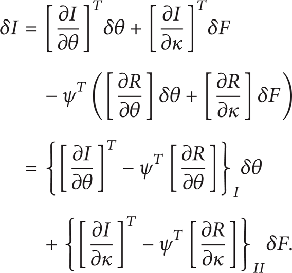
Now, the adjoint variable ψ is determined such that the dependency of the cost function variation on the state variables variation is eliminated. Therefore, choosing ψ to satisfy the adjoint equation

${\left[\frac{\partial R}{\partial \theta }\right]}^T\psi =\frac{\partial I}{\partial \theta },$

(14)

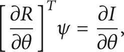
the first term is eliminated, and we find that

$\delta I=G\delta \kappa ,$

(15)

where the cost function gradient G with respect to the design variable κ is obtained by

$G={\left[\frac{\partial I}{\partial \kappa }\right]}^T-{\psi }^T\left[\frac{\partial R}{\partial \kappa }\right].$

(16)

According to (15) and (16), δI is independent of δθ and, as a result, for a large number of design variables, we can compute the cost function gradient only with one flow solution in addition to one adjoint solution in each optimization cycle. In fact, the computational cost of the adjoint equation solution is independent of the number of the design variables.

4. Optimization Problem Statement

On the whole, an optimization problem in an unsteady flow can be expressed in the following general form:

$\begin{array}{l}\underset{{\theta }_t\in R^m,\kappa \in R^n}{\mathrm{Min}}I\left({\theta }_t,\kappa \right)\\ \text{s}.\text{t}.R_t\left({\theta }_t,\kappa \right)=\mathrm{0},\hspace{1em}t\in \Lambda ,\end{array}$

(17)

where θ _t is the m-dimensional state variables vector at time t, κ is the n-dimensional design variables vector, R _t is the governing equation of the flow field, and I is the value of cost function at the time interval of Λ≡[0, t _f ] that can be written in the general form as

$I\left({\theta }_t,\kappa \right)={{\displaystyle \int }}_{\Lambda }{I}_t\left({\theta }_t,\kappa \right)dt={{\displaystyle \int }}_{\Lambda }{{\displaystyle \int }}_{\Gamma }{I}_{tx}\left({\theta }_t,\kappa \right)dx\hspace{0.17em}dt,$

(18)

wherein I _t is the cost function at time t and Γ is the flow field domain. Using numerical integration rule and supposing that Δx = Δt = 1, the cost function (18) can be evaluated as

$I\left({\theta }_t,\kappa \right)={{\displaystyle \sum }}_{t=\mathrm{0}}^{t_f}{I}_t\left({\theta }_t,\kappa \right)={{\displaystyle \sum }}_{t=\mathrm{0}}^{t_f}{{\displaystyle \sum }}_x{I}_{tx}\left({\theta }_t,\kappa \right),$

(19)

where ∑ _x ‍ is performed over all the lattice points of Γ.

4.1. Cost Function

The inverse problem is employed in this study to validate the adjoint equation, the gradient vector acquired from the LB method, and the applied optimization algorithm. Therefore, the target flow field is selected using the target design variables. Subsequently, assuming unknown values for the target design variables, it is favorable to find the optimal design variables that lead to the target flow field. Hence, the local cost function at time t can be described as

$I_{tx}=\frac{\mathrm{1}}{\mathrm{2}}{\left|w_t-w_t^d\right|}^{\mathrm{2}}+\frac{\sigma }{\mathrm{2}}{\left|\kappa \right|}^{\mathrm{2}},$

(20)

where $w_t={[{\rho }_t,u_t^x,u_t^y]}^T\in R^{\mathrm{3}}$ is the flow field variables (macroscopic properties) vector at time t and w _t ^d is the desired flow field variables vector at time t. The first term in the cost function measures the distance of w _t and w _t ^d and the second term is a regularization term with σ ≥ 0 (typically, σ ∈ [10e − 5, 10e − 3]), which leads to improved smoothness properties of the optimization problem for σ > 0 [30].

4.2. Design Variables

In this investigation, the external body forces vector applied to the fluid is regarded as the design variables vector. Thus, the expression

$V_i=c_s^{\mathrm{2}}(c_i·\kappa )$

(21)

is added to the right-hand side of (2). In the above equation, $\kappa ={[{\kappa }^x,{\kappa }^y]}^T\in R^2$ is the 2D body forces (design variables) vector. Therefore, considering the force term (21), the LB equation (3) can be rewritten in the following vector form:

$F_{t+\mathrm{1}}=\left(\mathrm{1}-\beta \right)F_t+\beta F_t^{\text{eq}}+V,$

(22)

where $F_t\equiv F(x,t)={[f_{0,t},\dots ,f_{8,t}]}^T\in R^9$ is the distribution functions (microscopic properties) vector at time t and $V={[V_0,\dots ,V_8]}^T$ . It can be shown that the existence of the force term (21) in the LB equation results in the recovery of the NS equations in the presence of the body force κ [31].

5. Discrete Adjoint Approach Based on the Lattice Boltzmann Method

In this section, the macroscopic and microscopic discrete adjoint equations and the cost function gradient vector are mathematically derived using the discrete LB equation. Also, for the present test case, the analytical evaluation of the macroscopic and microscopic adjoint variables and the cost function gradients are presented.

5.1. Derivation of the Macroscopic Discrete Adjoint Equation

In the optimization problem (17), the design variables variation, in the path towards the optimal values, must be such that the governing equation of the flow field is always satisfied at any point of space and at any time. Therefore, the flow field governing equation is considered as a constraint for the optimization problem. Here, the conservation equations (8) and the flow field variables (macroscopic properties) vector w _t are chosen as the constraint and the state variables vector θ _t in the optimization problem, respectively. The conservation equations (8) can be rewritten in the following vector form:

$w_t={\Phi }_t\left(w_{t-\mathrm{1}},\kappa \right),\hspace{1em}t=\mathrm{1},\dots ,t_f.$

(23)

For ρ₀ = 1,

${\Phi }_t\left(w_{t-\mathrm{1}},\kappa \right)=\left[\begin{array}{c}{\Phi }_t^{\mathrm{1}}\left(w_{t-\mathrm{1}},\kappa \right)\\ {\Phi }_t^{\mathrm{2}}\left(w_{t-\mathrm{1}},\kappa \right)\\ {\Phi }_t^{\mathrm{3}}\left(w_{t-\mathrm{1}},\kappa \right)\end{array}\right]=\left[\begin{array}{c}{\displaystyle \sum }_{i=\mathrm{0}}^{\mathrm{8}}{f}_i\\ {\displaystyle \sum }_{i=\mathrm{0}}^{\mathrm{8}}{c}_{ix}{f}_i\\ {\displaystyle \sum }_{i=\mathrm{0}}^{\mathrm{8}}{c}_{iy}{f}_i\end{array}\right].$

(24)

Remark 1. According to (22), it can be deduced that the distribution functions f _i at time t are functions of the flow field variables in previous time step, w_{t − 1}, and the design variables κ.

Finally, the constraint R _t in the problem (17) based on the LB method can be expressed as

$R_t\left(w_t,\kappa \right)=w_t-{\Phi }_t\left(w_{t-\mathrm{1}},\kappa \right)=\mathrm{0},\hspace{1em}t=\mathrm{1},\dots ,t_f.$

(25)

The optimization problem is now treated as a control problem where the design variables vector κ represents the control function, which is chosen to minimize the cost function (19) subjected to the constraint of satisfaction of the flow field governing equation (25) at any time, any point of the lattice space, and any direction of the lattice lines.

Since the flow field variables vector depends on the design variables vector implicitly, w _t = w _t (κ), a variation δκ in the design variables vector causes a variation δw _t in the flow field variables vector, and consequently, these variations lead to a variation δI in the cost function (19):

$\begin{array}{l}\delta I={{\displaystyle \sum }}_{t=\mathrm{0}}^{t_f}{{\displaystyle \sum }}_x^{}\delta I_{tx}\left(w_t,\kappa \right)\\ \hspace{0.17em}={{\displaystyle \sum }}_{t=\mathrm{1}}^{t_f}{{\displaystyle \sum }}_x^{}\left[{\frac{\partial I_{tx}}{\partial w_t}}^T\left(w_t,\kappa \right)\delta w_t+{\frac{\partial I_{tx}}{\partial \kappa }}^T\left(w_t,\kappa \right)\delta \kappa \right].\end{array}$

(26)

It should be noted that, with considering constant value for initial conditions of the LB equation, in the optimization process, variation of the flow field and the design variables vector at t = 0 are zero. Also, the variation in the flow field variables vector due to the variation in the design variables vector is such that the conservation equations (25) will be always satisfied. Hence, we have

$\begin{array}{l}\delta R_t\left(w_t,\kappa \right)=\delta w_t-\delta {\Phi }_t\left(w_{t-\mathrm{1}},\kappa \right)\\ \hspace{1em}\hspace{1em}\hspace{0.17em}=\delta w_t-\frac{\partial {\Phi }_t}{\partial w_{t-\mathrm{1}}}\left(w_{t-\mathrm{1}},\kappa \right)\delta w_{t-\mathrm{1}}-\frac{\partial {\Phi }_t}{\partial \kappa }\left(w_{t-\mathrm{1}},\kappa \right)\delta \kappa \\ \hspace{1em}\hspace{1em}\hspace{0.17em}=\mathrm{0},\hspace{1em}t=\mathrm{1},\dots ,t_f.\end{array}$

(27)

Now, multiplying the adjoint variables vector ${\psi }_t\equiv \psi (x,t)={[{\psi }_t^1,{\psi }_t^2,{\psi }_t^3]}^T\in R^{\mathrm{3}}$ by (27)

${\psi }_t^T\delta R_t={\psi }_t^T\delta w_t-{\psi }_t^T\frac{\partial {\Phi }_t}{\partial w_{t-\mathrm{1}}}\delta w_{t-\mathrm{1}}-{\psi }_t^T\frac{\partial {\Phi }_t}{\partial \kappa }\delta \kappa =\mathrm{0},\hspace{1em}t=\mathrm{1},\dots ,t_f,$

(28)

and then summing over the time and space and considering δw _t = 0 and δκ = 0 at t = 0, we get

${{\displaystyle \sum }}_{t=\mathrm{1}}^{t_f}{{\displaystyle \sum }}_x^{}{\psi }_t^T\delta R_t={{\displaystyle \sum }}_{t=\mathrm{1}}^{t_f}{{\displaystyle \sum }}_x^{}\left[{\psi }_t^T\delta w_t-{\psi }_t^T\frac{\partial {\Phi }_t}{\partial \kappa }\delta \kappa \right]-{{\displaystyle \sum }}_{t=\mathrm{2}}^{t_f}{{\displaystyle \sum }}_x^{}{\psi }_t^T\frac{\partial {\Phi }_t}{\partial w_{t-\mathrm{1}}}\delta w_{t-\mathrm{1}}=\mathrm{0}.$

(29)

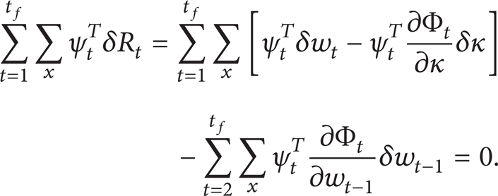
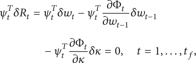
Equation (29) can be subtracted from the variation (26) with no change in the result to give

$\begin{array}{l}\delta I={{\displaystyle \sum }}_{t=\mathrm{1}}^{t_f}{{\displaystyle \sum }}_x^{}\left[{\frac{\partial I_{tx}}{\partial w_t}}^T\delta w_t+{\frac{\partial I_{tx}}{\partial \kappa }}^T\delta \kappa \right]-{{\displaystyle \sum }}_{t=\mathrm{1}}^{t_f}{{\displaystyle \sum }}_x^{}\left[{\psi }_t^T\delta w_t-{\psi }_t^T\frac{\partial {\Phi }_t}{\partial \kappa }\delta \kappa \right]+{{\displaystyle \sum }}_{t=\mathrm{2}}^{t_f}{{\displaystyle \sum }}_x^{}{\psi }_t^T\frac{\partial {\Phi }_t}{\partial w_{t-\mathrm{1}}}\delta w_{t-\mathrm{1}}\\ \hspace{0.17em}={\displaystyle \sum }_x[\left\{{{\displaystyle \sum }}_{t=\mathrm{1}}^{t_f}\left({\frac{\partial I_{tx}}{\partial w_t}}^T-{\psi }_t^T\right)\delta w_t+{{\displaystyle \sum }}_{t=\mathrm{2}}^{t_f}{\psi }_t^T\frac{\partial {\Phi }_t}{\partial w_{t-\mathrm{1}}}\delta w_{t-\mathrm{1}}\right\}+\left\{{{\displaystyle \sum }}_{t=\mathrm{1}}^{t_f}\left({\frac{\partial I_{tx}}{\partial \kappa }}^T+{\psi }_t^T\frac{\partial {\Phi }_t}{\partial \kappa }\right)\delta \kappa \right\}].\end{array}$

(30)

The first term on the last line of the equation can be rewritten as

$\begin{array}{l}{{\displaystyle \sum }}_{t=\mathrm{1}}^{t_f}\left({\frac{\partial I_{tx}}{\partial w_t}}^T-{\psi }_t^T\right)\delta w_t+{{\displaystyle \sum }}_{t=\mathrm{2}}^{t_f}{\psi }_t^T\frac{\partial {\Phi }_t}{\partial w_{t-\mathrm{1}}}\delta w_{t-\mathrm{1}}\\ \hspace{0.17em}={{\displaystyle \sum }}_{t=\mathrm{1}}^{t_f}\left({\frac{\partial I_{tx}}{\partial w_t}}^T-{\psi }_t^T\right)\delta w_t+{{\displaystyle \sum }}_{t=\mathrm{1}}^{t_f-\mathrm{1}}{\psi }_{t+\mathrm{1}}^T\frac{\partial {\Phi }_{t+\mathrm{1}}}{\partial w_t}\delta w_t\\ \hspace{0.17em}=\left({\frac{\partial I_{t_{f}x}}{\partial w_{t_f}}}^T-{\psi }_{t_f}^T\right)\delta w_{t_f}+{{\displaystyle \sum }}_{t=\mathrm{1}}^{t_f-\mathrm{1}}\left({\frac{\partial I_{tx}}{\partial w_t}}^T-{\psi }_t^T+{\psi }_{t+\mathrm{1}}^T\frac{\partial {\Phi }_{t+\mathrm{1}}}{\partial w_t}\right)\delta w_t.\end{array}$

(31)

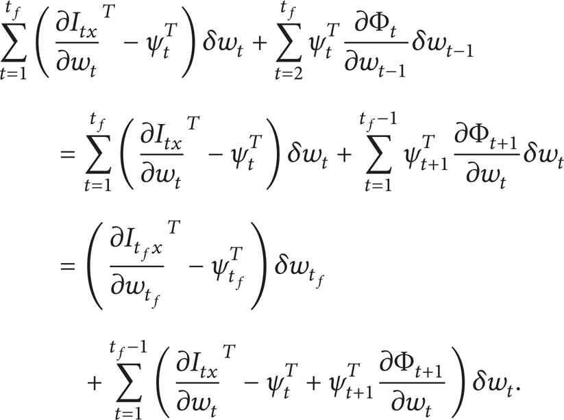
Substituting (31) into (30), we have

$\delta I={\displaystyle \sum }_x[{\left\{{\frac{\partial I_{t_{f}x}}{\partial w_{t_f}}}^T-{\psi }_{t_f}^T\right\}}_I\delta w_{t_f}+{{\displaystyle \sum }}_{t=\mathrm{1}}^{t_f-\mathrm{1}}{\left\{{\frac{\partial I_{tx}}{\partial w_t}}^T-{\psi }_t^T+{\psi }_{t+\mathrm{1}}^T\frac{\partial {\Phi }_{t+\mathrm{1}}}{\partial w_t}\right\}}_I\delta w_t]+{{\displaystyle \sum }}_x{{\displaystyle \sum }}_{t=\mathrm{1}}^{t_f}{\left\{{\frac{\partial I_{tx}}{\partial \kappa }}^T+{\psi }_t^T\frac{\partial {\Phi }_t}{\partial \kappa }\right\}}_{II}\delta \kappa .$

(32)

Now, the adjoint variables vector ψ _t is chosen such that the changes of the cost function δI are independent from the changes of the flow field variables vector δw _t . As a result, by setting the first and second terms on the right-hand side of the equation equal to zero, the terminal adjoint condition

${\psi }_{t_f}=\frac{\partial I_{t_{f}x}}{\partial w_{t_f}}$

(33)

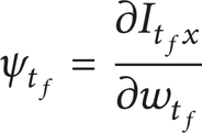
and the unsteady discrete adjoint equation

${\psi }_t^T={\frac{\partial I_{tx}}{\partial w_t}}^T+{\psi }_{t+\mathrm{1}}^T\frac{\partial {\Phi }_{t+\mathrm{1}}}{\partial w_t},\hspace{1em}t=t_f-\mathrm{1},\dots ,\mathrm{1}$

(34)

are attained, respectively.

Remark 2. It should be noted that the adjoint variables ψ _t ¹, ψ _t ², and ψ _t ³ correspond to the flow field variables (macroscopic properties) ρ _t , u _t ^x , and u _t ^y . Therefore, ψ _t ¹ to ψ _t ³ can be referred to as the macroscopic adjoint variables and (34) can be called the macroscopic discrete adjoint (MADA) equation. Note that the present derivatives in the MADA equation are evaluated with respect to the macroscopic properties vector w _t .

The macroscopic adjoint variables vector ψ _t is obtained by solving the MADA equation together with the adjoint terminal condition such that the variation of the cost function δI is independent from the variation of the flow field variables vector δw _t . Thus, by eliminating the terms on the first line of (32), we have

$\delta I={{\displaystyle \sum }}_x{{\displaystyle \sum }}_{t=\mathrm{1}}^{t_f}\left\{{\frac{\partial I_{tx}}{\partial \kappa }}^T+{\psi }_t^T\frac{\partial {\Phi }_t}{\partial \kappa }\right\}\delta \kappa .$

(35)

Finally, the gradient vector G will be obtained by

$G={\nabla }_{\kappa }I={{\displaystyle \sum }}_x{{\displaystyle \sum }}_{t=\mathrm{1}}^{t_f}\left\{{\frac{\partial I_{tx}}{\partial \kappa }}^T+{\psi }_t^T\frac{\partial {\Phi }_t}{\partial \kappa }\right\}.$

(36)

Also,

$G_t={\nabla }_{\kappa }{I}_t={{\displaystyle \sum }}_x\left\{{\frac{\partial I_{tx}}{\partial \kappa }}^T+{\psi }_t^T\frac{\partial {\Phi }_t}{\partial \kappa }\right\},\hspace{1em}t=\mathrm{1},\dots ,t_f,$

(37)

where G _t is the cost function gradient vector with respect to the design variables vector at time t.

Remark 3. Comparing the discrete LB equation with the MADA equation, it is observed that, as was expected, the MADA equation is quite similar to the discrete LB equation and this equation has the inherent aspects of the original LB equation (e.g., linearity, simplicity, etc.). Therefore, it is expected that the computational cost for solving this equation is nearly equal to that of the LB equation. The main difference between these equations is in their solving procedure. In the LB method, the flow field variables vector is evaluated by solving the discrete LB equation at time interval [1, t _f ] as forward in time, while, in the adjoint method, the macroscopic adjoint variables vector is evaluated by solving the MADA equation at the same interval as backward in time. Figure 2 shows the evaluating procedure of the adjoint variables as backward in time using the evaluated flow field variables as forward in time.

Figure 2:

The flow field variables evaluated and collected as forward in time and used later for evaluating the macroscopic adjoint variables as backward in time.

5.1.1. Evaluation of the Macroscopic Adjoint Variables Vector

To evaluate the macroscopic adjoint variables vector using the MADA equation, first, the derivatives ∂I _tx /∂w _t and ∂Φ_{t + 1}/∂w _t should be evaluated. Considering the cost function (20), we have

$\frac{\partial I_{tx}}{\partial w_t}={\left[\begin{array}{ccc}\frac{\partial I_{tx}}{\partial {\rho }_t}& \frac{\partial I_{tx}}{\partial u_t^x}& \frac{\partial I_{tx}}{\partial u_t^y}\end{array}\right]}^T=\left[\begin{array}{c}{\rho }_t-{\rho }_t^d\\ u_t^x-u_t^{x,d}\\ u_t^y-u_t^{y,d}\end{array}\right].$

(38)

The evaluation of the derivative Φ_{t + 1} with respect to w _t using the LB equation requires further investigation. First, it is appropriate to write the derivative ∂Φ_{t + 1}/∂w _t in a matrix form as

$\frac{\partial {\Phi }_{t+\mathrm{1}}}{\partial w_t}=\left[\begin{array}{ccc}\frac{\partial {\Phi }_{t+\mathrm{1}}^{\mathrm{1}}}{\partial {\rho }_t}& \frac{\partial {\Phi }_{t+\mathrm{1}}^{\mathrm{1}}}{\partial u_t^x}& \frac{\partial {\Phi }_{t+\mathrm{1}}^{\mathrm{1}}}{\partial u_t^y}\\ \frac{\partial {\Phi }_{t+\mathrm{1}}^{\mathrm{2}}}{\partial {\rho }_t}& \frac{\partial {\Phi }_{t+\mathrm{1}}^{\mathrm{2}}}{\partial u_t^x}& \frac{\partial {\Phi }_{t+\mathrm{1}}^{\mathrm{2}}}{\partial u_t^y}\\ \frac{\partial {\Phi }_{t+\mathrm{1}}^{\mathrm{3}}}{\partial {\rho }_t}& \frac{\partial {\Phi }_{t+\mathrm{1}}^{\mathrm{3}}}{\partial u_t^x}& \frac{\partial {\Phi }_{t+\mathrm{1}}^{\mathrm{3}}}{\partial u_t^y}\end{array}\right].$

(39)

For example, consider the first array of the above matrix (∂Φ_{t + 1}¹/∂ρ _t ). According to (23) and (24), we have

$\begin{array}{c}\frac{\partial {\Phi }_{t+\mathrm{1}}^{\mathrm{1}}}{\partial {\rho }_t}=\frac{\partial {\rho }_{t+\mathrm{1}}}{\partial {\rho }_t}=\frac{\partial }{\partial {\rho }_t}\left[{{\displaystyle \sum }}_{i=\mathrm{0}}^{\mathrm{8}}{f}_i\right]\hfill \\ \hspace{0.17em}=\frac{\partial }{\partial {\rho }_t}{f}_{\mathrm{0}}(x_{i,j},t+\mathrm{1})+\frac{\partial }{\partial {\rho }_t}{f}_{\mathrm{1}}(x_{i,j},t+\mathrm{1})+\cdots +\frac{\partial }{\partial {\rho }_t}{f}_{\mathrm{7}}\left(x_{i,j},t+\mathrm{1}\right)+\frac{\partial }{\partial {\rho }_t}{f}_{\mathrm{8}}\left(x_{i,j},t+\mathrm{1}\right),\end{array}$

(40)

where x _{i, j} ≡(x _i , y _j ) is the spatial discretized form of the location vector x for the lattice node (i, j)th. To evaluate the derivative of the distribution functions f₀ to f₈ with respect to density ρ _t , first, the distribution functions at time t + 1 must be expressed as functions of density ρ _t explicitly. Here, we have little hesitation and return to the LB equation. Consider a k × l lattice (k and l are the number of lattice nodes along the horizontal and the vertical axis, resp.) in a rectangular solution domain with flow inlet and outlet boundaries at i = 1 and i = k, respectively, and solid walls at j = 1 and i = l. Expanding of the LB equation (22) for each lattice node (i, j), we have

$\begin{array}{c}{f}_{\mathrm{0}}\left(x_{i,j},t+\mathrm{1}\right)=\left(\mathrm{1}-\beta \right)f_{\mathrm{0}}\left(x_{i,j},t\right){+\beta f_{\mathrm{0}}^{\text{eq}}\left(x_{i,j},t\right)|}_{i=\mathrm{1},\dots ,k,j=\mathrm{1},\dots ,l},\\ f_{\mathrm{1}}\left(x_{i,j},t+\mathrm{1}\right)=(\mathrm{1}-\beta )f_{\mathrm{1}}(x_{i-\mathrm{1},j},t){+\beta f_{\mathrm{1}}^{\text{eq}}\left(x_{i-\mathrm{1},j},t\right)+c_s^{\mathrm{2}}{\kappa }^x|}_{i=\mathrm{2},\dots ,k,j=\mathrm{1},\dots ,l},\\ ⋮\\ f_{\mathrm{7}}\left(x_{i,j},t+\mathrm{1}\right)=(\mathrm{1}-\beta )f_{\mathrm{7}}(x_{i+\mathrm{1},j+\mathrm{1}},t)+\beta f_{\mathrm{7}}^{\text{eq}}(x_{i+\mathrm{1},j+\mathrm{1}},t){\mathrm{\hspace{0.17em}\hspace{0.17em}}-c_s^{\mathrm{2}}\left({\kappa }^x+{\kappa }^y\right)|}_{i=\mathrm{1},\dots ,k-\mathrm{1},j=\mathrm{1},\dots ,l-\mathrm{1}},\\ f_{\mathrm{8}}\left(x_{i,j},t+\mathrm{1}\right)=(\mathrm{1}-\beta )f_{\mathrm{8}}(x_{i-\mathrm{1},j+\mathrm{1}},t)+\beta f_{\mathrm{8}}^{\text{eq}}(x_{i-\mathrm{1},j+\mathrm{1}},t){+c_s^{\mathrm{2}}\left({\kappa }^x-{\kappa }^y\right)|}_{i=\mathrm{2},\dots ,k,j=\mathrm{1},\dots ,l-\mathrm{1}}.\end{array}$

(41)

The other not-computed distribution functions are computed by applying the periodic boundary condition at the inlet boundary as

$\begin{array}{l}{f}_{\mathrm{1}}\left(x_{\mathrm{1},j},t+\mathrm{1}\right)=(\mathrm{1}-\beta )f_{\mathrm{1}}(x_{k,j},t){+\beta f_{\mathrm{1}}^{\text{eq}}\left(x_{k,j},t\right)+c_s^{\mathrm{2}}{\kappa }^x|}_{j=\mathrm{1},\dots ,l},\\ f_{\mathrm{5}}\left(x_{\mathrm{1},j},t+\mathrm{1}\right)=(\mathrm{1}-\beta )f_{\mathrm{5}}(x_{k,j-\mathrm{1}},t){+\beta f_{\mathrm{5}}^{\text{eq}}\left(x_{k,j-\mathrm{1}},t\right)++c_s^{\mathrm{2}}\left({\kappa }^x+{\kappa }^y\right)|}_{j=\mathrm{2},\dots ,l},\\ f_{\mathrm{8}}\left(x_{\mathrm{1},j},t+\mathrm{1}\right)=(\mathrm{1}-\beta )f_{\mathrm{8}}(x_{k,j+\mathrm{1}},t){+\beta f_{\mathrm{8}}^{\text{eq}}(x_{k,j+\mathrm{1}},t)+c_s^{\mathrm{2}}({\kappa }^x-{\kappa }^y)|}_{j=\mathrm{1},\dots ,l-\mathrm{1}}\end{array}$

(42)

and at the outlet boundary as

$\begin{array}{l}{f}_{\mathrm{3}}\left(x_{k,j},t+\mathrm{1}\right)=\left(\mathrm{1}-\beta \right)f_{\mathrm{3}}\left(x_{\mathrm{1},j},t\right){+\beta f_{\mathrm{3}}^{\text{eq}}\left(x_{\mathrm{1},j},t\right)-c_s^{\mathrm{2}}{\kappa }^x|}_{j=\mathrm{1},\dots ,l},\\ f_{\mathrm{6}}\left(x_{k,j},t+\mathrm{1}\right)=\left(\mathrm{1}-\beta \right)f_{\mathrm{6}}\left(x_{\mathrm{1},j-\mathrm{1}},t\right){+\beta f_{\mathrm{6}}^{\text{eq}}\left(x_{\mathrm{1},j-\mathrm{1}},t\right)-c_s^{\mathrm{2}}\left({\kappa }^x-{\kappa }^y\right)|}_{j=\mathrm{2},\dots ,l},\\ f_{\mathrm{7}}\left(x_{k,j},t+\mathrm{1}\right)=\left(\mathrm{1}-\beta \right)f_{\mathrm{7}}\left(x_{\mathrm{1},j+\mathrm{1}},t\right){+\beta f_{\mathrm{7}}^{\text{eq}}\left(x_{\mathrm{1},j+\mathrm{1}},t\right)-c_s^{\mathrm{2}}\left({\kappa }^x+{\kappa }^y\right)|}_{j=\mathrm{1},\dots ,l-\mathrm{1}}\end{array}$

(43)

and applying the no-sleep boundary condition by the complete bounce-back scheme at the lower solid wall

$\begin{array}{l}{f}_{\mathrm{2}}\left(x_{i,\mathrm{1}},t+\mathrm{1}\right)=\left(\mathrm{1}-\beta \right)f_{\mathrm{4}}\left(x_{i,\mathrm{1}},t\right){+\beta f_{\mathrm{4}}^{\text{eq}}\left(x_{i,\mathrm{1}},t\right)-c_s^{\mathrm{2}}{\kappa }^y|}_{i=\mathrm{1},\dots ,k},\\ f_{\mathrm{5}}\left(x_{i,\mathrm{1}},t+\mathrm{1}\right)=(\mathrm{1}-\beta )f_{\mathrm{7}}(x_{i,\mathrm{1}},t){+\beta f_{\mathrm{7}}^{\text{eq}}\left(x_{i,\mathrm{1}},t\right)-c_s^{\mathrm{2}}\left({\kappa }^x+{\kappa }^y\right)|}_{i=\mathrm{1},\dots ,k},\\ f_{\mathrm{6}}\left(x_{i,\mathrm{1}},t+\mathrm{1}\right)=(\mathrm{1}-\beta )f_{\mathrm{8}}(x_{i,\mathrm{1}},t){+\beta f_{\mathrm{8}}^{\text{eq}}(x_{i,\mathrm{1}},t)+c_s^{\mathrm{2}}({\kappa }^x-{\kappa }^y)|}_{i=\mathrm{1},\dots ,k}\end{array}$

(44)

and the upper solid wall

$\begin{array}{l}{f}_{\mathrm{4}}\left(x_{i,l},t+\mathrm{1}\right)=(\mathrm{1}-\beta )f_{\mathrm{2}}(x_{i,l},t){+\beta f_{\mathrm{2}}^{\text{eq}}\left(x_{i,l},t\right)+c_s^{\mathrm{2}}{\kappa }^y|}_{i=\mathrm{1},\dots ,k},\\ f_{\mathrm{7}}\left(x_{i,l},t+\mathrm{1}\right)=(\mathrm{1}-\beta )f_{\mathrm{5}}(x_{i,l},t){+\beta f_{\mathrm{5}}^{\text{eq}}\left(x_{i,l},t\right)+c_s^{\mathrm{2}}\left({\kappa }^x+{\kappa }^y\right)|}_{i=\mathrm{1},\dots ,k},\\ f_{\mathrm{8}}\left(x_{i,l},t+\mathrm{1}\right)=(\mathrm{1}-\beta )f_{\mathrm{6}}(x_{i,l},t){+\beta f_{\mathrm{6}}^{\text{eq}}\left(x_{i,l},t\right)-c_s^{\mathrm{2}}\left({\kappa }^x-{\kappa }^y\right)|}_{i=\mathrm{1},\dots ,k}.\end{array}$

(45)

In the terms on the right-hand side of (41) to (45), only the equilibrium distribution functions are functions of the flow field variables vector. Therefore, with considering the equilibrium distribution function (4), all the distribution functions at time t + 1 can be rewritten in terms of the flow field variables at time t. Now, we return to (40). For example, it is possible to evaluate ∂f₈/∂ρ _t for all lattice nodes by substituting (4) into (41), (42), and (45) and then taking the derivative of both sides of the obtained equations with respect to ρ _t :

$\begin{array}{l}\frac{\partial f_{\mathrm{8}}}{\partial {\rho }_t}\left(x_{i,j},t+\mathrm{1}\right)=\beta \frac{\partial }{\partial {\rho }_t}{f}_{\mathrm{8}}^{\text{eq}}(x_{i-\mathrm{1},j+\mathrm{1}},t){=\beta w_{\mathrm{8}}{\Theta }_{\mathrm{8}}\left(x_{i-\mathrm{1},j+\mathrm{1}},t\right)|}_{i=\mathrm{2},\dots ,k,j=\mathrm{1},\dots ,l-\mathrm{1}},\\ \frac{\partial f_{\mathrm{8}}}{\partial {\rho }_t}\left(x_{\mathrm{1},j},t+\mathrm{1}\right)=\beta \frac{\partial }{\partial {\rho }_t}{f}_{\mathrm{8}}^{\text{eq}}(x_{k,j+\mathrm{1}},t){=\beta w_{\mathrm{8}}{\Theta }_{\mathrm{8}}\left(x_{k,j+\mathrm{1}},t\right)|}_{j=\mathrm{1},\dots ,l-\mathrm{1}},\\ \frac{\partial f_{\mathrm{8}}}{\partial {\rho }_t}\left(x_{i,l},t+\mathrm{1}\right)=\beta \frac{\partial }{\partial {\rho }_t}{f}_{\mathrm{6}}^{\text{eq}}(x_{i,l},t){=\beta w_{\mathrm{6}}{\Theta }_{\mathrm{6}}\left(x_{i,l},t\right)|}_{i=\mathrm{1},\dots ,k}.\end{array}$

(46)

So, the derivative of the distribution function of f₈ with respect to ρ _t for all the lattice nodes is obtained. Evaluation of the derivative of other distribution functions with respect to ρ _t can be performed in a similar manner. With determination of the derivative of the distribution functions f₀ to f₈ with respect to ρ _t , derivative ∂Φ_{t + 1}¹/∂ρ _t can be fully evaluated. Performing the above process, it is possible to evaluate other arrays of matrix Φ_{t + 1}/∂w _t .

5.1.2. Evaluation of the Gradient Vector

After evaluating the present derivatives in the MADA equation, the macroscopic adjoint variables vector is eventually achieved. Now, to evaluate the gradient vector using (36), first, the derivatives ∂I _tx /∂κ and ∂Φ _t /∂κ should be evaluated. Considering the cost function (20), we have

$\frac{\partial I_{tx}}{\partial \kappa }={\left[\begin{array}{cc}\frac{\partial I_{tx}}{\partial {\kappa }^x}& \frac{\partial I_{tx}}{\partial {\kappa }^y}\end{array}\right]}^T=\sigma \left[\begin{array}{c}{\kappa }^x\\ {\kappa }^y\end{array}\right].$

(47)

To evaluate the derivative ∂Φ _t /∂κ using the LB method, it is appropriate to write it in a matrix form as follows:

$\frac{\partial {\Phi }_t}{\partial \kappa }=\left[\begin{array}{cc}\frac{\partial {\Phi }_t^{\mathrm{1}}}{\partial {\kappa }^x}& \frac{\partial {\Phi }_t^{\mathrm{1}}}{\partial {\kappa }^y}\\ \frac{\partial {\Phi }_t^{\mathrm{2}}}{\partial {\kappa }^x}& \frac{\partial {\Phi }_t^{\mathrm{2}}}{\partial {\kappa }^y}\\ \frac{\partial {\Phi }_t^{\mathrm{3}}}{\partial {\kappa }^x}\mathrm{\hspace{0.17em}\hspace{0.17em}}& \frac{\partial {\Phi }_t^{\mathrm{3}}}{\partial {\kappa }^y}\end{array}\right].$

(48)

For example, consider the first array of the above matrix (∂Φ _t ¹/∂κ ^x ). According to (23) and (24), we have

$\frac{\partial {\Phi }_t^{\mathrm{1}}}{\partial {\kappa }^x}=\frac{\partial {\rho }_t}{\partial {\kappa }^x}=\frac{\partial }{\partial {\kappa }^x}\left[{{\displaystyle \sum }}_{i=\mathrm{0}}^{\mathrm{8}}{f}_i\right]=\frac{\partial }{\partial {\kappa }^x}{f}_{\mathrm{0}}(x_{i,j},t)+\frac{\partial }{\partial {\kappa }^x}{f}_{\mathrm{1}}(x_{i,j},t)+\cdots +\frac{\partial }{\partial {\kappa }^x}{f}_{\mathrm{7}}(x_{i,j},t)+\frac{\partial }{\partial {\kappa }^x}{f}_{\mathrm{8}}\left(x_{i,j},t\right).$

(49)

Taking the derivative of both sides of (41) to (45) with respect to κ ^x , the derivatives of the distribution functions f _i with respect to κ ^x will be available. Note that

$\begin{array}{c}\frac{\partial }{\partial {\kappa }^x}{f}_{\mathrm{0}}^{\text{eq}}\left(x_{i,j},t-\mathrm{1}\right)=\frac{\partial }{\partial {\kappa }^x}{f}_{\mathrm{1}}^{\text{eq}}(x_{i,j},t-\mathrm{1})\hfill \\ \hfill \hspace{1em}\hspace{1em}\hspace{1em}\hspace{1em}\hspace{1em}=\cdots =\frac{\partial }{\partial {\kappa }^x}{f}_{\mathrm{8}}^{\text{eq}}(x_{i,j},t-\mathrm{1})=\mathrm{0}.\end{array}$

(50)

For example, ∂f₈/∂κ ^x is evaluated as

$\begin{array}{l}{\frac{\partial f_{\mathrm{8}}}{\partial {\kappa }^x}\left(x_{i,j},t\right)=c_s^{\mathrm{2}}|}_{i=\mathrm{2},\dots ,k,j=\mathrm{1},\dots ,l-\mathrm{1}},\\ {\frac{\partial f_{\mathrm{8}}}{\partial {\kappa }^x}\left(x_{\mathrm{1},j},t\right)=c_s^{\mathrm{2}}|}_{j=\mathrm{1},\dots ,l-\mathrm{1}},\\ {\frac{\partial f_{\mathrm{8}}}{\partial {\kappa }^x}\left(x_{i,l},t\right)=-c_s^{\mathrm{2}}|}_{i=\mathrm{1},\dots ,k}.\end{array}$

(51)

Evaluation of the derivative of the other distribution functions with respect to κ ^x can be performed in a similar way. With determination of the derivative of the distribution functions f₀ to f₈ with respect to κ ^x , derivative ∂Φ _t ¹/∂κ ^x can be fully evaluated. Performing the above process, it is possible to evaluate other arrays of matrix ∂Φ _t /∂κ.

5.2. Derivation of the Microscopic Discrete Adjoint Equation

Here, the LB equation (22) and the distribution functions (microscopic properties) vector F _t are chosen as the constraint and the state variables vector θ _t in the optimization problem, respectively. The LB equation (22) can be rewritten in the following vector form:

$F_t={\Phi }_t\left(F_{t-\mathrm{1}},\kappa \right),t=\mathrm{1},\dots ,t_f,$

(52)

where

$\begin{array}{c}{\Phi }_t\mathrm{\hspace{0.17em}\hspace{0.17em}}\hspace{1em}={\left[{\Phi }_t^{\mathrm{0}}\left(F_{t-\mathrm{1}},\kappa \right),\dots ,{\Phi }_t^{\mathrm{8}}\left(F_{t-\mathrm{1}},\kappa \right)\right]}^T\hfill \\ =\left(\mathrm{1}-\beta \right)F_{t-\mathrm{1}}+\beta F_{t-\mathrm{1}}^{\text{eq}}+V.\end{array}$

(53)

And constraint R _t in problem (17) based on the LB method can be expressed as follows:

$R_t\left(F_t,\kappa \right)=F_t-{\Phi }_t\left(F_{t-\mathrm{1}},\kappa \right)=\mathrm{0},t=\mathrm{1},\dots ,t_f.$

(54)

In this case, the adjoint equation and its terminal condition in accordance with the procedure provided in Section 5.1 can be extracted as follows:

$\begin{array}{c}{\psi }_{t_f}=\frac{\partial I_{t_{f}x}}{\partial F_{t_f}},\hfill \\ {\psi }_t^T={\frac{\partial I_{tx}}{\partial F_t}}^T+{\psi }_{t+\mathrm{1}}^T\frac{\partial {\Phi }_{t+\mathrm{1}}}{\partial F_t},\hfill \\ t=t_f-\mathrm{1},\dots ,\mathrm{1}.\end{array}$

(55)

Moreover, the gradient vector equation will be the same as (36). Only, Φ _t is defined based on (53) and ${\psi }_t\equiv \psi (x,t)={[{\psi }_{0,t},\dots ,{\psi }_{8,t}]}^T\in R^{\mathrm{9}}$ .

Remark 4. It should be noted that, in this case, the adjoint equation and the terminal condition are similar to (33) and (34) obtained in the previous section. But, the only difference between them is in the present derivatives and the nature of the adjoint variables in these equations. Here, the adjoint variables ψ₀ to ψ₈ are corresponding to the distribution functions (microscopic properties) f₀ to f₈ in various lattice directions. Therefore, ψ₀ to ψ₈ can be referred to as the microscopic adjoint variables or the adjoint distribution functions and (55) can be called the microscopic discrete adjoint (MIDA) equation. Note that the present derivatives included in the MIDA equation are evaluated with respect to the microscopic properties vector F _t .

5.2.1. Evaluation of the Microscopic Adjoint Variables Vector

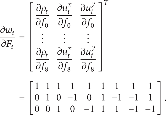
Since the flow field variables are functions of the distribution functions at time t, thus derivative ∂I _tx /∂F _t can be evaluated, using the chain rule, as follows:

${\frac{\partial I_{tx}}{\partial F_t}}^T={\frac{\partial I_{tx}}{\partial w_t}}^T\frac{\partial w_t}{\partial F_t},$

(56)

where derivative ∂I _tx /∂w _t can be evaluated using (38). To evaluate ∂w _t /∂F _t , using the conservation laws (8) and for ρ₀ = 1, we have

$\begin{array}{c}\frac{\partial w_t}{\partial F_t}={\left[\begin{array}{ccc}\frac{\partial {\rho }_t}{\partial f_{\mathrm{0}}}& \frac{\partial u_t^x}{\partial f_{\mathrm{0}}}& \frac{\partial u_t^y}{\partial f_{\mathrm{0}}}\\ ⋮& ⋮& ⋮\\ \frac{\partial {\rho }_t}{\partial f_{\mathrm{8}}}& \frac{\partial u_t^x}{\partial f_{\mathrm{8}}}& \frac{\partial u_t^y}{\partial f_{\mathrm{8}}}\end{array}\right]}^T\hfill \\ \hspace{1em}=\left[\begin{array}{ccccccccc}\mathrm{1}& \mathrm{1}& \mathrm{1}& \mathrm{1}& \mathrm{1}& \mathrm{1}& \mathrm{1}& \mathrm{1}& \mathrm{1}\\ \mathrm{0}& \mathrm{1}& \mathrm{0}& -\mathrm{1}& \mathrm{0}& \mathrm{1}& -\mathrm{1}& -\mathrm{1}& \mathrm{1}\\ \mathrm{0}& \mathrm{0}& \mathrm{1}& \mathrm{0}& -\mathrm{1}& \mathrm{1}& \mathrm{1}& -\mathrm{1}& -\mathrm{1}\end{array}\right].\end{array}$

(57)

For example, ∂I _tx /∂f₈ at time t is evaluated as

$\begin{array}{c}\frac{\partial I_{tx}}{\partial f_{\mathrm{8}}}=\frac{\partial I_{tx}}{\partial {\rho }_t}\frac{\partial {\rho }_t}{\partial f_{\mathrm{8}}}+\frac{\partial I_{tx}}{\partial u_t^x}\frac{\partial u_t^x}{\partial f_{\mathrm{8}}}+\frac{\partial I_{tx}}{\partial u_t^y}\frac{\partial u_t^y}{\partial f_{\mathrm{8}}}\hfill \\ \hspace{0.17em}=\left({\rho }_t-{\rho }_t^d\right)+\left(u_t^x-u_t^{x,d}\right)-\left(u_t^y-u_t^{y,d}\right).\end{array}$

(58)

Taking the derivative of both sides of (53) with respect to F _t , ∂Φ_{t + 1}/∂F _t is obtained:

$\begin{array}{c}\frac{\partial {\Phi }_{t+\mathrm{1}}}{\partial F_t}=\frac{\partial }{\partial F_t}\left[\left(\mathrm{1}-\beta \right)F_t+\beta F_t^{\text{eq}}+V\right]\\ =\left(\mathrm{1}-\beta \right)\frac{\partial F_t}{\partial F_t}+\beta \frac{\partial F_t^{\text{eq}}}{\partial F_t},\end{array}$

(59)

where

$\frac{\partial F_t}{\partial F_t}=\left[\begin{array}{ccc}\frac{\partial f_{\mathrm{0}}}{\partial f_{\mathrm{0}}}& \cdots & \frac{\partial f_{\mathrm{0}}}{\partial f_{\mathrm{8}}}\\ ⋮& \ddots & ⋮\\ \frac{\partial f_{\mathrm{8}}}{\partial f_{\mathrm{0}}}& \cdots & \frac{\partial f_{\mathrm{8}}}{\partial f_{\mathrm{8}}}\end{array}\right]=\left[\begin{array}{cccc}\mathrm{1}& \mathrm{0}& \cdots & \mathrm{0}\\ \mathrm{0}& \mathrm{1}& \cdots & \mathrm{0}\\ ⋮& ⋮& \ddots & \cdots \\ \mathrm{0}& \mathrm{0}& \cdots & \mathrm{1}\end{array}\right].$

(60)

Since the equilibrium distribution functions are functions of the flow field variables and also these variables are functions of the distribution functions, derivative ∂F _t ^eq/∂F _t can be evaluated, using the chain rule, as follows:

$\frac{\partial F_t^{\text{eq}}}{\partial F_t}=\frac{\partial F_t^{\text{eq}}}{\partial w_t}\frac{\partial w_t}{\partial F_t},$

(61)

where

$\begin{array}{c}\frac{\partial F_t^{\text{eq}}}{\partial w_t}=\left[\begin{array}{ccc}\frac{\partial f_{\mathrm{0}}^{\text{eq}}}{\partial {\rho }_t}& \frac{\partial f_{\mathrm{0}}^{\text{eq}}}{\partial u_t^x}& \frac{\partial f_{\mathrm{0}}^{\text{eq}}}{\partial u_t^y}\\ ⋮& ⋮& ⋮\\ \frac{\partial f_{\mathrm{8}}^{\text{eq}}}{\partial {\rho }_t}& \frac{\partial f_{\mathrm{8}}^{\text{eq}}}{\partial u_t^x}& \frac{\partial f_{\mathrm{8}}^{\text{eq}}}{\partial u_t^y}\end{array}\right]\hfill \\ \hspace{1em}=\left[\begin{array}{ccc}{w}_{\mathrm{0}}{\Theta }_{\mathrm{0}}& w_{\mathrm{0}}{\rho }_t\frac{\partial {\Theta }_{\mathrm{0}}}{\partial u_t^x}& w_{\mathrm{0}}{\rho }_t\frac{\partial {\Theta }_{\mathrm{0}}}{\partial u_t^y}\\ ⋮& ⋮& ⋮\\ w_{\mathrm{8}}{\Theta }_{\mathrm{8}}& w_{\mathrm{8}}{\rho }_t\frac{\partial {\Theta }_{\mathrm{8}}}{\partial u_t^x}& w_{\mathrm{8}}{\rho }_t\frac{\partial {\Theta }_{\mathrm{8}}}{\partial u_t^y}\end{array}\right]\end{array}$

(62)

and derivative ∂w _t /∂F _t was evaluated previously. For example, the derivative ∂f₈^eq/∂f₈ at time t is evaluated as follows:

$\begin{array}{c}\frac{\partial f_{\mathrm{8}}^{\text{eq}}}{\partial f_{\mathrm{8}}}=\frac{\partial f_{\mathrm{8}}^{\text{eq}}}{\partial {\rho }_t}\frac{\partial {\rho }_t}{\partial f_{\mathrm{8}}}+\frac{\partial f_{\mathrm{8}}^{\text{eq}}}{\partial u_t^x}\frac{\partial u_t^x}{\partial f_{\mathrm{8}}}+\frac{\partial f_{\mathrm{8}}^{\text{eq}}}{\partial u_t^y}\frac{\partial u_t^y}{\partial f_{\mathrm{8}}}\\ =w_{\mathrm{8}}\left[{\Theta }_{\mathrm{8}}+{\rho }_t\left(\frac{\partial {\Theta }_{\mathrm{8}}}{\partial u_t^x}-\frac{\partial {\Theta }_{\mathrm{8}}}{\partial u_t^y}\right)\right],\end{array}$

(63)

where

$\begin{array}{l}\frac{\partial {\Theta }_{\mathrm{8}}}{\partial u_t^x}=\mathrm{3}+\mathrm{9}\left(u_t^x-u_t^y\right)-\mathrm{3}{u}_t^x,\\ \frac{\partial {\Theta }_{\mathrm{8}}}{\partial u_t^y}=-\left[\mathrm{3}+\mathrm{9}\left(u_t^x-u_t^y\right)+\mathrm{3}{u}_t^y\right].\end{array}$

(64)

5.2.2. Evaluation of the Gradient Vector

Similarly, the gradient vector of the cost function with respect to the design variables vector as stated in Section 5.1.2 can be evaluated.

Remark 5. At the end of this section, it is clear that, compared to the discrete adjoint equation based on the NS equations, the present discrete adjoint equations (based on the LB equation) are extracted with less complexity, and therefore their implementation cost is lower. Moreover, the present derived adjoint equations have a simpler nature compared to the NS based adjoint.

6. Optimization Algorithm

After calculation of the gradient vector, we can change the values of the design variables using an optimization algorithm. The steepest descent algorithm was adapted to treat the design variables towards the optimum values. In the steepest descent algorithm, the design variables vector κ can be updated as

${\kappa }^{n+\mathrm{1}}-{\kappa }^n=-\alpha {\nabla }_{\kappa }I,$

(65)

where α is the step length. Using a linear search method, the step length is chosen such that the maximum reduction in the cost function is achieved [32]. Moreover, it can be found that the convergence of the gradient vector's norm to zero guarantees the convergence of the design variables to the optimum values, and consequently certain number of cycles required to reach the convergence of the optimization program is determined [1, 12, 32]. Algorithm 6 is a representation of the optimization procedure using the adjoint approach based on the LB method in the present work.

Algorithm 6 (optimization process using the adjoint approach based on the LB method). Consider the following.

Step 1 (define optimization problem).

• Select the cost function.

• Select the state variables vector (the governing equation).

• Select the design variables vector.

Step 2 (extract the main equations).

• Extract the MADA (or MIDA) equation.

• Extract the adjoint terminal condition.

• Extract the cost function gradient vector.

• Extract the partial derivatives of

Until reaching convergence of optimization algorithm:

Step 3 (solve the LB equation as forward in time).

• Set the initial conditions.

• Until reaching terminal time:

Step 4 (solve the MADA (MIDA) as backward in time).

• Set the adjoint terminal condition:

• Until reaching initial time:

Step 5 (evaluate gradient vector).

• Compute the partial derivatives of the cost function with respect to the design variables.

• Compute the partial derivatives of the governing equations with respect to the design variables.

Step 6 (modify design variables).

• Perform the steepest descent algorithm.

• Update the design variables vector.

7. Results and Discussion

In this section, the results of the MADA and MIDA equations for an elementary test case are presented. For complicated problems, the extraction and the evaluation procedure are similar.

7.1. Flow Field Inverse Optimization

The presented algorithm was implemented for the inverse optimization problem of an unsteady laminar poiseuille flow in an infinite channel with constant body forces. The simulation of the flow fieldwas performed using a 50 × 40 lattice. In this simulation, the periodic boundary conditions were applied on the inlet and outlet boundaries and the complete bounce-back scheme was used for applying the no-slip condition on the channel walls. Assuming a fluid with kinematic viscosity of 1 (giving λ = 3.5) and initial density of 1 throughout time t = 1,…, 100 in lattice unit where the fluid has an initial parabolic velocity profile with maximum value of u₀^{x, max⁡} = 0.1 along the horizontal axis and vertical velocity u₀ ^y = 0 in lattice unit, we consider the states of a flow driven by a constant body force κ ^d = [0.01, 0.002] as the desired or optimum states.

An interesting inquiry for the optimization problem to test the algorithm would be, on a fluid of a kinematic viscosity of 1, what driving force should one employ such as to influence the behavior of the states of the simulation for it to be as “close” as possible to those of the desired states? In other words, this problem tests whether the algorithm finds the solution that we already know which is obviously desired or optimum body force (design variable) κ ^d = [0.01, 0.002].

The stopping criterion for the convergence of the optimization algorithm is taken as ∥∇G∥ ≤ 10e − 7. Also, an arbitrary initial body force (design variable) κ = [0.04, 0] is chosen as a starting point for the iteration procedure of the steepest descent. All computations were performed on “Intel Core Due CPU T2450@ 2.00 GHz, 1 GB of RAM.”

Figure 3 shows the variation of the cost function versus number of optimization cycles for the inverse problem implemented by the MADA equation. This figure validates the convergence of the cost function. The main variations of the cost function approximately occur during the 5 initial cycles, and the cost function is reduced to 95.67 percent with respect to its initial value (the convergence of the cost function drops 2 orders of magnitude to a level of 4.564e − 02). After 20 cycles, the rate of convergence approaches zero (the convergence of the cost function drops 9 orders of magnitude to a level of 2.602e − 09). Finally, full convergence is obtained after 30 cycles.

Figure 3:

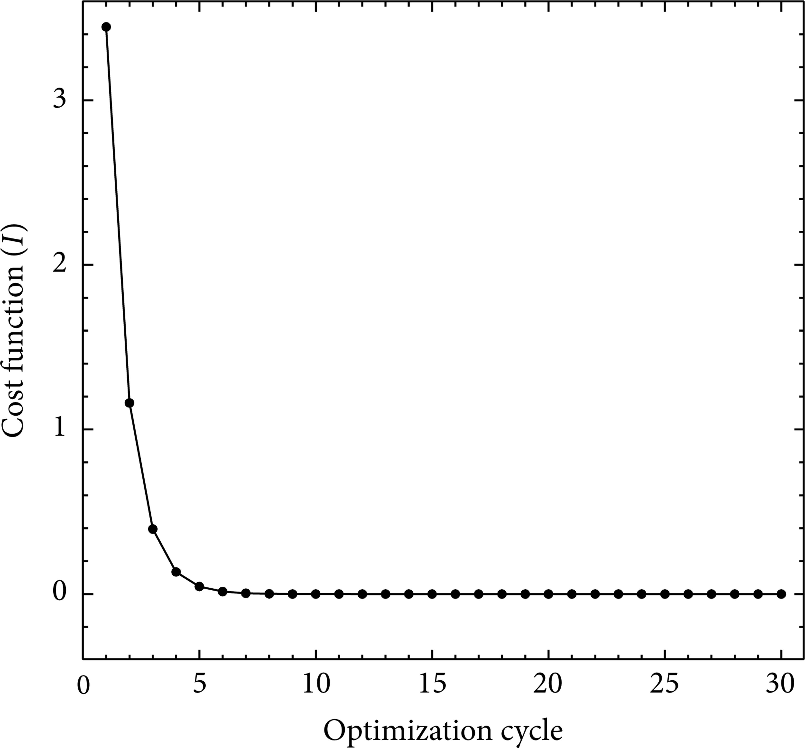
Convergence history of the cost function for the inverse optimization problem implemented by the MADA equation. Initial κ = [0.04, 0] and optimal κ ^d = [0.01, 0.002].

Figure 4 compares the variation of the cost function gradient with respect to the design variables versus number of optimization cycles for the inverse problem implemented by the MADA and MIDA equations. According to this figure, the convergence of the gradients is quite evident. The main variations of the gradients approximately occur during 10 initial cycles, and both gradients are reduced about 99 percent with respect to their initial values (the convergence of the gradient norm drops 2 orders of magnitude to a level of 5.371e − 02). After 30 cycles, the rate of convergence approaches zero (the convergence of the gradient norm drops 7 orders of magnitude to a level of 7.897e − 07). Also, this figure shows that the convergence rate of the optimization algorithm using both MADA and MIDA equations is the same and both of them evaluate the same gradients at each cycle.

Figure 4:

Comparison of convergence history of the gradient vector components for the inverse optimization problem implemented by the MADA and MIDA equations. Initial κ = [0.04, 0] and optimal κ ^d = [0.01, 0.002].

Figure 5 presents convergence history of the design variables to their optimal values during the optimization process using the MADA and MIDA equations. Both methods use the same flow solver to evaluate the flow variables and a similar procedure to calculate the adjoint variables. Therefore, it is expected that gradients assessed by the two methods in each optimization cycle will be identical. In fact, this adaption between the results obtained from the methods is showing the validation of the optimization algorithms implemented by the present approaches. It should be noted that convergence of the gradient vector norm is considered as the convergence criterion of the optimization program. According to the figures of the cost function and the gradients convergence history, it can be seen quite clearly that the cost function is converged faster than its gradient norm and approaches to the optimal value, while the design variables still have not been entirely converged to their optimal values. In other words, the convergence of the gradient vector norm of the cost function guarantees the full convergence of the cost function and the design variables. But, in general, the complete convergence of the cost function does not guarantee the complete convergence of design variables.

Figure 5:

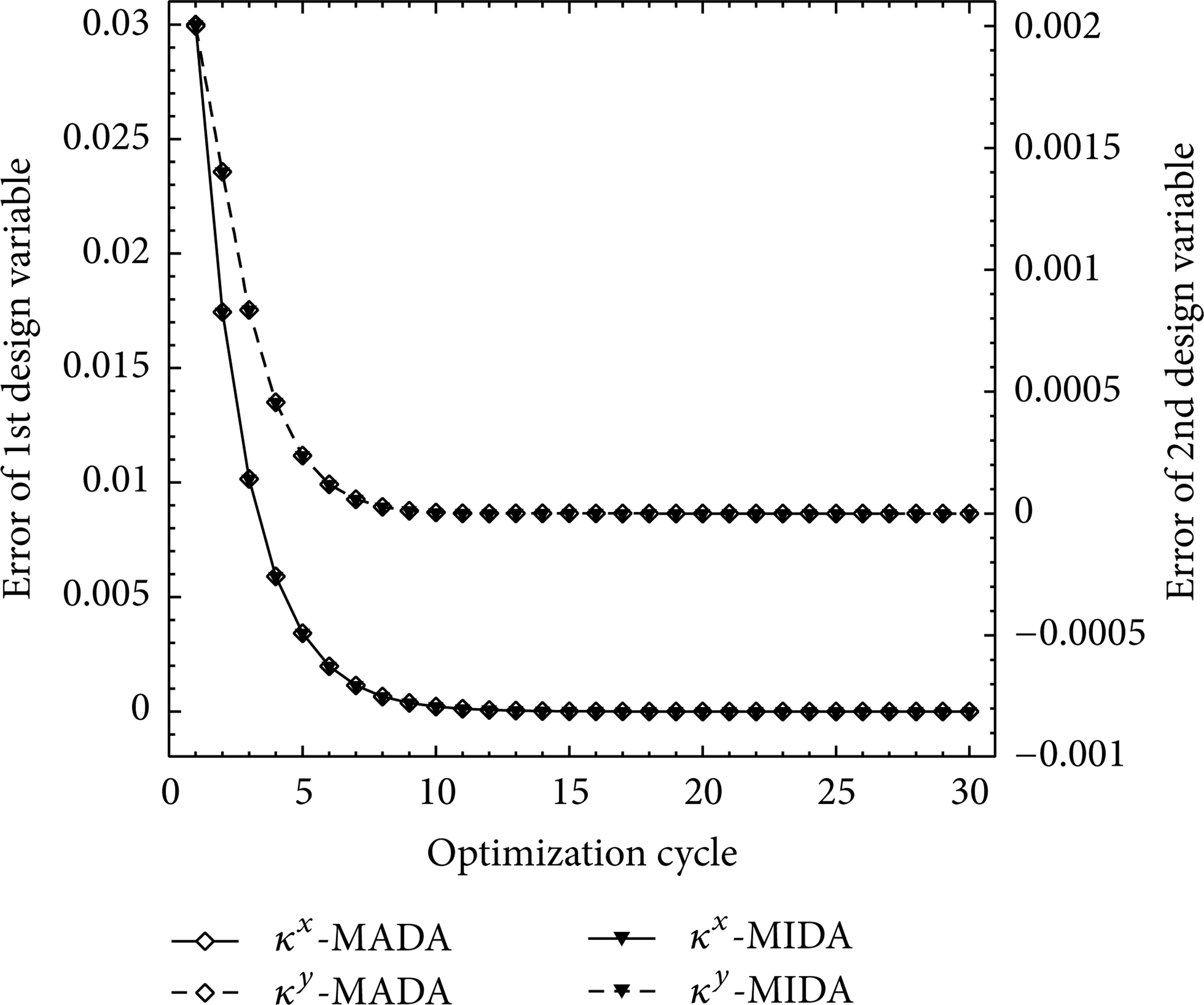
Convergence history of the design variables error (|κ − κ ^d |) for the inverse optimization problem implemented by the MADA and MIDA equations. Initial κ = [0.04, 0] and optimal κ ^d = [0.01, 0.002].

Remark 6. It should be noted that the convergence rate of the optimization program is strongly dependent on the step length of α in optimization algorithm. If a larger step size is selected, it would increase the convergence rate. But, adoption of a larger step length for α increases the variation of the design parameters and decreases the accuracy of the calculated gradients. Sometimes larger step length causes oscillatory behavior of the gradients. Moreover, adoption of smaller step length for α leads to an increase in number of optimization cycles [20, 33].

Figures 6 and 7 illustrate the gradients of the cost function with respect to the first and second design variables over subdomain [− 0.04, 0.04] × [− 0.004, 0.004], respectively. Based on these figures, the variation of the first design variable (the horizontal body force) has an almost linear effect on the flow field. Also, dependency of the flow field on the first design variable variations is far more than the second one. However, variations in the second design variable (the vertical body force) cause the nonlinear effects on the flow field in a way that these nonlinear effects have more increase at the large first design variables.

Figure 6:

Variations of the first component of the gradient vector in the inverse optimization problem implemented by the MADA equation. Optimal κ ^d = [0.01, 0.002].

Figure 7:

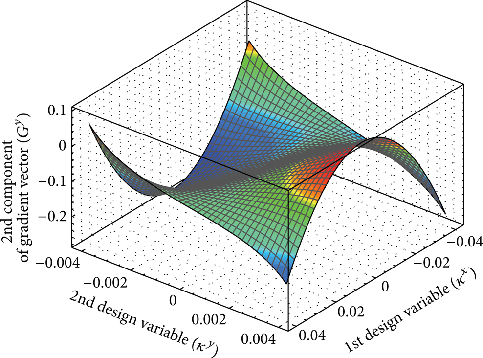
Variations of the second component of the gradient vector in the inverse optimization problem implemented by the MADA equation. Optimal κ ^d = [0.01, 0.002].

Figure 8 illustrates the contour map of the cost function over design variables subdomain [− 0.04, 0.04] × [− 0.004, 0.004]. It is clear in the map that the cost function attains its minimum at [0.01, 0.002]. The dashed line traces the path of the cycles obtained from the steepest descent algorithm. The points marked by + are the design variables generated by the algorithm at each cycle starting from the initial guess [0.04, 0] as it approaches [0.01, 0.002]. Therefore, we see that the steepest descent leads us to [0.01, 0.002], that is, to the point where the value of the cost function is minimal. It is important to note, however, that producing this map is extremely expensive since this requires the evaluation of the cost function for a good number of design variables to get an accurate shape of the cost function and it is not acceptable. This is being remedied by the steepest descent as it computes only the necessary evaluations to reach the optimal design variables.

Figure 8:

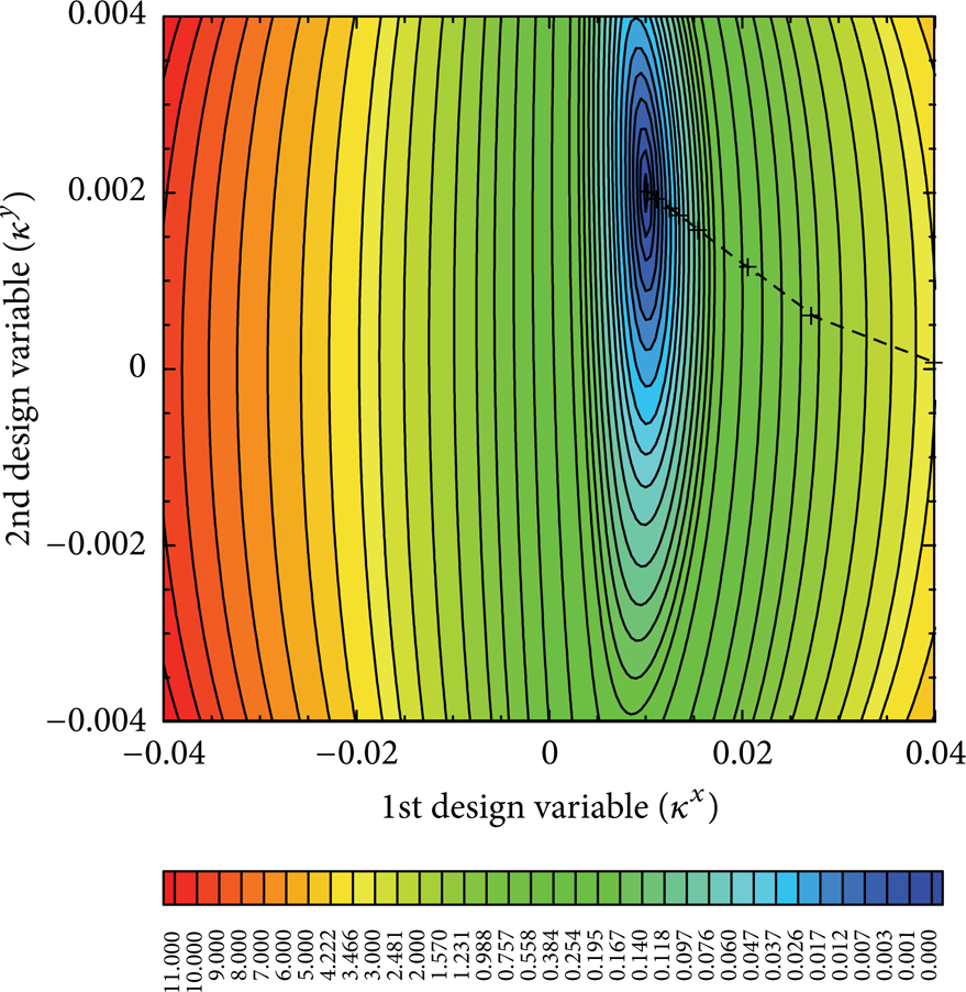
Contour map of the cost function for the inverse optimization problem implemented by the MADA equation. Optimal κ ^d = [0.01, 0.002].

7.2. Verification of the Optimization Results

It should be noted that the accuracy of the results obtained in the inverse problem, by itself, confirms the validity of the optimization program and it shows that the optimization algorithm has traveled in the correct path to such accurate results. However, for more certainty, the gradients obtained from the adjoint approach are compared with those of the central finite difference method (CFDM).

Remark 7. An estimate of the first derivative of a cost function I using CFDM is

${\nabla }_{\kappa }I\approx \frac{I\left(\kappa +\epsilon \right)-I\left(\kappa -\epsilon \right)}{\mathrm{2}\epsilon }+O\left({\epsilon }^{\mathrm{2}}\right),$

(66)

where ε is the step size. A small step size is desired to reduce the truncation error O(ε²) but a very small step size would also increase the subtractive cancellation errors. In order to produce an accurate finite difference gradient, a range of step sizes must be used, and thus the ultimate cost of producing n gradient evaluations with the CFDM is 2nr, where r is the number of different step sizes used to obtain a converged finite difference gradient (the used number of flow solvers is equal to 2nr). Therefore, the computational cost of the finite difference method for problems involving large numbers of design variables is both unaffordable and prone to subtractive cancellation error. But, in the adjoint method, according to (37), we can compute the gradient vector only with one flow solution in addition to one adjoint solution in each optimization cycle. The advantage is that (37) is independent from the flow field variables, with the result that the gradient of the cost function I with respect to an arbitrary number of design variables can be determined without the need for additional flow field evaluations.

To select an appropriate step size and compute the accurate gradients using the CFDM, several step sizes were examined. Table 1 shows the relative error of the gradients obtained from the MADA equation with respect to those of the CFDM for various step sizes at κ = [− 0.02, − 0.002].

Table 1:

Relative error of gradients obtained from the MADA equation (|(G^CFDM − G^MADA)/G^MADA|) in the inverse optimization problem at κ = [− 0.02, − 0.002]. Optimal κ ^d = [0.01, 0.002].

ε	G x -Relative error	G y -Relative error
10e − 04	3.63e − 02	1.73e − 01
10e − 05	1.09e − 03	3.37e − 02
10e − 06	4.33e − 05	6.29e − 05
10e − 07	2.71e − 07	8.78e − 07
10e − 08	8.94e − 08	1.00e − 09
10e − 09	8.35e − 09	2.29e − 10
10e − 10	8.02e − 09	9.42e − 10
10e − 11	6.22e − 08	9.61e − 09
10e − 12	9.35e − 07	1.20e − 07
10e − 13	7.42e − 06	6.58e − 06

The results illustrate the growth of subtractive cancellation error for ε ≤ 10e − 11 and the truncation error for ε ≥ 10e − 06. Also, good conformity can be seen between the results of these two methods for 10e − 10 ≤ ε ≤ 10e − 08. In Figure 9, we see that the proposed method is able to evaluate exactly the gradients of the cost function. Note that, in our discrete adjoint method implementation, for certain design variables, all the components of the gradient are computed within one forward sweep and one backward sweep as described in Section 5.1. In contrast, with the CFDM, we have to do one forward simulation with design variable κ + ε to obtain the macroscopic quantities and then solve for the value of cost function I(κ + ε), and finally perform another forward sweep for I(κ − ε).

Figure 9:

Comparison of the first component of gradient vector at κ ^y = 0.003 and the second component of gradient vector at κ ^x = 0.03 obtained from the MADA equation with those of the CFDM in the inverse optimization problem. Optimal κ ^d = [0.01, 0.002].

7.3. Comparison of the MADA and MIDA Equations Results

In Section 7.1, it was shown that the optimization process has exactly the same convergence rate using both MADA and MIDA equations. Also, the gradients evaluated by both equations match very well.

In Table 2, the number of optimization cycles and CPU time until convergence in the inverse optimization program implemented by the MADA and MIDA equations for the various grid sizes and the various numbers of designs variables are presented. For case I, the horizontal body force is used as the design variable with initial value κ ^x = 0.04 and optimal value κ ^x,d = 0.01, and for case II, the horizontal and vertical body forces are used as the design variables with initial value κ = [0.04, 0] and optimal value κ ^d = [0.01, 0.002]. It can be seen that the number of optimization cycles to reach convergence using both equations is the same. But the runtime of the optimization program until convergence using the MIDA equation, due to more calculations at each cycle, is little more than the MADA. Note that the number of optimization cycles in the program implemented by the MADA and MIDA equations is independent of the lattice size. This is due to the independency of the LB method from the chosen lattice. Moreover, the norm of gradient vector calculated in each optimization cycle is not affected by the number of lattice nodes. Here, the required number of cycles of optimization algorithm is only affected by the changes of initial design variables as a start point of optimization algorithm, desired design variables, cost function, and flow field. Increasing the number of the lattice nodes only increases the computational time in each optimization cycle. Besides, as it was expected, the total cost to obtain the gradients is independent of the number of design variables.

Table 2:

Number of cycles and CPU times (in sec) for the inverse optimization problem implemented by the MADA and MIDA equations for various grid size and number of design variables.

	Design variables	Lattice nodes	MADA		MIDA
			Cycle	CPU time	Cycle	CPU time
Case I	1	2000	30	5.623700e + 01	30	7.091500e + 01
	1	3000	30	1.584100e + 02	30	1.985600e + 02
	1	4200	30	5.052700e + 02	30	6.374300e + 02
	1	5600	30	1.958400e + 03	30	2.223800e + 03
Case II	2	2000	30	5.832900e + 01	30	7.291500e + 01
	2	3000	30	1.641100e + 02	30	2.045600e + 02
	2	4200	30	5.233100e + 02	30	6.554300e + 02
	2	5600	30	2.024500e + 03	30	2.277800e + 03

8. Conclusions and Future Work

In this research, the discrete adjoint approach using the LB method was implemented to solve the optimization problems of unsteady flow fields. First, the MADA and the MIDA equations and the cost function gradient vector were derived mathematically using the discrete LB equation. Also, for an elementary case, the analytical evaluation of the macroscopic and microscopic adjoint variables and the cost function gradients was presented. The investigation of the derivation procedure showed that the simplicity of the Boltzmann equation, as an alternative for the NS equations, facilitates the process of extracting the discrete adjoint equation. Therefore, the implementation cost of the adjoint equation based on the LB method is less than the adjoint equation based on the NS equations. This advantage can be effective in the optimization problems. Then, for the considered test case, the validity of the derived equations and the optimization procedure examined in an inverse optimization problem and the results obtained from the MADA and the MIDA equations were compared. The results show that the convergence rates of the optimization algorithm using both equations are identical and the evaluated gradients have very good agreement with each other. But the runtime of the optimization program to reach convergence using the MIDA equation is little more than the other one. Moreover, it has been shown that the number of optimization cycles in the program implemented by the MADA and the MIDA equations is independent of the lattice size and the number of design variables. Also, the total computational cost to obtain the gradients is independent of the number of design variables. According to the inherent characteristics of the LB method and the results obtained in this study, it can be received that combining the adjoint method and the LB method can serve as a useful and applicable tool in flow field optimization problems.

In this study, we have used a convenient and simplified form of the forcing term as the design variable in the optimization problem. Different representations of the forcing term have also been proposed (e.g., in [31] or [33]). Thus, more investigations may be needed to examine the effect of such forcing term on accuracy and stability of the LB method with regard to satisfying the incompressible NS equation. Also, for the optimization problem, the study was limited to a design variable that is constant throughout the space and time. Other cost functions may also be considered. Moreover, we have to note that changing the cost function will change the adjoint equation. In addition, the continuous adjoint equations can be derived using the continuous Boltzmann equation in space and time and the results can be compared to our findings. Besides, due to the local nature of the LB method, it is well suited for parallelization and GPU computing [34–36]. This capability of the LB method seems to be effective in efficiency of the adjoint methods and can be examined for (unsteady) optimization problems with a lot of constraints.

Conflict of Interests

The authors declare that there is no conflict of interests regarding the publication of this paper.