A Scheduled Activity Energy Aware Distributed Clustering Algorithm for Wireless Sensor Networks with Nonuniform Node Distribution

Abstract

Nonuniform node deployment makes the cluster-based routing protocol less efficient in wireless sensor networks (WSNs). Energy aware distributed clustering (EADC) is one of the cluster-based routing protocols proposed for networks with nonuniform node distribution, which can effectively balance the energy consumption among the nodes. However, due to the nonuniform node distribution, there is a redundancy in sensed and transmitted data in dense area. This unnecessary energy consumption is not considered in EADC. Therefore, in this paper, a new algorithm called scheduled activity EADC (SA-EADC) is proposed. SA-EADC exploits the redundant nodes and turns them off for the current round. The redundant nodes are scheduled based on their residual energy to work alternatively. The results show that SA-EADC significantly decreases the energy consumption and extends the network lifetime without degradation in coverage and sensing reliability of the network.

1. Introduction

Wireless sensor networks (WSNs) consist of a hundred to a thousand sensor nodes, which measure a property from the environment as well as processing and transmitting the collected data to the base station (BS) [1]. However, they have many constraints, because the sensor nodes have limited capabilities. Since the energy resources of the sensor nodes are limited and nonrechargeable, energy efficiency is a very critical issue in the design of the network topology, which affects the network lifetime significantly. Hence, the main concern in designing protocols is how to reduce the energy consumption and extend the network lifetime [2].

It has been proved by many researchers that among different categories of routing protocols based on the network architecture, cluster-based (hierarchical) routing protocols are more energy efficient and increase the scalability as well as lifetime of the network [3–5]. Clustering schemes divide the field into multiple clusters, where each cluster is controlled by a cluster head (CH) with the purpose of gathering data from cluster members (CM). CHs act as the local BS for their own clusters. After gathering data and performing data aggregation to omit the redundant data, the data are transmitted to the BS [6–8].

Networks with nonuniform node distribution make the cluster-based routing protocols less efficient [9, 10]. The nonuniform node deployment makes the energy consumption of the nodes more imbalanced [9]. Furthermore, as the density of the sensor nodes varies in each region due to nonuniform node distribution, in dense area the sensed and transmitted data are extremely correlated and redundant. In random and nonuniform node distribution, there may exist some redundant sensor nodes whose coverage areas are completely covered by their neighbor nodes. These redundant sensor nodes can be identified and scheduled to be activated alternatively in order to prolong the network lifetime [11].

Energy aware distributed clustering (EADC) [9] is one of the protocols proposed for networks with nonuniform node distribution, which can effectively balance the energy consumption among the nodes. However, the unnecessary energy consumption of redundant nodes is not considered in EADC. Therefore, in this paper, a scheduled activity energy aware distributed clustering (SA-EADC) is proposed based on EADC, which exploits the redundant nodes and turns them off. The redundant nodes are scheduled based on their residual energy to work alternatively. The proposed algorithm maintains the original sensing coverage and guarantees a certain redundancy. Consequently, SA-EADC avoids unnecessary redundant sensing and transmission of data, which reduces the overall energy consumption and extends the lifetime of the network.

The rest of the paper is organized as follows. Section 2 covers the related works in this area. Section 3 introduces the network model of our algorithm. Section 4 explains the used redundancy check method and activity-scheduling algorithm in SA-EADC. Section 5 presents SA-EADC in detail. Section 6 analyzes the properties of the proposed protocol. Section 7 describes the simulation and the analysis of the obtained results. Finally, the paper is concluded in Section 8.

2. Related Work

In this section, first some typical energy efficient clustering protocols are discussed. Afterwards, the sensor node scheduling algorithms are analyzed, which focuses on exploiting the redundant nodes and scheduling their activity.

2.1. Energy Efficient Clustering Protocols

Low energy adaptive clustering hierarchy (LEACH) [5] is a fundamental clustering algorithm, in which the sensor nodes independently elect themselves as the CH. The CHs are responsible to gather the data from their CMs, perform data aggregation to omit the redundant data, and transmit data to the BS using single hop communication. The nodes are selected as the CHs in turn with the purpose of evenly distributing energy expenditure in the network. Despite of being simple, the remaining energy of nodes is not considered as a parameter in CH selection. Moreover, it is not suitable for the large size networks. Thus, several cluster-based routing protocols were proposed so as to tackle the limitations of LEACH and improve its performance [13–15].

Energy efficient heterogeneous clustered (EEHC) routing protocol proposed by Kumar et al. [16] considers a network with the nodes, which differ in their energy level. CH selection and cluster formation are performed in a distributed method. The CH selection phase is performed based on the residual energy of the nodes. Nevertheless, the intercluster communication phase is performed in single hop and the residual energy of the nodes is not considered in CH selection.

Energy-aware data gathering (EADEEG) [17] is another clustering routing protocol, which is able to achieve a good CH distribution. The CHs are selected according to the residual energy of the nodes and the average residual energy of their neighbors in EADEEG. In spite of improving the network lifetime, EADEGG suffers from the existence of “isolated points” [4].

Yu et al. [4] proposed energy aware distributed unequal clustering (EADUC) routing protocol in order to solve the mentioned problem in EADEGG. EADUC assumes a network with heterogeneous nodes, which are different in energy resources. Additionally, the clusters are constructed in unequal sizes in EADUC, in order to solve the “hotspot” problem. The hot spot problem is related to the early death of CH nodes, which are closed to the BS. Therefore, the clusters near to the BS have smaller size to save more energy for intercluster communication.

Arranging cluster sizes and transmission ranges (ACT) proposed by Lai et al. [7] is a novel clustering routing protocol. ACT separates the network topology into multiple levels. The sizes of the clusters are the same in each level and are different from other levels. In other words, the clusters near to the BS are the smallest, whereas the largest clusters are the farthest ones from the BS to overcome the problem of “hot spot.” Since ACT avoids reclustering in each round, a cluster maintenance phase was proposed. Cluster maintenance phase consists of CH rotation based on energy threshold and cross-level data transmission. The results show that ACT can significantly increase the network lifetime. However, it does not address the coverage problem [7]. In addition, although cluster sizes are arranged according to energy consumption, the location of the newly selected CH strays from the ideal ones. This issue makes the distribution of energy fluctuate [18].

Coverage preservation clustering protocol (CPCP) [19] is a clustering protocol in which the clusters are constructed based on a group of coverage-aware metrics [2]. It considers a network with nonuniform node distribution. The main concern of CPCP is coverage preservation and it uses good CH selection technique. However, the network lifetime and balancing energy expenditure are not noted in detail in CPCP [9].

2.2. Sensor Activity Scheduling Protocols

In [20], Cardei and Du proposed a method in order to preserve full coverage of the area, in which the sensor nodes are divided into disjoint cover sets. These cover sets are active alternatively. Each cover set contains adequate number of active sensor nodes, which are essential to cover the monitoring area, meanwhile the rest of the sensor nodes are turned off. While, the rest of the sensor nodes are turned off. However, this scheme is based on a centralized approach. Therefore, it requires global synchronization overhead; besides it is not scalable in the networks with large size.

In PEAS [21], the sensor nodes use a simple rule in order to decide about their activity. The sensor node will be active if it cannot find another active node in its probing range. Otherwise, it will return to the sleep mode. PEAS does not require the nodes to maintain the neighbor state and location information. Therefore, it reduces the complexity. However, it does not guarantee a complete coverage preservation of the environment [22].

Tian and Georganas in [22] proposed a scheduling scheme, in which the sensor nodes decide about their state in a distributed manner, based on the obtained coverage information from their neighbors. In this scheme, in order to avoid creation of “blind points” in the network, a random back-off time is introduced, before a node makes a decision about its status. The problem of “blind points” occurs when two sensor nodes, whose redundancy is dependent to each other, decide to be inactive simultaneously.

In CPCP clustering scheme [19], in order to check the redundancy, the grid approach is used. Although this method is a straightforward approach and it does not limit the sensing coverage model, it can be time consuming, storage expensive, and computation complicated [12]. Soro and Heinzelman introduced a delay in node activation based on the nodes current cost value in order to avoid “blind point” problem. Therefore, the nodes with less cost have a better chance to be inactive.

In BCA clustering scheme [10], in order to identify inactive nodes, each CH calculates the average number of nodes in a cluster. The number of inactive sensor nodes is equal to the difference of the nodes in a cluster from the average number of nodes. The CHs select the inactive nodes randomly and each selected sensor node determines whether to be inactive or not. Although it is a simple method, the full coverage is not guaranteed in this approach.

3. Network Model

There are Nsensor nodes distributed in $M\times M$ square field in the network. Each node has a unique identity. The BS and the sensor nodes are stationary after deployment. Nodes are heterogeneous in terms of energy and location unawareness. All sensor nodes can use power control to vary the amount of transmit power. The BS is out of the field. It has sufficient energy resource and the location of the BS is known by each node. The communication link is symmetrical. The sensor nodes are able to estimate the distance between sender and receiver by the received signal strength indication. The sensor nodes are time synchronized and their failure is due to the energy depletion.

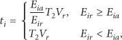
The energy model used in SA-EADC is adopted from LEACH [5]. In order to transmit l bit message to the distance of d, the energy dissipates as follows:

$$\begin{array}{cc}& E_{TX}\left(l,d\right)=\{\begin{array}{cc}l\times E_{\text{elec}}+l\times {\in }_{fs}\times d^{\mathrm{2}},\hfill & d\le d_{\mathrm{0}}\hfill \\ l\times E_{\text{elec}}+l\times {\in }_{mp}\times d^{\mathrm{4}},\hfill & d\ge d_{\mathrm{0}},\hfill \end{array}\end{array}$$

(1)

where $E_{\text{elec}}$ is the energy dissipation to run the radio electronics and ${\in }_{fs}$ and ${\in }_{mp}$ are the energy dissipation values to run the amplifier for close and far distances, respectively.

For receiving l bit message, the radio dissipates energy as follows:

$$\begin{array}{cc}& E_{RX}\left(l\right)=l\times E_{\text{elec}}.\end{array}$$

(2)

In addition, it is assumed that the energy consumptions due to data sensing and data aggregation are $E_{\text{sen}}$ and $E_{\text{com}}$ , respectively.

4. Sensor Activity Scheduling

In order to schedule the sensor activity to preserve the complete coverage of area, the first question is to find out whether the area covered by the sensor node is covered completely by its active neighbors. It should be noted that the state of the nodes' neighbor has a significant impact on the redundancy of the node. A node may not be redundant anymore, if one of its active neighbors becomes inactive. The second question is to identify the order of sensor's activation and deactivation [12]. The following sections describe the redundancy check method and activity scheduling procedure used in SA-EADC.

4.1. Redundancy Check Method

SA_EADC utilizes the crossing coverage redundancy check method proposed by Xing et al. [23] in order to determine the redundant nodes, since it reduces the storage requirements and computation complexity [12].

If the sensing disks of two nodes intersect each other, then crossing points that are the intersection points on the perimeters of two disks will be created. As represented in Figure 1, $S_2$ and $S_3$ disk perimeters created crossing point $P_1$ inside the sensing disk $S_1$ . The point on the sensing disk perimeter of a sensor is not considered as covered by the sensor itself. Thus, sensors $S_1$ and $S_2$ do not cover crossing point $P_1$ , whereas, $P_1$ is covered by $S_4$ . Consequently, $P_1$ is a covered crossing inside sensing disk of sensor $S_1$ . The redundancy rule of crossing coverage is explained as follows: “If all the crossings within the sensor's sensing disk are covered, then sensor S will be redundant and eligible to be inactive.” As it is shown in Figure 1, since all the crossing points inside sensing disk of $S_1$ are covered, it is a redundant node and it can go into sleep mode.

Figure 1

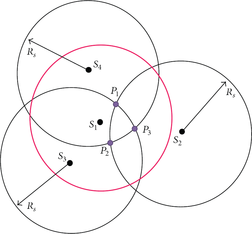
Crossing coverage redundancy check method [12].

4.2. Activity Scheduling Procedure

A fully distributed “self-inactivation” algorithm is proposed in order to determine the order of sensor's activation and deactivation and avoid creation of “blind points,” since the centralized algorithms are not scalable and need global synchronization overhead. The proposed algorithm avoids the problem of “blind points” by introducing the delay in the node deactivation based on the residual energy of the node. Therefore, the sensor nodes with higher remaining energy have a higher chance to be active in each round. The activity scheduling procedure of SA-EADC is discussed in detail in following section.

5. SA-EADC Algorithm

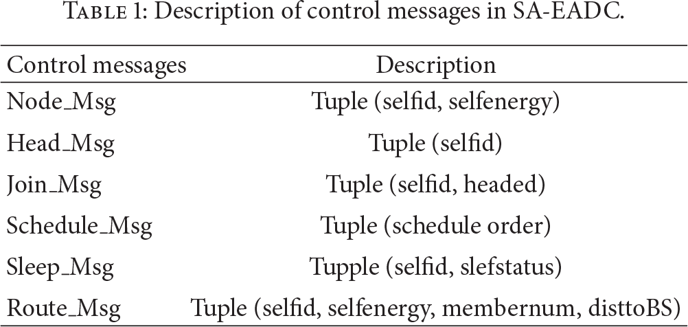
In this section, SA-EADC clustering algorithm is introduced in detail. Similar to EADC, the protocol contains an energy aware clustering algorithm (SA-EADC) and a cluster-based routing algorithm. SA-EADC adds a “sensor redundancy check and activation” phase to EADC. Thus, it makes even clusters. Furthermore, a subset of sensor nodes is selected to perform the sensing task while the redundant sensor nodes go to sleep mode for the current round. SA-EADC not only maintains the original coverage area, but also maintains a certain redundancy to guarantee the sensing reliability of the system. In the cluster-based routing algorithm, which is identical to [9], the energy consumption among the CHs is balanced. The description of the control messages used in the process of SA-EADC is shown in Table 1.

Table 1

Description of control messages in SA-EADC.

Control messages	Description
Node_Msg	Tuple (selfid, selfenergy)
Head_Msg	Tuple (selfid)
Join_Msg	Tuple (selfid, headed)
Schedule_Msg	Tuple (schedule order)
Sleep_Msg	Tupple (selfid, slefstatus)
Route_Msg	Tuple (selfid, selfenergy, membernum, disttoBS)

5.1. SA-EADC Details

The clustering process of SA-EADC is divided into four phases: information collection phase with duration of $T_1$ , cluster head competition phase with the duration of $T_2$ , sensor redundancy check and activation phase with duration of $T_3$ , and cluster formation phase with duration of $T_4$ .

5.1.1. Information Collection Phase

The duration of this phase is defined as $T_1$ , in which the status of all the nodes is set to “Active.” Identical to “information collection phase” in EADC, each node broadcasts a “Node_Msg.” This message consists of two values: the node ID and residual energy of the node within the radio range r. At the same time, each node receives “Node_Msg” messages from its neighbors. Afterwards, the sensor nodes start identifying their list of neighbors and build the list of active direct neighbors based on the received “Node_msg.” Two sensor nodes are called direct neighbor if $d(S_1,S_2)<2R_s$ , where $R_s$ is the sensing range of the sensor node.

Then each node starts to calculate the average residual energy of its neighbors $E_{ia}$ using

$$\begin{array}{cc}& E_{ia}=\frac{\mathrm{1}}{d}{\displaystyle \sum }_{j=\mathrm{1}}^d{E}_{jr},\end{array}$$

(3)

where $E_{jr}$ is the residual energy of $S_j$ (one neighbor node of $S_i$ ) and d is the number of the neighbors of $S_i$ . Afterwards, each node uses (4) in order to calculate its waiting time for broadcasting “Head_Msg”:

$$\begin{array}{cc}& t_i=\{\begin{array}{cc}\frac{E_{ia}}{E_{ir}}{T}_{\mathrm{2}}{V}_r,\hfill & E_{ir}\ge E_{ia}\hfill \\ T_{\mathrm{2}}{V}_r\hfill & E_{ir}<E_{ia},\hfill \end{array}\end{array}$$

(4)

where $t_i$ and $E_{ir}$ are waiting time and residual energy of $S_i$ , respectively, and $V_r$ is a real value uniformly distributed in $[\mathrm{0.9,1}]$ . This value is introduced to reduce the probability that two nodes simultaneously send the “Head_Msg.” The pseudocode of this phase is shown in Pseudocode 1.

Pseudocode 1: Pseudocode of information collection phase in SA-EADC.

begin (information collection algorithm)

    $state\leftarrow Candidate$

    $status\leftarrow Active$

   while ( $T_1$ has not expired) do

      Receive $Node\_Msg$

      Update neighborhood table NT $[$    $]$

      Update active direct neighbor table ADNT $[$    $]$

   end

    $t_i$ ← broadcast delay time for competing a cluster head

end

5.1.2. Cluster Head Competition Phase

Afterwards, SA-EADC starts the CH competition phase, whose duration is $T_2$ . In this phase, if the sensor node does not receive any “Head_Msg” during the expiration of timer $t_i$ , it will broadcast the “Head_Msg” in order to advertise itself as a CH within the radio range $R_C$ . Otherwise, the sensor node gives up the competition. Pseudocode 2 shows the pseudocode of this phase.

Pseudocode 2: Pseudocode of cluster head competition phase.

begin (cluster head competition algorithm)

   while ( $T_2$ has not expired) do

     if   $CurrentTime<t_i$   do

        if receive a $Head\_Msg$ from a neighbor NT $[j]$   do

             $state\leftarrow Plain$

            NT $[j]·state\leftarrow Head$

        else

            Continue

        end

     else if   $sate=Candidate$   do

         $state\leftarrow Head$

        Broadcast $Head\_Msg$

     end

   end

end

5.1.3. Sensor Redundancy Check and Activation Phase

As $T_2$ expires, SA-EADC begins the sensor redundancy check and activation phase whose duration is $T_3$ . During this phase, the plain nodes check their redundancy and their activity is scheduled. Note that the selected CH sensor nodes should be active in each round. Since all the sensor nodes know their state (i.e., plain or CH), all the non-CH nodes jointly participate in this phase without considering to which cluster they belong. This scheme prevents the redundant activation of sensors on the boundary of clusters, which may occur when the activation of nodes is performed independently in each cluster. Each plain node performs “crossing coverage” redundancy check method [23] to identify whether its complete coverage area is preserved or not. However, the edge nodes (i.e., the nodes that are placed at the boundary of the field) have no chance to be inactive, since all other nodes are located at one side of the edge nodes [22]. If the sensor node determines itself as the redundant, it will set a timer proportional to its residual energy level. Otherwise, its status will be remained as active for the current round. Note that when a redundant sensor node has higher residual energy level, its timer will last longer. Therefore, this sensor node has a higher priority to be active during the current round. Furthermore, setting the timer proportional to the energy level avoids creation of coverage holes. Furthermore, setting the timer proportional to the energy level avoids creation of coverage holes, because none of the redundant nodes will not go to sleep mode at the same time. Afterwards, the redundant nodes wait for timer expiration. If the sensor node receives no “Sleep_Msg” during its timer expiration, it will set its status to inactive, broadcast a “Sleep_Msg” in range of $2R_s$ , which includes the ID of the node and its status, and go to sleep mode for the current round. Otherwise, it will rebuild the list of its active direct neighbors and perform the redundancy check method again to determine whether it is redundant anymore or not. The pseudocode of this phase is shown in Pseudocode 3.

Pseudocode 3: Pseudocode of sensor redundancy check and activity scheduling phase.

begin (sensor redundancy check and activation algorithm)

 while ( $T_3$ has not expired) do

  if   $state=Plain$ and location ≠ on boundary do

   Execute the crossing coverage algorithm

    while ( $IsRedundant=True$ ) do

     Set Timer α   $E_{\text{residual}}$

     Wait for Timer expiration

      if receive a $Sleep\_Msg$ from an active direct neighbor do

       Update active direct neighbor table ADNT $[$    $]$

       Execute the crossing coverage algorithm

      else

       Broadcast $Sleep\_Msg$

        $Status\leftarrow Inactive$

      end

    end

  end

 end

end

5.1.4. Cluster Formation Phase

In this phase, all the active plain nodes select a CH, according to the received signal strength. Thus, they will select the nearest CH and send the “Join_Msg.” The CHs create a node-scheduling list based on the received “Join_Msg.” CHs create and send the “schedule_Msg” in order to identify the time of data transmission for the nodes and, in other times, they can be in the sleep mode. This issue will result in saving energy. Pseudocode 4 shows the pseudocode of cluster formation phase. At this point, the whole process of SA-EADC is done. The clusters consist of the nodes in Voronoi cell around the CHs.

Pseudocode 4: Pseudocode of cluster formation phase protocol analysis.

begin (cluster formation algorithm)

 while ( ${\mathrm{T}}_{\mathrm{4}}$ has not expired) do

  if   $state=Plain$ && $status=Active$ && has not sent $Join\_Msg$   do

   Send $Join\_Msg$ to the nearest cluster head

  else if   $state=Head$   do

   Receive $Join\_Msg$ from its $Active$ neighbor $Plain$ nodes

  end

 end

 if   $state=Head$   do

  Broadcast $Schedule\_Msg$

 end

end

5.2. Cluster-Based Routing Algorithm

SA-EADC utilizes the cluster-based routing algorithm of EADC [9]. Similar to EADC, the CHs generated by EADC distribute uniformly over the network. Therefore, the size of clusters is equal. However, due to the nonuniform node distribution, clusters in the dense area have more members in comparison to the clusters in the sparse area. Hence, this issue results in imbalanced energy consumption of CHs. According to Yu et al. [9] the energy consumption in multihop communication is divided into intracluster energy consumption and intercluster energy consumption. The CHs consume energy due to receiving, aggregating and transmitting data from their CMs, which is called intracluster energy consumption. In addition, they consume energy due to forwarding data for their neighbor CHs, which is called intercluster energy consumption. Yu et al. [9] adjusted the ratio of two parts of energy consumption, in order to balance the energy consumption among the CHs. The CHs in sparse area forward more data packet to mitigate the imbalance intracluster energy consumption. Furthermore, the heterogeneity of the nodes is also taken into consideration. Thus, if the CHs with higher residual energy are chosen to take more forwarding task, the network lifetime will be better prolonged.

At the beginning of this phase, each CH broadcasts a “Route_MSG” message within the radius range $R_r$ . This control message contains the values of remaining energy, the number of CMs, and the distance to the BS itself. If the distance of the CH to BS is less than an identified threshold, it will set the BS as its next hop. Otherwise, according to the received “Route_MSG,” it will choose a CH as the next hop with higher residual energy, smaller number of members, and no further away from BS. The value of “relay” is calculated using the following formula, when CH $S_i$ chooses CH $S_j$ as its next hop:

$$\begin{array}{cc}& \text{relay}\left(S_i,S_j\right)=\alpha \frac{E_{jr}}{E_{\max }}+\left(\mathrm{1}-\alpha \right)\frac{\mathrm{1}}{S_{j\left(\text{cm}-\text{num}\right)}},\end{array}$$

(5)

where $E_{jr}$ is the residual energy of the CH $S_j$ , $E_{\max }$ is the maximum initial energy of nodes in the network. $S_{j(\text{cm}-\text{num})}$ is the number of CMs of $S_j$ , and α is a real value uniformly distributed in $[\mathrm{0,1}]$ . It determines which factor is more important in selection of next hop. It is obvious from the equation that a CH with higher remaining energy and fewer CMs will have a larger value of “relay.” A neighbor CH with a highest “relay” and closer to the BS will be selected as the next hop. If there is more than one CH with equal and largest relay value, the one, which has a farther distance to the BS, will be chosen. The reason is to prevent premature death of the CHs near the BS because of forwarding much load. The pseudocode of this phase is shown in Pseudocode 5.

Pseudocode 5: Pseudocode of cluster-based routing algorithm.

begin (cluster-based routing algorithm)

 Broadcast $Route\_Msg$

 if   $disttoBS<DIST\_TH$   do

   $nexthop\leftarrow BS$

 else

  while ( $T_4$ has not expired) do

   Receive $Route\_Msg$

   Compute the value of $relay$

   Update cluster head neighborhood table CHNT $[$    $]$

  end

  if   $s_m$ has no cluster members do

    $nexthop\leftarrow s_m$

  else if   $s_j$ has max value of $relay$ in CHNT $[$    $]$   do

   Update MR $[$    $]$

  end

  if   $s_k$ has the max value of $disttoBS$ in MR $[$    $]$   do

    $nexthop\leftarrow s_k$

  end

 end

end

5.3. Data Transmission Phase

Data transmission phase is composed of intracluster communication and intercluster communication phase. These phases are discussed as follows.

5.3.1. Intracluster Communication Phase

CMs collect the data from the monitoring area and transmit the data in the allocated time slot to their CH directly.

5.3.2. Intercluster Communication Phase

CHs receive data from their members, perform data aggregation, and send the aggregated data to the next hop nodes. If a CH receives the data from other CHs, it will forward it to the next hop, without performing data aggregation. The topology of SA-EADC is shown in Figure 2.

Figure 2

Topology of SA-EADC.

6. Protocol Analysis

Theorem 1.

The overhead complexity of control messages in the network is $O(N)$ .

Proof.

In each clustering process, each node broadcasts a Node_Msg. Therefore, there are N Node_Msg. In each round, each active sensor node broadcasts a Join_Msg. Each CH broadcasts a Head_Msg, a Schedule_Msg, and a Route_Msg, while, each inactive node broadcasts a Sleep_Msg. Suppose the number of inactive sensor nodes and the number of generated CH are S and K, respectively. Therefore, the total number of control message in the whole network is $N+(N-K-S)+K+K+K+S=2N+2K$ , which is a linear function of N. Therefore, the overhead complexity of control messages in the network is $O(N)$ .

Theorem 2.

SA-EADC can set up the clustering topology in $O(1)$ time.

Proof.

SA-EADC is a distributed clustering algorithm. Therefore, the time complexity of the whole network is constant and is equal to a single node $O(1)$ . In other words, the time complexity is independent of the network size.

7. Performance Evaluation

A discrete event simulation (DES) in a purpose language C# was developed in order to perform the simulation. The simulations were conducted for two scenarios shown in Figure 3.

• (i)

Scenario 1: 100 nodes are deployed over an area of $200\times 200$  m² randomly. In this case, the locations of the sensor nodes are selected randomly.

(ii)

Scenario 2: 100 nodes are deployed over an area of $200\times 200$  m² nonuniformly. In this case, the sensor nodes are more grouped together in certain parts of the network.

Figure 3

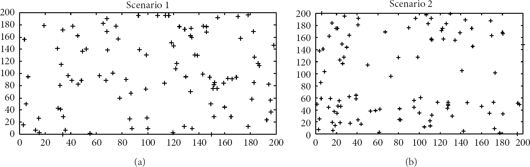
Network topology in two scenarios [9].

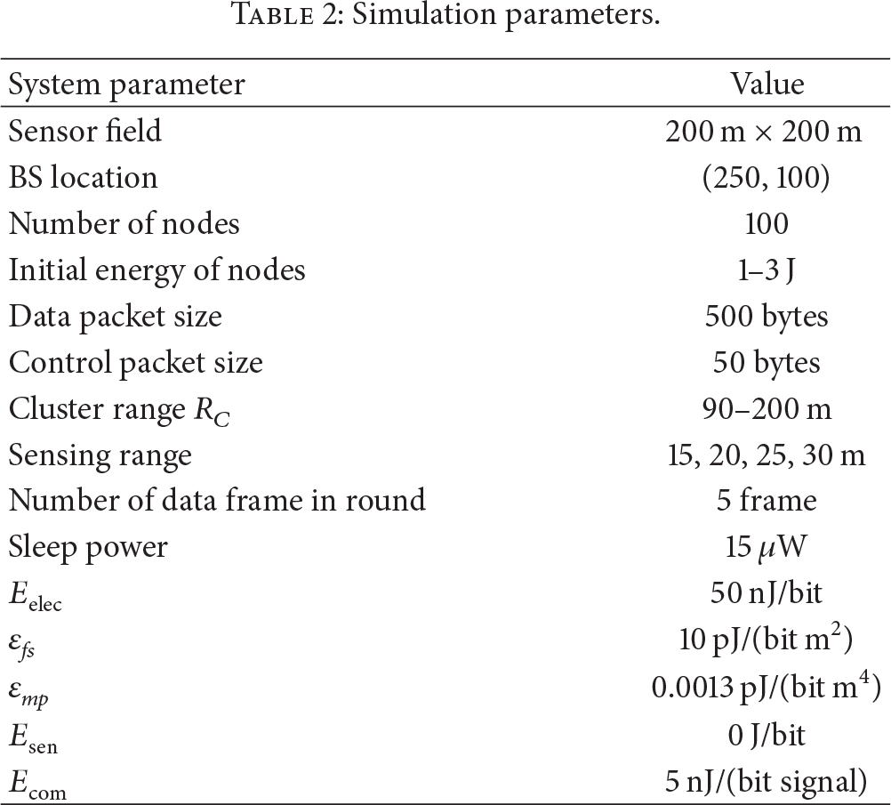
Every simulation result is the average of 100 independent experiments. The parameters of the simulation are listed in Table 2.

Table 2

Simulation parameters.

System parameter	Value
Sensor field	200 m × 200 m
BS location	(250, 100)
Number of nodes	100
Initial energy of nodes	1–3 J
Data packet size	500 bytes
Control packet size	50 bytes
Cluster range $R_C$	90–200 m
Sensing range	15, 20, 25, 30 m
Number of data frame in round	5 frame
Sleep power	15 μW
$E_{\text{elec}}$	50 nJ/bit
${\epsilon }_{\mathrm{fs}}$	10 pJ/(bit m2)
${\epsilon }_{\mathrm{mp}}$	0.0013 pJ/(bit m4)
$E_{\text{sen}}$	0 J/bit
$E_{\text{com}}$	5 nJ/(bit signal)

The performance of SA-EADC protocol is evaluated in two parts. The first is to evaluate the algorithm in terms of maintaining the sensing coverage and sensing reliability. The second is to study and analyze the effectiveness of the proposed clustering algorithm in terms of energy saving and network lifetime for the two stated scenarios. In addition, in order to investigate the effect of the sensing range on the different performance metrics, the sensing range was set between 15 and 30 m.

7.1. Coverage Preservation Evaluation

In this subsection, the performance of the SA-EADC based on its capability of preserving sensing coverage, remaining sensing reliability, and number of the inactive sensor nodes is evaluated in the two selected scenarios.

According to Tian and Georganas [22], in order to calculate the sensing coverage, the environment is divided into $1\hspace{0.17em}\text{m}\times 1\hspace{0.17em}\text{m}$ unit cells. It is assumed that the events occurred in the cells, where the events source placed at the center of the cells. Afterwards, the number of the nodes in EADC (i.e., original nodes) and the number of the active nodes in SA-EADC, which can detect the events, are calculated. If an event cannot be detected by any active node, but it is within the range of original sensing range, the event source is called a “blind point.” The existence of “blind points” means that the corresponding redundancy check and activation algorithm cannot preserve the original sensing coverage. Furthermore, the sensing degree of EADC and SA-EADC is computed. The sensing degree is defined as the number of nodes, which detect and report a single event at the same time. The sensing degree value represents the sensing reliability of the system.

7.1.1. Sensing Coverage

SA-EADC was run with sensing range $R_S$ of between 15 and 30 m in order to calculate the original sensing coverage and it obtained sensing coverage for both scenarios. As shown in Figure 4, with the increase of sensing range, the sensing coverage of the network is also increased. Moreover, in both scenarios, the obtained sensing coverage is equal to the original one. Hence, it shows that no blind point appears in the network as the eligible redundant sensor nodes become inactive by applying the sensor redundancy check and activation algorithm.

Figure 4

Network sensing coverage in scenario 1 and scenario 2.

7.1.2. Sensing Degree

In this section, the original sensing degree as well as the obtained sensing degree are calculated and compared in both scenarios. The space is still divided into $1\hspace{0.17em}\text{m}\times 1\hspace{0.17em}\text{m}$ with the event source located at the center of each cell. The ratio of number of the cells sensed by different active sensor nodes to the total number of the cell, when sensing range is 15, 20, 25, and 30 meter, was investigated.

Figure 5 shows the percentage of the deployed area that can be monitored with different sensing degrees in Scenario 1. As it is illustrated, the original sensing degree is varied from 1 to 9, from 1 to 11, from 1 to 12, and from 1 to 15 when the sensing range is 15, 20, 25, and 30, respectively. Whereas, the obtained sensing degree is always varied from 1 to 5, which shows that SA-EADC controls the redundancy and sensing degree of the network effectively. Similarly, Figure 6 illustrates that in Scenario 2 the sensing degree is varied from 1 to 9, from 1 to 11, from 1 to 16, and from 1 to 21 when the sensing range is 15, 20, 25, and 30, respectively, while, the obtained sensing degree is always varied from 1 to 6. Although SA-EADC turns off the redundant nodes, it still controls the redundancy and sensing degree of the network.

Figure 5

Different sensing degree of network in scenario 1.

Figure 6

Different sensing degree of network in scenario 2.

7.1.3. Inactive Sensor Nodes

In this section, the impact of sensing range and deployed node number over the number of inactive sensor nodes is investigated. In order to show the effect of varying sensing range on the number of inactive sensor nodes, in both scenarios, $R_S$ and $R_C$ were set between 15–30 m and 90–200 m, respectively. Figure 7 shows the average number of inactive sensor nodes per round in both scenarios. As shown in this figure, as long as the sensing range increases, there would be an upsurge in the number of inactive nodes. The increased sensing range (i.e., $R_S$ ) leads up to high probability of existence of the redundant sensor nodes, since their sensing coverage is also covered completely by the sensing coverage of their neighbors. Therefore, they will identify themselves as the redundant nodes and will be inactive for the current round if their sleep mode is not resulting in creating “blind points.”

Figure 7

Number of inactive nodes in each scenario.

Additionally, in order to investigate the effect of sensing range and node density on the number of inactive sensor nodes, the node density is changed by varying the sensing range from 15 to 30 m and the deployed node number from 100 to 250 in the same $100\times 100$ area. The variation of number of inactive sensor nodes along with variation of sensing range and node density is shown in Figure 8 in a 3D surface plot. Figure 8 shows that increasing the number of deployed nodes and increasing the sensing range will result in more numbers of inactive sensor nodes.

Figure 8

Number of inactive nodes versus node density.

7.2. Energy Consumption Evaluation

In this section, the ability of SA-EADC in terms of energy saving is evaluated for the two mentioned scenarios. Therefore, in order to perform this evaluation, the network lifetime and average energy consumption of the nodes per round are selected as the performance metrics.

7.2.1. Network Lifetime

The network lifetime is defined as the time (i.e., round) when 90 percent of the nodes are alive. In both scenarios, the cluster range (i.e., $R_C$ ) was set between 90 m and 200 m. Furthermore, in order to evaluate the effect of the sensing range on the network lifetime, the $R_S$ was set between 15 m and 30 m. Figures 9 and 10 show the relation between $R_C$ , $R_S$ , and network lifetime. As shown in these figures, SA-EADC increases the network lifetime as compared to EADC in the same simulation setting. Furthermore, with the increase of sensing range in SA-EADC, there is an increment in the network lifetime of the system.

Figure 9

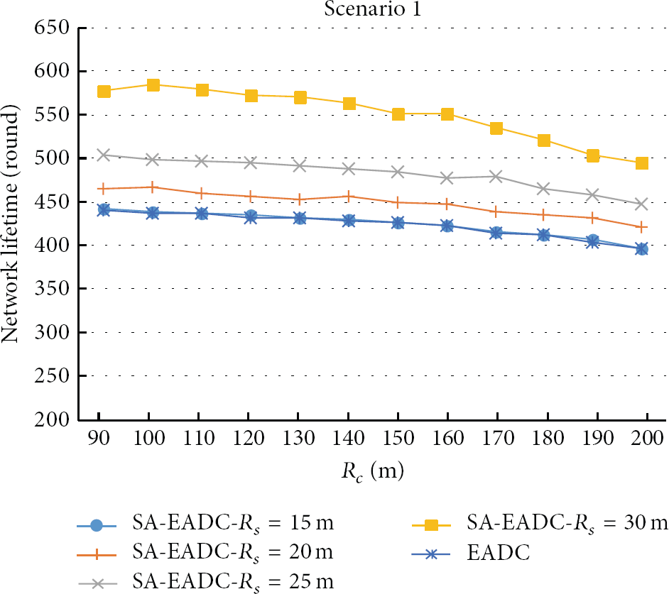
Network lifetime of scenario 1.

Figure 10

Network lifetime of scenario 2.

In Scenario 1, when the $R_S=15$  m, there is a slight (i.e., less than 1%) improvement in the network lifetime. While when the sensing range is 20 m and 25 m, the network lifetime improvement is 5% and 13%, respectively. Meanwhile, there is a significant raise in the network lifetime (i.e., 30 percent improvement) when $R_S$ is equal to 30 m.

Similarly, in Scenario 2, the network lifetime is increased slightly by 1.2% where $R_S=15$  m. In addition, the network lifetime improves by 4% and 7% when the sensing range is 20 m and 25 m, respectively. Furthermore, the network lifetime increased by 15% when the sensing range is equal to 30 m.

The reason of this appearance is that with the increase of $R_S$ , the number of redundant nodes, which are eligible to be inactive for the current round, increases. Therefore, more energy is saved when more nodes are inactive in each round. The results show that SA-EADC can effectively identify the redundant nodes and schedule them alternatively in a way that the network lifetime is prolonged.

7.2.2. Energy Consumption

The energy consumption is defined as the average energy that the nodes consumed during the topology construction, data transmission, and sleep mode per round. Similar to the previous sections, in both scenarios the cluster range (i.e., $R_C$ ) and sensing range (i.e., $R_S$ ) were set as 90–200 m and 15–30 m, respectively. Figures 11 and 12 show the relation among $R_C$ , average energy consumption, and the sensing range.

Figure 11

Average energy dissipation per round in scenario 1.

Figure 12

Average energy dissipation per round in scenario 2.

As it is presented in these figures, the average energy consumption of the sensors in each round gradually increases with the increase of the $R_C$ , due to the increment in the cluster size, and energy consumption of the CHs. It shows that the proposed clustering algorithm outperforms EADC in terms of average energy consumption in each round. The inactive nodes consume energy in the sleep mode. However, turning them off would result in reducing the energy consumption of the network. Furthermore, with the increase of the sensing range, the energy dissipation of the nodes decreases significantly.

As can be seen in Scenario 1, the energy consumption of the nodes improves slightly by 3.07%, when the sensing range is set to 15 m. While, the sensing range is set to 20 m and 25 m, the energy consumption recovers by 13% and 20%, respectively, compared to EADC. Eventually, there is a significant improvement (i.e., 27%) in energy consumption when $R_S=30$  m.

Similarly, in Scenario 2, the energy consumption is decreased slightly by 6% when $R_S=15$ . When the sensing range is 20 and 25, the energy dissipation of the nodes recovers by 14% and 18% in each round, respectively. Meanwhile, there is a momentous decline in the energy dissipation (i.e., 25% percentage improvement) when $R_S$ is equal to 30.

This phenomenon occurs due to the following reason: the number of redundant nodes, which are eligible to go to sleep mode, increases with the increase of sensing range. Therefore, with the decrease of active node in each round, the sensor nodes save more energy. The results show that SA-EADC can effectively identify the redundant nodes and schedule them alternatively in a way that the energy consumption of the network decreases.

8. Conclusion

In this paper, a clustering algorithm, namely, SA-EADC, based on EADC for wireless sensor network with nonuniform node distribution is proposed. The SA-EADC identifies the redundant nodes, whose sensing coverage area also is covered completely by their direct neighbors and turns them off. It schedules these sensor nodes based on their residual energy to be activated alternatively. The analysis and simulation results show that the proposed algorithm can effectively identify the redundant nodes and schedule them to be active in a way that reduces the overall energy consumption. Therefore, it extends the network lifetime as well as maintains the original sensing coverage of the network.