Output-Only Identification of System Parameters from Noisy Measurements by Multiwavelet Denoising

Abstract

In this paper we estimate the parameters of a multidimensional system from a record of noisy output measurements by using a multiwavelet denoising technique. In this output-only identification scheme, we extend wavelet denoising methods to the multiwavelet case. After the noise has been removed from the output records by wavelet methods, either full model identification or deterministic subspace identification can be performed. In the former case, full information on the system such as modal values and shapes becomes available by postprocessing. In the latter case, the observable modal values of the system as well as modal shapes at the sensor locations can be extracted from the identified parameters. Additionally, we discuss the requirements on the measuring devices to be compatible with wavelet transforms of a particular type. The validity and merit of the developed scheme are illustrated by examples of numerically simulated and experimentally measured signals, including comparisons with stochastic identification methods.

1. Introduction

The identification problem in structural and mechanical systems is addressed along two related tracks. The first track is represented by modal identification, which traverses a large number of applications. Modal identification is an essential technique for analysis, design, and diagnosis of structural systems. The technique aims at the identification of modal frequencies, mode shapes, and damping ratios. It serves to validate or numerically tune mathematical models and also to assess structural damage. The second track embraces parameter identification, which is primarily directed at structural health monitoring, damage detection, and structural modifications. In the latter case, the system mass, stiffness, and damping matrices are the target of the identification process.

In modal identification, two approaches are commonly employed. The first approach is a frequency domain modal identification, which is based on a measured frequency response function (FRF). This approach is sensitive to noise in the measured FRF, and therefore it is very difficult to find an FRF estimator that produces most accurate FRF data over the entire frequency range of interest [1]. Moreover, the current methods utilize graphical and curve-fitting methods, which often fail to distinguish between closely spaced modes or repeated modes. The second approach is a time domain modal identification, which is based on measured impulse response function (IRF). This approach utilizes the directly measured real-time acceleration and force signals, thus avoiding the transformation of measured raw data (time history) to data in the frequency domain for FRF. Unlike the FRF technique, the time domain approach uses response data either from known excitation sources or from ambient (unmeasurable) excitation. The latter feature is crucial in the identification of structures where a controlled excitation is not possible, for example, bridges, buildings, rotating equipment, and so forth. Time domain output-only modal identification methods utilize free vibration response estimates, including random decrement functions and response correlation functions obtained from response measurements [2]. Modal parameters are identified using time domain algorithms. These system identification algorithms include least-square methods [3], the Ibrahim time domain method [4], random decrement method [5], the Eigen system realization algorithm (ERA) [6], and stochastic subspace identification [7]. In addition to the aforementioned advantages, the time domain approach is capable of identifying closely spaced modes. On the other hand, the time domain approach suffers some weaknesses. It requires very high signal-to-noise ratio from the measured data [5]. The presence of measurements noise may result in some computational modes (fictitious modes) along with the identified structural modes.

On the other track, parameter identification provides direct information on the structural parameters, which is important to the development of reliability in structural controlled systems, as well as damage detection for structural health monitoring. Parameter identifications employ least-square methods, inverse solutions [8], and measured frequency response functions (FRF) [9]. In some investigations, the physical parameters have been identified using the result of the identified modal parameters [10].

In general, the measurements noise remained detrimental to the accuracy and fidelity of the identification process. Several techniques were invoked to improve the accuracy of the identification process by alleviating the problem of measurement noise. Some investigators utilized the powerful features of wavelets. Sone et al. [11] employed a wavelet transformation to perform identification of structural parameters based on acceleration measurements. Although they examined the influence of the observation noise on the accuracy of the estimated parameters, they did not invoke any denoising scheme. Instead, they suggested that accuracy could be improved by increasing the sampling density of the scale parameter. Nagarajaiah and Basu [12] presented an output-only modal identification using time frequency and wavelet techniques. They demonstrated the technique numerically on a structure excited by white noise; however, the investigation did not address the issue of noisy measurements.

Techniques for denoising measured signals were introduced in some medical and communications applications. These techniques included principal component analysis (PCA), independent component analysis (ICA), neural networks (NNs), adaptive filtering, empirical mode decomposition (EMD), and wavelet transforms. Although such techniques were utilized to enhance some direct measurements, for example, [13], they were not attempted within the context of system identification.

In an attempt to overcome some of the difficulties outlined above, we develop in this paper an output-only modal identification technique from output measurements of free vibration response by using truncated wavelet transforms and thresholding. The output measurements could be contaminated by noise from measurement errors and/or from ambient excitation. A wavelet transform breaks down the measured signal into components that correspond to “time” location and scale (frequency) level. Measurement errors are typically characterized by small coefficients of low scale (high frequency) components while ambient excitation appears as coefficients of low scale time localized components. The coefficients of the wavelet transform corresponding to scales up to a certain level are retained. This is done by truncating the wavelet series representation of the signal after a certain scale. The effect is to remove “most of” the ambient excitation and high frequency measurement errors. The low frequency measurement errors are then removed by wavelet thresholding. The wavelet thresholding method for multiwavelets in Section 3 is attempted for the first time.

The accuracy of the measuring device is ultimately related to the degree of smoothness of the wavelets to be used for the transformation. For example, the zero order hold (ZOH) devices provide a piecewise constant approximation of the measured signal. In this case, it suffices to use a db1 wavelet for the transformation of the signal. By contrast, averaging devices provide smoother approximation of the measured signal and smoother wavelets may be used, for example, db3 or db4. These issues are discussed in Section 2.

Section 4 discusses the state-of-the-art system identification techniques related to our problem. If output measurements are available for all system states, a full model identification is possible. This is the content of Section 4.1. In the more common situation, output measurements are available only at a few sensor locations optimally positioned on the system. In this case subspace techniques for parameter identification should be used. The use of multiwavelet denoising enables us to use deterministic subspace identification which is much faster and more accurate than stochastic subspace identification methods. The deterministic subspace identification method is discussed in Section 4.2 in the particular setting of our problem. Postprocessing of the identified parameters is presented in Section 4.3. For completeness and comparison purposes, we include an overview of the stochastic subspace identification method as well as the issue of the finite difference discretization of the continuous time derivatives in Sections 4.4 and 4.5.

In Section 5 we illustrate the various identification approaches considered in this paper with simulation examples and also experimental results.

2. From the Continuous to the Discrete Model

The free vibration deterministic equation of motion of a linear n-degree-of-freedom system is given by

$M\ddot{x}\left(t\right)+C\dot{x}\left(t\right)+Kx\left(t\right)=\mathrm{0},$

(1)

where $M,C,K\in {\mathbb{R}}^{n\times n}$ are the mass matrix, the damping matrix, and the stiffness matrix, respectively. $x(t)\in {\mathbb{R}}^n$ is the displacement. The first-order system equivalent of (1) is

$\dot{y}=Ay,$

(2)

where

$\begin{array}{c}y\left(t\right)=\left[\begin{array}{c}x\left(t\right)\\ \dot{x}\left(t\right)\end{array}\right]\in {\mathbb{R}}^{\mathrm{2}n},\\ A=\left[\begin{array}{cc}\mathrm{0}& I\\ -M^{-\mathrm{1}}K& -M^{-\mathrm{1}}C\end{array}\right]\in {\mathbb{R}}^{\mathrm{2}n\times \mathrm{2}n}.\end{array}$

(3)

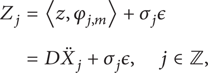
We consider here the general case of measurements taken by an array of r sensors of the n-dimensional acceleration $\ddot{x}(t)$ . Our goal is to identify the system matrix A from an r-dimensional output signal z(t) of measurements as follows:

$z\left(t\right)=D\ddot{x}\left(t\right),$

(4)

for some matrix $D\in {\mathbb{R}}^{n\times r}$ .

Measurements are usually taken at “discrete time” intervals. We then have a sequence of r × r matrices {Z _k }, where the (k, l) entry of each matrix Z _k represents the measurement made by sensor k of the measured component l at the time instant t _k , roughly speaking (see next subsection for more details). The common practice in signal treatment by wavelets is to regard the available sequence {Z _k } as coefficients of a signal approximating the original continuous time signal z(t) in a wavelet approximation space S _m . To clarify this point, assume that $\psi \in L_{\mathrm{2}}^r(\mathbb{R})$ is an r-dimensional wavelet vector and φ is its corresponding scaling-function vector. The approximation space S _m ⊂ $L_{\mathrm{2}}^r(\mathbb{R})$ is defined as the closure of the span of ${\{{\phi }_{k,m}\}}_{k\in \mathbb{Z}}$ , where

${\phi }_{k,m}\left(t\right)={\mathrm{2}}^{m/\mathrm{2}}\phi \left({\mathrm{2}}^{m}t-k\right).$

(5)

Then, the signal

$z_m\left(t\right)={\displaystyle \sum }_k‍Z_k{\phi }_{k,m}\left(t\right)$

(6)

is taken as an approximation to z(t). In the next subsection we discuss conditions for the validity of this practice.

2.1. Measurements as Wavelet Coefficients

Suppose we have r measuring devices that provide an r-dimensional output stream z(t). Let Ξ(t) be the r-dimensional vector of point spread functions of the measuring devices. Typical measurements are signal samples localized at time instants t _k ∈ [0, T]. The sampling process is commonly modeled as a convolution as follows:

$Z_k=〈z,{\mathrm{\Xi }}_{k,m}〉,$

(7)

where we assume that the time interval [0, T] is divided into 2 ^m equal subintervals and the values of the indexing integer k are properly restricted so that k/2 ^m ∈ [0, T]. Here, and elsewhere, we use the notation as follows:

$g_{k,m}\left(t\right)={\mathrm{2}}^{m/\mathrm{2}}g\left({\mathrm{2}}^{m}t-k\right),$

(8)

for any function $g:\mathbb{R}\to {\mathbb{R}}^p$ . Observe also that in (7) the inner product 〈·, ·〉 is matrix valued [14], for $f(t)\in {\mathbb{R}}^p$ and $g(t)\in {\mathbb{R}}^q$ , as follows:

$〈f,g〉:=\left[〈f_i,g_j〉\right]:={{\displaystyle \int }}_{\mathrm{0}}^T‍f\left(t\right)g{\left(t\right)}^{*}dt.$

(9)

Simple measuring devices implement a zero order hold (ZOH) in which case Ξ(t) = χ[0, T]_(t), the characteristic function for the interval [0, T]. Often discretization in this case is applied to system (2) to obtain the difference equation:

$Y_{k+\mathrm{1}}=Y_k+A{Y}_k\mathrm{\Delta },$

(10)

where Δ = T/2 ^m .

The point spread function, however, is not assumed, or expected, to be the scaling function of any wavelet. Therefore, the sampled signal (7) is not, strictly speaking, a sequence of wavelet approximation coefficients. The following discussion shows when this is possible.

We begin by considering the expansion of a signal $v\in L_{\mathrm{2}}^r(\mathbb{R})$ in a wavelet basis as follows:

$v={\displaystyle \sum }_{j,k\in \mathbb{Z}}‍c_{j,k}{\psi }_{j,k},$

(11)

where $\psi \in L_{\mathrm{2}}^r(\mathbb{R})$ is a mother wavelet [15] such that ${\{{\psi }_{j,k}\}}_{k,j\in \mathbb{Z}}$ is an orthonormal basis for $L_{\mathrm{2}}^r(\mathbb{R})$ and where ψ _j,k (t) = 2^k/2ψ(2 ^k x − j). The r × r wavelet coefficient matrix c _j,k is given by

$c_{j,k}=〈v,{\psi }_{j,k}〉.$

(12)

Parseval's identity gives

${\parallel v\parallel }_{L_{\mathrm{2}}^r\left(\mathbb{R}\right)}^{\mathrm{2}}={\displaystyle \sum }_{j,k\in \mathbb{Z}}‍{\parallel c_{j,k}\parallel }^{\mathrm{2}},$

(13)

where, for a matrix c = [c _l,m ²],

${\parallel c\parallel }^{\mathrm{2}}={\displaystyle \sum }_{l,m}‍c_{l,m}^{\mathrm{2}}.$

(14)

Alternatively, if $\phi \in L_{\mathrm{2}}^r(\mathbb{R})$ is the associated scaling function, we can expand v in terms of ${\{{\phi }_{j,m}\}}_{j\in \mathbb{Z}}$ and ${\{{\psi }_{j,k}\}}_{k>m,j\in \mathbb{Z}}$ , for some $m\in \mathbb{Z}$ , where φ _j,m (t) = 2^m/2φ(2 ^m x − j). The familiar approximation-detail representation of v is

$v={\displaystyle \sum }_{k>m,j\in \mathbb{Z}}{d}_{j,k}{\psi }_{j,k}+{\displaystyle \sum }_{j\in \mathbb{Z}}{c}_{j,m}{\phi }_{j,m},$

(15)

where d _j,k = 〈v, ψ _j,k 〉 and c _j,m = 〈v, φ _j,m 〉, and

${\parallel v\parallel }_{L_{\mathrm{2}}^n\left(\mathbb{R}\right)}^{\mathrm{2}}={\displaystyle \sum }_{k>m,j\in \mathbb{Z}}{\parallel d_{j,k}\parallel }^{\mathrm{2}}+{\displaystyle \sum }_{j\in \mathbb{Z}}{\parallel c_{j,m}\parallel }^{\mathrm{2}}.$

(16)

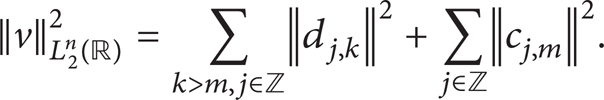
For the finite domain [0, T] we consider only nonnegative scales k ≥ 0 and translation values j such that the support of ψ _j,k is contained in [0, T]. Special attention has to be given as well to the end points in order to maintain the orthonormality of the basis vectors. Details of such considerations can be found in [15]. We will not include these details here in the interest in reducing the technicality of the presentation.

Now, to make the connection between the measured signal {Z _j } and the wavelet representation of the continuous time signal z, we assume that

$S_m=\mathrm{span}{\left\{{\phi }_{j,m}\right\}}_{j\in \mathbb{Z}}=\mathrm{span}{\left\{{\psi }_{j,k}\right\}}_{j\in \mathbb{Z},\mathrm{0}\le k<m}.$

(17)

The projection of z onto S _m is

$z_m={\displaystyle \sum }_{j\in \mathbb{Z}}‍〈z,{\phi }_{j,m}〉{\phi }_{j,m}$

(18)

$={\displaystyle \sum }_{\mathrm{0}\le k<m}‍\hspace{0.17em}{\displaystyle \sum }_{j\in \mathbb{Z}}‍〈z,{\psi }_{j,k}〉{\psi }_{j,k}.$

(19)

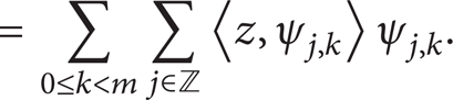
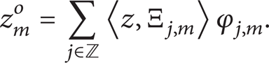
The first representation of z _m is known as the single scale representation while the second representation is known as the multiscale representation [15]. What we have available, however, are the measured values Z _j = 〈Ξ _j,m , z〉 rather than the coefficients 〈z, φ _j,m 〉. Therefore, our new “observed signal” is

$z_m^o={\displaystyle \sum }_{j\in \mathbb{Z}}‍〈z,{\mathrm{\Xi }}_{j,m}〉{\phi }_{j,m}.$

(20)

Accordingly, this introduces an error in the representation of z _m . Therefore, we may write

$\begin{array}{l}{z}_m=z_m^o+ϵ\\ \hspace{1em}={\displaystyle \sum }_{j\in \mathbb{Z}}‍〈z,{\mathrm{\Xi }}_{j,m}〉{\phi }_{j,m}+ϵ.\end{array}$

(21)

A principle was introduced in [16] that, whenever z _m is a polynomial of degree < ν, z _m ^o is also a polynomial of degree < ν. It was shown in [17] that this principle bounds the error ϵ in a reasonable way. The minimal assumptions on Ξ(t) for this to happen are the following.

1. Ξ(t) is bounded, ${\int }_{\mathbb{R}}‍\mathrm{\Xi }(t)dt=\mathrm{1}$ , and ${\int }_{\mathbb{R}}‍t^s\mathrm{\Xi }(t)dt\ne \mathrm{0}$ , s = 1, 2,…, ν.

2. The support of Ξ _j,m contains the point j/2 ^m and is contained in an interval of length ∼2^−m.

They simply mean that the point spread function has bounded support, is bounded, is translation invariant, and can distinguish between polynomials of degree < ν.

2.2. The Discrete Model

To relate to the actual system accelerations, we write

$\begin{array}{c}{z}_m={\displaystyle \sum }_{j\in \mathbb{Z}}‍Z_j{\phi }_{j,m}+ϵ\\ \hspace{1em}\hspace{1em}\hspace{0.17em}\hspace{0.17em}={\displaystyle \sum }_{j\in \mathbb{Z}}‍〈z,{\mathrm{\Xi }}_{j,m}〉{\phi }_{j,m}+ϵ\\ \hspace{1em}\hspace{1em}\hspace{0.17em}\hspace{0.17em}\hspace{0.17em}={\displaystyle \sum }_{j\in \mathbb{Z}}‍〈D{\ddot{x}}_m,{\mathrm{\Xi }}_{j,m}〉{\phi }_{j,m}+ϵ\\ \hspace{1em}\hspace{1em}\hspace{0.17em}\hspace{0.17em}\hspace{0.17em}={\displaystyle \sum }_{j\in \mathbb{Z}}‍D〈{\ddot{x}}_m,{\mathrm{\Xi }}_{j,m}〉{\phi }_{j,m}+ϵ\\ \hspace{1em}\hspace{0.17em}={\displaystyle \sum }_{j\in \mathbb{Z}}‍D{\ddot{X}}_k{\phi }_{j,m}+ϵ.\end{array}$

(22)

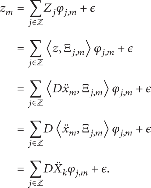
Other sources of errors, such as measurement errors, can also be added to the above equation. At the level of approximation m (i.e. in S _m ) we then get the following relation between the discrete coefficients:

$\begin{array}{c}{Z}_j=〈z,{\phi }_{j,m}〉+{\sigma }_jϵ\\ \hspace{1em}\hspace{0.17em}=D{\ddot{X}}_j+{\sigma }_jϵ,\hspace{1em}j\in \mathbb{Z},\end{array}$

(23)

where we may now assume that ϵ is N(0, γ) white noise and ${\sum }_{j\in \mathbb{Z}}‍{\sigma }_j=\mathrm{1}$ .

The sequence ${\{Z_j\}}_{j\in \mathbb{Z}}$ is further decomposed via the fast wavelet transform into detail coefficients corresponding to the representation of (19) producing noisy wavelet coefficients ${\{c_{j,k}\}}_{j\in \mathbb{Z},\mathrm{0}\le k<m}$ with ${\sum }_{j\in \mathbb{Z},\mathrm{0}\le k<m}‍{\parallel c_{j,k}\parallel }^{\mathrm{2}}<\infty$ as a result of Parseval's identity.

3. Noise Removal by Wavelet Thresholding

The goal of this section is to describe how to remove noise from a sequence $C={\{c_{j,k}\}}_{j\in \mathbb{Z},\mathrm{0}\le k<m}$ of noisy wavelet coefficient matrices of dimension r × r such as discussed in Section 2. This is done by finding a sequence $D={\{c_{j,k}\}}_{j\in \mathbb{Z},\mathrm{0}\le k<m}$ that minimizes the functional

${\parallel C-D\parallel }^{\mathrm{2}}+\lambda \parallel D\parallel ,$

(24)

for a predetermined value of the parameter λ. The term λ∥D∥, in the minimization problem above, has the effect of penalizing the norm of the solution sequence D and, therefore, tends to limit this norm by limiting the contributions of the small terms in the sequence. These terms usually correspond to low scale (high frequency) wavelet coefficients. For more details, see the work of Chambolle et al. [17] and DeVore and Lucier [18] on noise removal by wavelet thresholds. A treatment of the subject from a statistical point of view can also be found in [19]. Our work here addresses the multidimensional wavelet transforms (see [15] or [20] for definitions and properties).

The natural choice of the norm of a sequence $E={\{e_{j,k}\}}_{j\in \mathbb{Z},\mathrm{0}\le k<m}$ is

${\parallel E\parallel }^{\mathrm{2}}={\displaystyle \sum }_{j\in \mathbb{Z},\mathrm{0}\le k<m}‍{\parallel e_{jk}\parallel }^{\mathrm{2}}.$

(25)

Hence,

${\parallel C-D\parallel }^{\mathrm{2}}+\lambda \parallel D\parallel ={\displaystyle \sum }_{j\in \mathbb{Z},\mathrm{0}\le k<m}‍{\parallel c_{jk}-d_{jk}\parallel }^{\mathrm{2}}+\lambda {\displaystyle \sum }_{j\in \mathbb{Z},\mathrm{0}\le k<m}‍\parallel d_{jk}\parallel .$

(26)

The following discussion is an adaptation of the several approaches offered in [17] from which we choose the technique of wavelet soft thresholding because it combines effectiveness with relative simplicity.

To solve this minimization problem, we immediately notice that D should be chosen so that each of the terms ${\parallel c_{jk}-d_{jk}\parallel }^{\mathrm{2}}+\lambda \parallel d_{jk}\parallel$ is minimized separately. Thus, we end up with the generic problem of choosing d to minimize the functional

${\parallel c-d\parallel }^{\mathrm{2}}+\lambda \parallel d\parallel .$

(27)

Using elementary vector calculus, the necessary condition for the minimizer is

$\mathrm{2}d+\lambda \frac{d}{\parallel d\parallel }=\mathrm{2}c.$

(28)

To solve (28), we begin by taking norms on both sides to get

$\mathrm{2}\parallel d\parallel +\lambda =\mathrm{2}\parallel c\parallel .$

(29)

Hence,

$\parallel d\parallel =\parallel c\parallel -\frac{\lambda }{\mathrm{2}}.$

(30)

This means that we must choose d = 0 if ∥c∥ ≤ λ/2. If ∥c∥ > λ/2, we substitute ∥d∥ in (28) to get d = c(1 − λ/(2∥c∥)). Hence, the coefficients of the minimization problem at hand are given by

$d_{jk}=\{\begin{array}{cc}{c}_{jk}\left(1-\frac{\lambda }{\left(\mathrm{2}\parallel c_{jk}\parallel \right)}\right),\hfill & \parallel c_{jk}\parallel >\frac{\lambda }{\mathrm{2}},\hfill \\ \mathrm{0},\hfill & \parallel c_{jk}\parallel \le \frac{\lambda }{\mathrm{2}}.\hfill \end{array}$

(31)

Thus, denoising is achieved by setting to 0 all elements of C which are less than λ/2 in norm and shrinking towards zero all other coefficients.

This noise removal technique has two advantages.

1. All significant components are preserved. This is different from the usual series truncation after a specified number of terms. In this respect, this technique amounts to a nonlinear projection.

2. Possible noise in the significant components is removed by shrinking towards zero.

The estimation risk is defined as $E[{\parallel z_m-{\tilde{z}}_m\parallel }_{\mathrm{2}}^{\mathrm{2}}]$ , where z _m is given by (18) or (19) and ${\tilde{z}}_m$ is the signal constructed from the denoised sequence D. Then the penalty coefficient λ should be chosen to minimize the risk. It was shown in [17] that a near optimal value of the risk is achieved by the choice of the parameter λ as

$\lambda =\frac{a{\sigma }_{\mathrm{0}}}{{\mathrm{2}}^m},$

(32)

where σ₀² is the variance of the (zero mean) white noise and a is given by

$a=\sqrt{\ln {\mathrm{2}}^{\mathrm{2}m}-\mathrm{2}\ln \frac{{\parallel z\parallel }_{B_{\mathrm{1}}^{\mathrm{1}}\left(L_{\mathrm{1}}\left(I\right)\right)}}{{\sigma }_{\mathrm{0}}}}.$

(33)

Here, B₁¹(L₁(I)) is a Besov space in which the undiscretized signal z is assumed to exist.

4. Identification of the Denoised System

As discussed in the introduction, mechanical system identification is normally addressed in terms of modal characteristics, that is, to obtain its natural frequencies, mode shapes, and modal damping from measured frequency response functions due to known inputs either impulse or white noise. Alternatively, a time domain identification proceeds by estimating the system's mass M, damping C, and stiffness matrix K, at least up to a similarity transformation, from a record of measured accelerations and/or velocities and accelerations. In this case, modal characteristics can also be identified consequently. The wavelet transform approach combines the advantages of both worlds by being able to adjust to various frequency scales (through scale dilations) as well as zero in on time domain events (through time translations). As we have seen in Section 3, a carefully designed wavelet transform can be used to reduce noise in the measurements. After the noise removal process, identification can proceed more efficiently in the time domain using deterministic approaches, as will be discussed in the following subsections.

4.1. Full Model Identification

Theoretically, if we assume that all system accelerations can be measured, then we may proceed to compute the velocity and displacement via a numerical quadrature method. The order of the integrator is determined by the type of the wavelet used in the denoising process. For example, the wavelet db5 is estimated to be of class C² (i.e., continuous with two continuous derivatives). Because the denoised signal is a linear combination of these wavelets, it will also be of class C². In this case, a third-order (fourth for large time intervals) method is enough to use all the approximation accuracy that such a signal can provide.

With the denoised accelerations and the computed displacements and velocities at hand, the identification proceeds in a deterministic way starting from (2) where y is the noise-free output vector and A is the unknown coefficient matrix to be identified. Suppose we have a record of N ≥ 2n sampled data arranged in a 2n × N matrix form as

$\begin{array}{c}\left[y\right]=\left[\begin{array}{cccc}y\left(t_{\mathrm{1}}\right)& y\left(t_{\mathrm{2}}\right)& \cdots & y\left(t_N\right)\end{array}\right],\\ \left[\dot{y}\right]=\left[\begin{array}{cccc}\dot{y}\left(t_{\mathrm{1}}\right)& \dot{y}\left(t_{\mathrm{2}}\right)& \cdots & \dot{y}\left(t_N\right)\end{array}\right]\\ \hspace{1em}\hspace{1em}=\left[\begin{array}{cccc}Ay\left(t_{\mathrm{1}}\right)& Ay\left(t_{\mathrm{2}}\right)& \cdots & Ay\left(t_N\right)\end{array}\right]\\ \hspace{1em}\hspace{0.17em}=A\left[\begin{array}{cccc}y\left(t_{\mathrm{1}}\right)& y\left(t_{\mathrm{2}}\right)& \cdots & y\left(t_N\right)\end{array}\right]\\ \hspace{1em}\hspace{1em}=A\left[y\right].\hfill \end{array}$

(34)

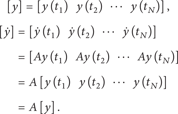
One can interpret this last equation as attempting to find A so that $[\dot{y}]$ is in the raw space of [y]. The best estimate [21] of A is then given by

$A=\left[\dot{y}\right]{\left[y\right]}^{†},$

(35)

where [y]_† is the Moore-Penrose right inverse of [y]. One may also take advantage of the special structure of the matrix A to eliminate the need to identify the already known matrices 0 and I. In this case we rewrite (1) in the form

$M^{-\mathrm{1}}C\dot{x}+M^{-\mathrm{1}}Kx=-\ddot{x}$

(36)

or in block matrix form as follows:

$\left[\begin{array}{cc}{M}^{-\mathrm{1}}K& M^{-\mathrm{1}}C\end{array}\right]\left[\begin{array}{c}x\\ \dot{x}\end{array}\right]=-\ddot{x}.$

(37)

Employing the Moore-Penrose inverse again, we get

$\left[\begin{array}{cc}{M}^{-\mathrm{1}}K& M^{-\mathrm{1}}C\end{array}\right]=-\left[\ddot{x}\right]{\left[y\right]}^{†},$

(38)

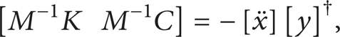
thus identifying M⁻¹K as the first n columns of the n × 2n matrix— $[\ddot{x}]{[y]}^{†}$ , and M⁻¹C as the next n columns.

4.2. Subspace Identification

To highlight the difference between our wavelet denoising identification technique and subspace identification methods, we shed the light on how the observations are treated in both cases. In large structures, it may not be possible to obtain measurements of all the outputs. Typically, sensors are installed at optimal locations in the structure where it is expected that all structural vibration modes are present in the measured data. These sensors can be accelerometers, velocity, or displacement transducers.

Subspace identification employs a state-space model, where the state equation is given by (1), or equivalently, (2), and the observation (or measurement) equation as follows:

$z\left(t\right)=C_a\ddot{x}\left(t\right)+C_v\dot{x}\left(t\right)+C_{d}x\left(t\right),$

(39)

where $z(t)\in {\mathbb{R}}^l$ are the outputs and C _a , C _v , $C_d\in {\mathbb{R}}^{l\times n}$ are the output matrices for the acceleration, velocity, and displacement, respectively. To simplify our discussion, we assume that the output sensors do not overlap. The more general case of overlapping sensors is discussed in [7]. See also [22] for a more recent overview of the subject. Substituting for the acceleration from the state equation, the output equation can be written as

$z\left(t\right)=Dy\left(t\right)+v\left(t\right),$

(40)

where $y=\left[\begin{array}{c}x\\ \dot{x}\end{array}\right],\mathrm{\hspace{0.17em}\hspace{0.17em}}D=\left[\begin{array}{cc}{C}_d-C_a{M}^{-\mathrm{1}}K& C_v-C_a{M}^{-\mathrm{1}}C\end{array}\right]$ , and v(t) is the measurement noise. Denoising the output measurements with multiwavelets enables us to write the observation equation in the following deterministic form:

$z\left(t\right)=Dy\left(t\right),$

(41)

and this way we deal with deterministic instead of stochastic identification. We should mention that subspace identification techniques recover the coefficient matrices up to a similarity transformation. We briefly overview the identification steps in what follows.

Since output signals are always measured at discrete time instants kΔt, we work with the sampled version of (2) and (41) as follows:

$\begin{array}{c}{y}_{k+\mathrm{1}}=A_d{y}_k,\\ z_k=D{y}_k,\end{array}$

(42)

where y _k = y(kΔt), z _k = z(kΔt), and A _d = exp⁡(AΔt). Finite difference discretization of (2) is also possible and will be discussed in the Section 4.4. Let

$Y_{\mathrm{0},N}=\left[\begin{array}{cccc}{y}_{\mathrm{0}}& y_{\mathrm{1}}& \cdots & y_N\end{array}\right]$

(43)

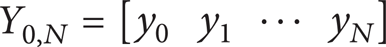
and define the block Hankel matrix as follows:

$Z_{\mathrm{0},s,N}=\left[\begin{array}{cccc}{z}_{\mathrm{0}}& z_{\mathrm{1}}& \cdots & z_{N-\mathrm{1}}\\ z_{\mathrm{1}}& z_{\mathrm{2}}& \cdots & z_N\\ \cdots & \cdots & \cdots & \cdots \\ z_{s-\mathrm{1}}& z_s& \cdots & z_{s+N-\mathrm{1}}\end{array}\right]\in {\mathbb{R}}^{ls\times N}.$

(44)

In general, we have n < s ≪ N. Also, define the extended observability matrix as follows:

$O_s=\left[\begin{array}{c}D\\ D{A}_d\\ ⋮\\ D{A}_d^{s-\mathrm{1}}\end{array}\right]\in {\mathbb{R}}^{ls\times n}.$

(45)

Then Z_{0, s,N} = O _s Y_{0, N}. Assuming that the pair (A, y₀) is reachable, the matrix Y_{0, N} has full rank. Therefore, the range spaces of Z_{0, s,N} and O _s are the same. Denote the SVD of Z_{0, s,N} by Z_{0, s,N} = U _n Σ _n V _n ^*, where ${\Sigma }_n\in {\mathbb{R}}^{n\times n}$ has full rank. Then, there is a change of base matrix T such that U _n = O _s T. It follows that

$D_T:=DT=U_n\left(\mathrm{1}:l,:\right)$

(46)

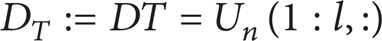
and the matrix A _T : = T⁻¹A _d T can be found by solving the overdetermined system U _n (1:(s − 1)l,:)A _T = U _n (l + 1:sl,:). Hence,

$A_T=U_n^{†}\left(\mathrm{1}:\left(s-\mathrm{1}\right)l,:\right)U_n\left(l+\mathrm{1}:sl,:\right).$

(47)

4.3. Postprocessing

We assume now that the coefficient matrix A of (35) or the state matrix A _T of (47) has been identified. The dynamic behavior of system (2) is completely characterized by the eigenvalues of A. In the case of the full model identification, these eigenvalues can be readily obtained. In the state-space model, the eigenvalues of A are related to those of A _T by

${\lambda }_k=\frac{\ln {\lambda }_k^T}{\mathrm{\Delta }t},\hspace{1em}\mathrm{1}\le k\le n.$

(48)

The eigenvectors of A are related to those of A _T by v _k = Tv _k ^T , 1 ≤ k ≤ n. The mode shapes at the sensor locations are the observed parts of the system eigenvectors and are related to the eigenvectors of A _T by

${\phi }_k=D_T{v}_k^T,\hspace{1em}\mathrm{1}\le k\le n.$

(49)

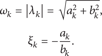
Furthermore, the mode frequency ω _k and damping ratio ξ _k can be extracted from the complex eigenvalue λ _k = a _k + ib _k of A by

$\begin{array}{c}{\omega }_k=\left|{\lambda }_k\right|=\sqrt{a_k^{\mathrm{2}}+b_k^{\mathrm{2}}},\\ {\xi }_k=-\frac{a_k}{b_k}.\end{array}$

(50)

4.4. Stochastic Subspace Identification

Since we intend to compare the results obtained by wavelet thresholding to those obtained with stochastic subspace methods, we briefly describe the stochastic approach using Kalman filters. A detailed discussion of the method can be found in [7, 23]. We assume stationarity and ergodicity. Let Λ _s = E[z_{k + s}z _k ^*] and G = E[z _k , y _k ^*]. Arrange the covariances Λ _s in a block Toeplitz matrix as follows:

$\mathcal{T}=\left[\begin{array}{cccc}{\mathrm{\Lambda }}_s& {\mathrm{\Lambda }}_{s-\mathrm{1}}& \cdots & {\mathrm{\Lambda }}_{\mathrm{1}}\\ {\mathrm{\Lambda }}_{s+\mathrm{1}}& {\mathrm{\Lambda }}_s& \cdots & {\mathrm{\Lambda }}_{\mathrm{2}}\\ \cdots & \cdots & \cdots & \cdots \\ {\mathrm{\Lambda }}_{\mathrm{2}s-\mathrm{1}}& {\mathrm{\Lambda }}_{\mathrm{2}s-\mathrm{2}}& \cdots & {\mathrm{\Lambda }}_s\end{array}\right].$

(51)

It can be shown that

$\mathcal{T}=\left[\begin{array}{c}D\\ D{A}_d\\ ⋮\\ D{A}_d^{s-\mathrm{1}}\end{array}\right]\left[\begin{array}{cccc}{A}_d^{s-\mathrm{1}}G& A_d^{s-\mathrm{2}}G& \cdots & G\end{array}\right]=O_s{C}_s.$

(52)

The SVD decomposition $\mathcal{T}=U_n{S}_n{V}_n$ is then used to obtain D and A _d , up to a similarity transformation T, via (46) and (47).

The Kalman filter estimates ŷ _k of the state vectors y _k can then be obtained using the familiar Kalman filter equations (see [14, 21, 23]).

4.5. Finite Difference Approximation

In this subsection we comment on the use of finite difference methods for the approximation of (2). These comments are motivated by our numerical experiments on using finite difference methods to discretize the state equation (2) of Section 5.3 below. In general, we have one of the two approaches: explicit schemes or implicit schemes. In an explicit scheme, we replace (2) with the discretized version as follows:

$\frac{X_{k+\mathrm{1}}-X_k}{\mathrm{\Delta }t}=A{X}_k,$

(53)

where X _k is the finite difference approximation of y(t _k ) and Δt is the time step. This equation leads to the discrete state equation as follows:

$X_{k+\mathrm{1}}=\widehat{A}{X}_k,$

(54)

where

$\widehat{A}=\left(I+\mathrm{\Delta }tA\right).$

(55)

We observe that (I + ΔtA) is a first-order approximation for exp⁡(ΔtA). This scheme is conditionally stable and, for small values of Δt, the eigenvalues of  become close to the border of the unit disc because I + ΔtA∼I. As a result, numerical errors start to blur the results of the identification algorithm. In an implicit finite difference method, (2) is replaced by

$\frac{X_{k+\mathrm{1}}-X_k}{\mathrm{\Delta }t}=A\left(\theta X_{k+\mathrm{1}}+\left(\mathrm{1}-\theta \right)X_k\right),$

(56)

where θ ∈ (0, 1]. This equation leads to the discrete model in (54) with

$\widehat{A}={\left(I-\theta \mathrm{\Delta }tA\right)}^{-\mathrm{1}}\left(I+\left(\mathrm{1}-\theta \right)\mathrm{\Delta }tA\right).$

(57)

This scheme is unconditionally stable and relatively large values of Δt can be taken to keep the eigenvalues of  away from the border of the unit disc. However, large values of Δt result in longer time taken to obtain good estimates of the system parameters. This may not be desirable for online identification systems.

The eigenvalues ${\widehat{\lambda }}_k$ of  are related to the eigenvalues λ _k of A by

${\widehat{\lambda }}_k=\frac{\mathrm{1}+\left(\mathrm{1}-\theta \right)\mathrm{\Delta }t{\lambda }_k}{\mathrm{1}-\theta \mathrm{\Delta }t{\lambda }_k},\hspace{1em}\mathrm{1}\le k\le n,$

(58)

which shows that the continuous time system is stable if and only if the discrete time system is stable.

5. Numerical Simulation

We consider the generic lumped-parameter mass-spring-damped system, with $M=\mathrm{diag}\left[\begin{array}{ccc}{m}_{\mathrm{1}}& m_{\mathrm{2}}& m_{\mathrm{3}}\end{array}\right]$ , as follows:

$\begin{array}{c}K=\left[\begin{array}{ccc}{k}_{\mathrm{1}}+k_{\mathrm{2}}& -k_{\mathrm{2}}& \mathrm{0}\\ -k_{\mathrm{2}}& k_{\mathrm{2}}+k_{\mathrm{3}}& -k_{\mathrm{3}}\\ \mathrm{0}& -k_{\mathrm{3}}& k_{\mathrm{3}}+k_{\mathrm{4}}\end{array}\right],\\ C=\left[\begin{array}{ccc}{c}_{\mathrm{1}}+c_{\mathrm{2}}& -c_{\mathrm{2}}& \mathrm{0}\\ -c_{\mathrm{2}}& c_{\mathrm{2}}+c_{\mathrm{3}}& -c_{\mathrm{3}}\\ \mathrm{0}& -c_{\mathrm{3}}& c_{\mathrm{3}}+c_{\mathrm{4}}\end{array}\right].\end{array}$

(59)

To simulate data measurements we used the parameter values as follows:

$\begin{array}{c}M=\mathrm{diag}\left[\begin{array}{ccc}\mathrm{1}& \mathrm{1}& \mathrm{1}\end{array}\right],\\ \left[\begin{array}{cccc}{k}_{\mathrm{1}}& k_{\mathrm{2}}& k_{\mathrm{3}}& k_{\mathrm{4}}\end{array}\right]=\left[\begin{array}{cccc}\mathrm{10}& \mathrm{50}& \mathrm{50}& \mathrm{50}\end{array}\right],\\ \left[\begin{array}{cccc}{c}_{\mathrm{1}}& c_{\mathrm{2}}& c_{\mathrm{3}}& c_{\mathrm{4}}\end{array}\right]=\left[\begin{array}{cccc}\mathrm{50}& \mathrm{50}& \mathrm{50}& \mathrm{10}\end{array}\right].\end{array}$

(60)

And the system is excited by the initial condition ${\left[\begin{array}{cccccc}\mathrm{1}& \mathrm{0}& \mathrm{0}& \mathrm{0}& \mathrm{0}& \mathrm{0}\end{array}\right]}^{*}$ .

5.1. Full Model Simulation

Simulated acceleration measurements of 1024 samples were generated in the interval [0, 1]. In order to allow for numerical integration to generate velocities and displacements, 16 internal nodes were generated between each pair of data samples. The numerical integration was implemented on the sampled data using a Newton-Cotes closed formula of order n = 4 (see, e.g., [24]), which would require 16 internal nodes to carry out numerical integration twice. The sampled accelerations were contaminated with N(0, 16) white noise, which resulted in a signal-to-noise (max(signal)/max(noise)) ratio of about 10. The contaminated signal was denoised using the MATLAB wavelet denoising function “wden” with a minimax selection rule for the threshold parameter and a db4 wavelet vector. The denoised signal was then numerically integrated twice to obtain velocities and displacements. An estimation $\tilde{A}$ of the system parameter matrix A was next computed using (35). The relative error in the estimation was then calculated using the following formula:

$\frac{{\max }_{i,j}\left(\left|A_{ij}-{\tilde{A}}_{ij}\right|\right)}{{\max }_{i,j}\left(\left|A_{ij}\right|\right)}.$

(61)

200 Monte-Carlo simulations resulted in a relative error of 1%. Figure 1 shows the results for the first component of the acceleration vector $\ddot{x}$ . Figure 1(a) shows the true acceleration signal. Figure 1(b) shows the simulated measured signal with noise. Figure 1(c) shows the signal after noise reduction by wavelets. Figure 1(d) shows the displacement signal obtained by numerically integrating the acceleration signal twice.

Figure 1:

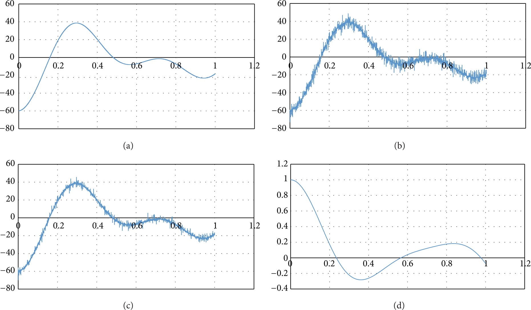
Some numerical results for the first component. (a) The original acceleration signal. (b) The simulated measured signal with noise. (c) The result of noise reduction by wavelets. (d) The displacement obtained by two numerical integrations.

We should note here that, in the noise reduced signal, only noise components above the threshold values are removed. We should also note the smoothing effect that numerical integration has on the signal. This is due to the fact that the integrals needed to recover the velocity and displacement signals are equivalent to denoising with Haar and linear spline scaling functions, respectively. High frequency noise components are orthogonal to such functions, which means that their integrals against either of these functions are 0.

5.2. Subspace Identification

200 Monte-Carlo simulations for the 6-dimensional structure above were performed using the deterministic subspace identification algorithm outlined in Section 4.2 with a state-output matrix as follows:

$D=\left[\begin{array}{cccccc}\mathrm{1}& 0.\mathrm{2}& 0.\mathrm{3}& \mathrm{0}& \mathrm{0}& \mathrm{0}\\ \mathrm{0}& 0.\mathrm{1}& \mathrm{0}& \mathrm{0}& \mathrm{0}& \mathrm{1}\\ \mathrm{0}& \mathrm{0}& \mathrm{1}& \mathrm{0}& \mathrm{0}& \mathrm{0}\end{array}\right].$

(62)

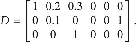
We took s = 10 and N = 128. The output Z was corrupted by white noise similar to that in the previous subsection and the signal was denoised by a db4 multiwavelet. The results obtained for the coefficient matrix A _d are shown in Figure 1. The true and identified eigenvalues of A _d are shown in Table 1.

Table 1:

True and identified eigenvalues of A _d .

True eigenvalues of A d	Identified eigenvalues of A d
0.4565 ± 0.8859i	0.4605 ± 0.8908i
0.7734 ± 0.6314i	0.7772 ± 0.6328i
0.9742 ± 0.2236i	0.9712 ± 0.2176i

One important feature of using wavelet denoising is that the system order is more easily identified. The singular values associated with the Hankel matrix Z_{0, s,N} of Section 4.2 are shown in Figure 2. Clearly, the system order is at least 5 and since it is anticipated that the order should be even, we should choose the order of the system as 6.

Figure 2:

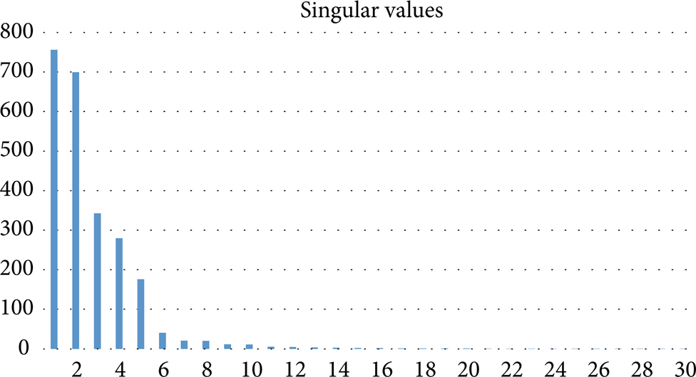
The singular values of Z_{0, s,N}.

5.3. Stochastic Subspace Identification

In this subsection, we combine numerical experiments on stochastic subspace identification and finite difference approximations to illustrate our comments in Section 4.5. In our simulation example, we obtained the discrete state-space model by applying an implicit finite difference scheme with θ = 1/2, which resulted in the following discrete state equation:

$X\left(t+\mathrm{1}\right)=\widehat{A}X\left(t\right)+w\left(t\right),$

(63)

with $\widehat{A}={(I-(\mathrm{\Delta }t/2)A)}^{-\mathrm{1}}(I+(\mathrm{\Delta }t/2)A)$ . The noise w(t) is introduced here to account for the truncation and round-off errors that result from the finite difference discretization. The system now consists of (63) and (40) with D = I.

200 Monte-Carlo simulations for the 6-dimensional structure were performed, which implement the purely stochastic subspace identification algorithm N4SID. We used the same initial conditions and 2000 measured output data. To illustrate our discussion in Section 4.5, we ran the program with various step sizes and compared the maximum true versus estimated eigenvalues of Â. The results are listed in Table 2.

Table 2:

Modal values identification using Kalman filter.

Δt	Maximum eigenvalue of Â	Maximum estimated eigenvalue of Â	% error
0.01	0.9958	—	—
0.055	0.9769	0.9050 + 0.1862i	20%
0.5	0.9769	0.9654	1%

The program did not produce meaningful results for values of Δt less than 0.055. The time duration of the recorded output for Δt = 0.5 is 1000.

5.4. An Experimental Demonstration

The developed output-only wavelet denoising identification technique is applied to a real signal. In this context, the multidisk multibearing rotor system, shown in Figure 3, with stainless steel shaft of 1 cm diameter and driven by a speed-controlled DC motor of maximum speed 10,000 rpm, is considered. The rest of specifications is described in [25].

Figure 3:

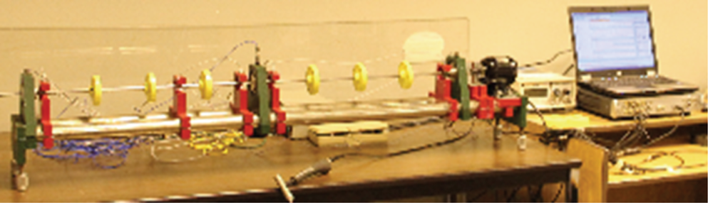
The instrumented experimental rotor system.

In this demonstration, the rotor's first three modal characteristics are identified using the developed wavelet denoising scheme of Section 3. The obtained results are compared to the values identified using experimental modal analysis (EMA) by means of LMS-Pimento 12-channel data acquisition and analysis system. The two identified results are also compared to the actual values obtained from the spectrum of a run-up test, wherein natural frequencies are recorded at resonance. The frequency spectrum of the run-up test is shown in Figure 4.

Figure 4:

Frequency spectrum of the system in Figure 2.

The rotor was speeded up gradually to a speed of 9000 rpm, thus traversing the first three natural frequencies (critical speeds), which appear as resonances. The recorded values, which represent the actual natural frequencies, are listed in the first column of Table 3. The second column of Table 3 represents the values of natural frequencies as identified by EMA. This is normally done via FRF generation, curve-fitting, peak-picking, and mode stabilization techniques, which are invoked by the modal analysis software of the LMS system in this case. It is noted that the EMA results are slightly less than the actual values because these are obtained for the stationary rotor using the roving hammer technique, while actual values are for the rotating rotor.

Table 3:

Measured and identified modal characteristics.

Measured frequencies	Identified frequency and damping (EMA)	Identified frequency and damping (wavelets)
20.258	(19.782, 0.223)	(20.782, 0.247)
64.224	(63.473, 0.152)	(63.473, 0.146)
122.413	(120.658, 0.216)	(124.658, 0.225)

Finally, to apply the developed wavelet denoising identification scheme, which is basically an output-only identification technique, we utilized the raw (noisy) signal of the measured accelerations. In this regard, direct acceleration measurements from six accelerators mounted on the three bearings; both along vertical and horizontal directions are acquired. A sample of 3072 measurements of the raw acceleration signal is shown in Figure 5, while Figure 6 shows the denoised signal, where we followed the same steps as in the simulation example of Section 4.2. In this case, the velocity and displacement signals obtained from a two-stage operational amplifier (integrator amplifier) were also denoised for any residual noise contamination. The identification scheme is then applied according to (40) to identify the system matrices. The solution of the associated eigenvalue problem results in the modal frequencies and modal shapes. The third column of Table 3 displays the calculated frequencies and modal damping as obtained by the current method. We may further examine the identified mode shapes. Figures 7 and 8 display the first two bending mode shapes, which are obtained using experimental modal analysis (EMA). In order to hold a comparison with those obtained using the current scheme, the planar plots of the normalized modes are obtained and displayed in Figures 9 and 10. The comparison shows a close agreement with EMA identified values.

Figure 5:

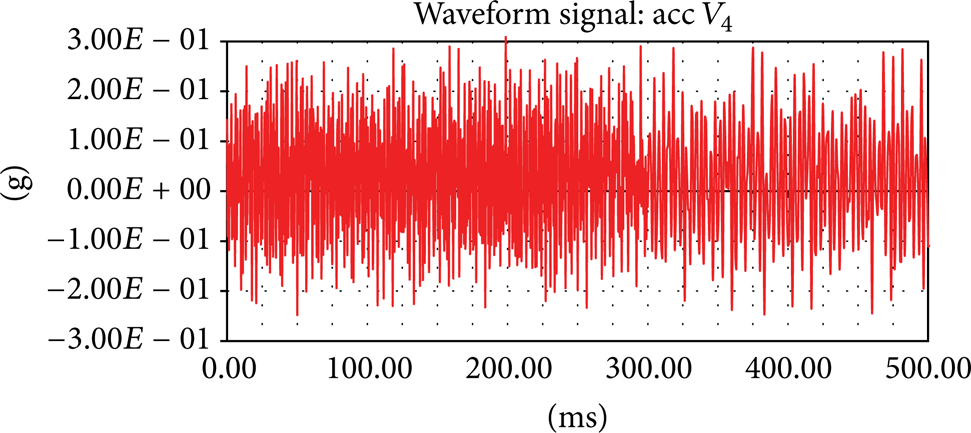
Measured acceleration signal (with noise).

Figure 6:

Denoised acceleration signal (using db4).

Figure 7:

The first bending mode.

Figure 8:

The second bending mode.

Figure 9:

The first mode shape.

Figure 10:

The second mode shape.

Although only six measurements points were utilized, the results show that the developed technique results are in good agreement with the actual values. In addition, the developed technique avoids the difficulties associated with curve-fitting and peak-picking techniques associated with FRF-based modal identification techniques. It is well oriented to time domain identification, while being based on output-only signals, thus lending itself to important applications where identifications are required for systems subjected to unknown ambient excitations. This later feature is crucial to several important applications that involve structural health monitoring and operational modal analysis.

6. Conclusions

An output-only identification scheme to estimate the system parameters of a multidimensional system from a record of noisy output measurements by using a multiwavelet denoising technique is developed. In the process, we extended the wavelet denoising methods to multiwavelet denoising. After the noise has been removed from the output records by wavelet methods, either full model identification or deterministic subspace identification could be performed. In the former case, full information on the system such as modal values and shapes becomes available by postprocessing. In the latter case, observable modal values of the system as well as modal shapes at the sensor locations can be extracted from the identified parameters. Additionally, we discussed the requirements on the measuring devices to be compatible with wavelet transforms of a particular type. The validity and merit of the developed scheme are illustrated by examples of numerically simulated and experimentally measured signals, including comparisons with stochastic identification methods. It was found out that the use of multiwavelet denoising enables us to use the more efficient and more accurate deterministic identification techniques. In particular it greatly improves the decision-making regarding the order of the system. These findings were confirmed by a simulation example as well as experimental data. In addition, the developed method avoids the difficulties associated with curve-fitting and peak-picking techniques associated with FRF-based modal identification techniques. It is well oriented to time domain identification, while being based on output-only signals, thus lending itself to important applications where identification is required for systems subjected to unknown ambient excitations. This later feature is crucial to several important applications that involve structural health monitoring and operational modal analysis.

Conflict of Interests

The authors declare that there is no conflict of interests regarding the publication of this paper.