Sage Journals: Discover world-class research

Abstract

Process monitoring and modelling can contribute to fostering the industrial relevance of additive manufacturing. Process related temperature gradients and thermal inhomogeneities cause residual stresses, and distortions and influence the microstructure. Variations in wall thickness can cause heat accumulations. These occur predominantly in filigree part areas and can be detected by utilizing off-axis thermographic monitoring during the manufacturing process. In addition, numerical simulation models on the scale of whole parts can enable an analysis of temperature fields upstream to the build process. In a microscale domain, modelling of several exposed single hatches allows temperature investigations at a high spatial and temporal resolution. Within this paper, FEM-based micro- and macroscale modelling approaches as well as an experimental setup for thermographic monitoring are introduced. By discussing and comparing experimental data with simulation results in terms of temperature distributions both the potential of numerical approaches and the complexity of determining suitable computation time efficient process models are demonstrated. This paper contributes to the vision of adjusting the transient temperature field during manufacturing in order to improve the resulting part's quality by simulation based process design upstream to the build process and the inline process monitoring.

1. Introduction

The laser beam melting (LBM) process is an additive manufacturing technology to produce almost fully dense metal parts from a powdery feedstock by utilizing a laser beam for the powder solidification. Today, a shift in the predominant application area of additive manufacturing processes from research laboratories to shop floors is evident [1]. Therefore, it is crucial to ensure a first-time-right process design and subsequently guarantee a reproducible and reliable quality standard. Process monitoring and modelling can foster this development by providing the possibility to deepen the process understanding and to improve the process design. This paper focuses on the simulation and experimental analysis of temperature fields, which are a key factor for process stability and part quality [2]. Therefore, temperature monitoring enables the detection of unpredicted process imperfections and proves the quality of each produced part. Microscale modelling provides insights on very short time scales and allows investigating corresponding process phenomena [3].

This paper wants to add scientific value by a combined view on the possibilities and limitations on both process monitoring and multiscale simulation. This can be useful to support process design for new materials or to calibrate thermal imaging data. Macroscale process models can support the process design by offering the possibility to analyze a part's temperature field upstream to the build job. Based on these temperature fields a thermomechanical analysis can be performed to forecast part deformations. These are mainly caused by residual stress release via the temperature gradient mechanism and are of major interest to technology users [4].

2. Materials and Methods

The solidification mechanisms in LBM are mainly influenced by the melt flow behavior and wettability and can be varied through the applied scanning strategy. Depending on the latter, the material is reheated in several temperature cycles resulting in residual stress and deformation. Firstly, adjacent scan tracks cause a certain volume to reheat at hatch frequency (approximately 250 Hz). Secondly, the division of the total cross section into multiple scan areas (island-shaped, stripe-wise, etc.) results in additional thermal cycles for volume regions that are located close to the scan area boundaries; compare zoomed view in Figure 1.

Figure 1:

Investigated levels of detail.

Last, the weld penetration depth is considerably larger than the nominal layer thickness which causes a remelting and reheating of already solidified part regions. Within this paper, a comparison of simulation results with data gathered through process monitoring is performed on the macro- as well as the microscale level.

Thereby, the performance in terms of time and spatial resolution is discussed. For this purpose microscale modelling allows investigating the process with the highest possible temporal and spatial resolution. Due to the required calculation time, this simulation approach is limited to a few melt tracks only. This is caused by the fact that a large amount of solution steps is necessary to realize the intended micrometer and microsecond resolution. By utilizing abstraction methods, for example, the heat input, macroscale modelling allows investigating the whole part's thermal and subsequently structural behavior resulting from the build-up process. This leads to a decreasing number of solution steps compared to microscale modelling. The achievable resolution is in the order of magnitude of millimeters and milliseconds. Process monitoring is performed inline to the process using thermal imaging and can provide a complete part inspection at a timescale of milliseconds. The investigated material within this paper is the nickel-base alloy Inconel 718, which is commonly used in turbo machinery production. The experimental and numerical methods are introduced below.

2.1. Macroscale Simulation

The macroscale approach is used for the simulation of the additive manufacturing process of complete parts. For an acceptable computation time, several simplifications are necessary [4 –8]. For a part-based simulation of the LBM process four fields of modelling can be identified [9, 10]: geometry, material, heat input, and ambient influences. Figure 2 illustrates how the geometry (first row) and the heat input modelling (second row) are carried out within this paper.

Figure 2:

Multistep procedure of geometry and heat input modeling.

As data base, a sliced representation of the part's geometry (CLI-file) is used which comprises information (point clouds) about laser scan vectors (both polylines for creating the part's contours and hatches to fill them) as well as all corresponding laser power values and scan velocities.

For the geometry modelling, the point cloud is imported to a FEA tool (ANSYS) as key points (2) after extracting the part contour (polylines) (1). Subsequently, lines are generated (3) to connect the key points. Closed vector contours are then converted to areas (4). Afterwards, the 2D-part description is extruded (5) according to the height of the present layer or layer compound (multiple layers grouped as one layer). By repeating the described procedure layer by layer or layer compound-wise the part's geometry is fully imported and a mesh which exhibits nodes on specific height levels is generated.

The heat input is modelled by prescribing a material specific temperature load to scan areas. Figure 2 (second row) illustrates the general principle of deriving scan areas from machine data. In Step 1, the whole scan vector information, hatches, and contour vectors (polylines), as transferred to the additive manufacturing machine, are shown. Steps 2 to 5 illustrate an abstraction of all scan vectors resulting in 4 load steps with a constant accumulated length of scan vectors proportional to the total length [10]. In the sense of this method, the most abstract option is to utilize only one single heat impulse to the total part cross section (solidus temperature constraint on the topmost layer). This was found to be a calculation time efficient modelling technique for the beam material interaction in order to analyze the resulting temperature field of a part to be built, but it is limited to properly model the different thermal cycles within one layer perpendicular to the build direction [8, 11].

The materials strength behavior is modelled by a multipoint linear kinematic hardening model [10].

2.2. Microscale Simulation

Several simulation approaches for laser material processing consider fluid-dynamic effects occurring in the heat affected zone [12 –14]. In this sense, electron beam melting and laser beam melting are specifically investigated in [15 –17]. Concerning this work, only conduction is considered as heat transportation mechanism within the microscale simulation model. Hence, transportation of heat energy caused by mass flow (e.g., fluid dynamics in the melt pool) is not taken into account in order to reduce calculation time.

The thermophysical properties of Inconel 718 are given in [18]. Temperature-dependent values for the absorptivity of Inconel 718 at the wavelength of Nd:YAG-laser (1.06 µm) can be found in [19]. For simplification and improvement of the convergence behavior a constant absorptivity value of 0.35 is assumed. In order to take the heat removal caused by evaporation into account, the temperature in the simulation approach is limited by the evaporation temperature of nickel (about 2915°C). The powder is modelled by a continuum approximation which means that there are no single powder particles but a solid with adapted properties [4]. Melting and solidification mechanisms of the powder bed elements are taken into account depending on their temperatures. When the temperature level reaches the solidus temperature the properties of these elements are changed to those of solid material.

For microscale modelling a heat source with a normally distributed intensity is applied. The beam properties for the investigated additive manufacturing system EOS M 270 can be found in [20]. The interaction between laser radiation and solid material is modelled by an area-related heat flux density obtained through multiplying the absorptivity by the intensity distribution [21]. Compared to solid material, the effective absorptivity of the powder domain is increased due to multiple reflections of the laser beam at the surface of the powder particles [22]. For considering the increased effective optical penetration depth a volume-related heat source is applied to the powder continuum. Here, the heat source is modelled in terms of heat flux density q_p (W/m³), which exponentially decays with powder depth z:

q_{p} (r, z) = \frac{a_{p}}{d} \exp [- \frac{z}{d}] \frac{2 P}{π w^{2}} \exp [- 2 \frac{r^{2}}{w^{2}}] .

(1)

The optical penetration depth d of the powder material is 20 µm according to [22]; the powder absorptivity a_p is assumed to be 0.6. Furthermore, P is the laser power and w denotes the 86% beam radius. The investigated process zone (500 µm × 500 µm × 60 µm) is meshed with uniform cubic elements with an edge length of 8 µm. The thickness of the powder layer is 40 µm. For modelling the underlying and already solidified regions a large block meshed with coarse tetrahedral elements is used; compare Figure 3.

Figure 3:

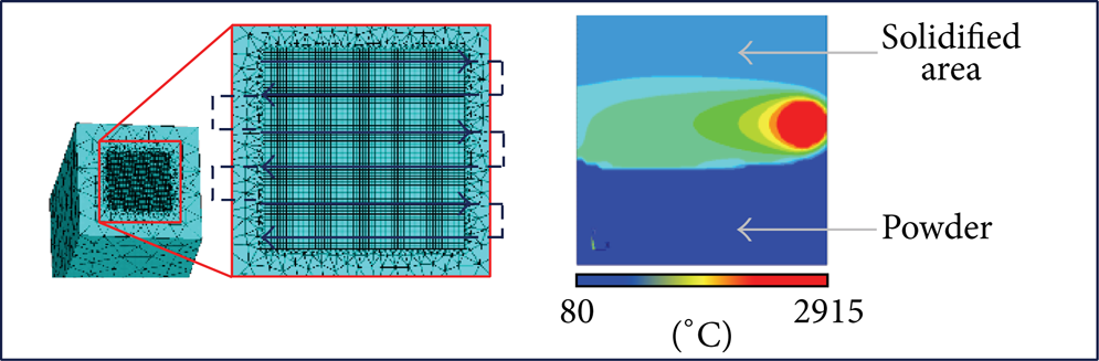
Approach for the microscale model.

2.3. Monitoring and Quality Methods

Approaches for measuring of quality-related variables (e.g., temperature, melt pool size, etc.) can be divided into coaxial setups, which are sensing the process emissions directly at the current beam position [23, 24], and off-axis setups, which usually monitor the complete build substrate at a time. In [25] the feasibility of layer-wise off-axis process monitoring based on a microbolometer IR-camera is shown and the setup used is presented. Deviations in the laser melting process, occurring at a timescale of several tens of milliseconds, can be detected by evaluating properties of the heat affected zone under idealized conditions. The typical response time for microbolometer cameras in the order of 8 ms limits the maximum frame rate to approximately 50 Hz. Furthermore, the pixel resolution of 250 µm causes spatial averaging over multiple single scan tracks (width: approximately 100 µm). Therefore, the peak temperatures cannot be determined reliably. This monitoring approach focuses on the spatially resolved analysis of the cool down behavior of a complete part section. An IR-detector (spectral range of 8 µm to 14 µm) is used to measure the associated temperature interval (melt temperature to room temperature). To derive the absolute temperature from IR measurements an effective emissivity of 0.2 is assumed, which is based on experiments that account for LBM-characteristic surface structure and the considered temperature range.

3. Results and Discussion

3.1. Macroscale Level

Based on the experimental and numerical setups described above, the temperature distributions are investigated for a blade geometry in aero engine applications. Furthermore, the thermal measurements are used to evaluate the accuracy of modelling approaches for the exposure strategy. Figure 4 shows the test specimen utilized for the macroscale investigations.

Figure 4:

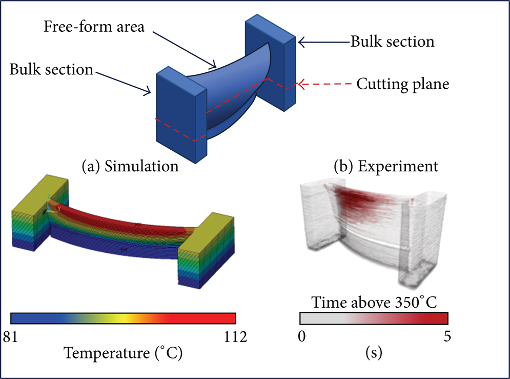
Turbine blade for macroscale investigations: simulation (a) and experimental (b) results for a cutting plane located at one-third of the part's height.

In the bottom right part of Figure 4 an experimental result illustrating the time over a specified temperature limit (350°C) is shown. On the left, the simulation result of a modelled cool down step is illustrated (based on one single heat impulse to the complete part layer for modelling the heat input to the layer compound, cf Figure 2). It can be derived that both the experimental (b) and numerical results (a) exhibit significant differences in temperature distribution perpendicular to the build direction. The difference in cooling behavior as shown in Figure 4 is due to the overhanging structure on the left side of the free-form area which features an inferior heat removal. This result is analysed in terms of element temperatures of monitoring points within the bulk and filigree free-form area of the turbine blade; compare Figure 5.

Figure 5:

Simulated temperature curves for monitoring points within the bulk and free-formed section of layer compound 20 (numerical result).

The plotted element temperatures are averaged over four nodes on the top surface of the 20th layer compound (build height: 5 mm) for both a monitoring point in the center of the bulk section and one in the free-formed area. In compliance with Figure 4(b), it can be seen that the time over 350 degrees of Celsius is higher within the filigree free-formed area compared to the massive bulk area. The reason for the temperature differences illustrated in Figures 4 and 5 is the heat transportation in reverse build direction. It is increased within the massive part regions (bulk section) compared to the free-formed section. In addition, the cool down rate for the bulk area is larger than for the filigree free-formed section. In laser beam melting, different cool down rates can influence the microstructure of parts [26]. Hence, by homogenization of the cool down behavior, the resulting microstructure could become more predictable. In addition residual stresses and deformations caused by the temperature gradient mechanism perpendicular to the build direction could be reduced.

Recapitulating, by utilizing a macroscale model to support process design, heat accumulations in, for example, free-formed part areas can be detected and could subsequently be avoided by adjusting laser power or scan velocity. For an economically efficient process design, the described simulation of the build-up process should be completed within a short period of time compared to the actual build time. To compensate for inaccuracies and to ensure part quality, process monitoring is performed to back up simulation results and to identify necessary refinements of modelling approaches.

In contrast to the numerical solution in Figure 4, a more detailed macroscale simulation approach was utilized to gather the results shown in Figure 5. Here, the heat input was modelled by accumulating the scan vectors (cf. Figure 2) to 10 scan areas which were applied with a temperature load of 1250°C for a load time corresponding to the scanning velocity (following [11]). On the one hand, the result accuracy should be increased through this measure because the thermal cycling of the elements due to the hatching of the laser (cf. Section 2) can be modelled more accurately. On the other hand, the calculation time for the thermal solution of 20 layers increased from 16 minutes to 215 minutes. The effect of this modelling approach on the result accuracy can be investigated in Figure 6 which shows the temperature curve of three elements within the first scan area (top right corner) of layer compound 20.

Figure 6:

Temperature curve layer compound 20 (time scale adjusted) for 3 monitoring points within a load area in the top right corner (numerical result).

Thereby, elements on the left end of the scan area, in the center, and on the right end were chosen. Due to the fact that the spatial resolution is limited by the element size, the elements on the left end of the scan area were also within the selection of the second scan area which explains the peaks at about 1.4 s. Hence, this approach enables the modelling of additional temperature cycles for neighboring scan areas as discussed in Section 2. Furthermore, the approach is capable of modelling the contour exposure that completes the solidification of the current part cross section (peak at 2.5 s in Figure 6). Through heat conduction an increase in temperature can also be detected for the elements in the center and on the left at 2.5 s. It can also be seen that the general temperature level in Figure 6 is above approximately 190°C once the solidification of layer compound 20 is started (0.55 s), although the chosen preheat temperature is 80°C. This effect is caused by heat accumulation due to a restricted influence of the base plate on the heat conduction rate between part and base plate. Figure 7(b) shows a measured temperature evolution at different points of interest for a corresponding part section during the process. The measured temperature level can be compared to the model (cf. Figure 6).

Figure 7:

Experimental results obtained by thermography. Layer-integrated image showing time above 500°C level (a). Temperature evolution for different subareas at measurement points (b).

To enable a straightforward identification of hot spots, Figure 7(a) displays the geometrically mapped data for a characteristic layer-wise cool down time (derived from the total time above a certain temperature). Both the figure and the chart in Figure 7 describe the same physical background of delayed heat dissipation and can be used as a quality indicator. Furthermore, it can be concluded that the temperature evolution varies significantly between the first and second scan areas. After exposing the first scan area, the overall temperature in its vicinity increases and causes a slower cool down of the second scan area. In accordance with the numerically investigated temperature curves shown in Figure 5 the time above a fixed temperature (e.g., 350°C) is increased for the monitoring point within the free-formed area.

3.2. Microscale Level

The microscale model is intended to simulate the subsequent exposure of single tracks only. Compared to the macroscopic, part-based level, the temperature distribution and its temporal evolution can be investigated with an increased temporal and spatial resolution (micrometers and microseconds). A comparison of measurement data is only reasonable at the level of multiple scan tracks, taking into account the spatial and temporal averaging caused by the inertia of the measurement setup. To compare the numerical results of the microscale simulation with experimental data from thermography a modelled volume region of 250 µm × 250 µm × 40 µm is investigated by averaging corresponding nodal temperatures (cf. Section 2). This equals the pixel size of the measurement setup: compare Figure 8.

Figure 8:

Bolometer measurement of >40 hatches for fixed region of interest (b) compared with macroscale simulation results ((c), cf. Figure 5) and microscale simulation of several single hatches (a).

As introduced in Section 2 of this paper, hatching takes place on microscale level (10 µm, 10 µs) and states the main influence on temperature evolution through reheating (cf. Figure 8). Because of spatial (250 µm) and temporal (20 ms) resolution limits in the bolometric measurement setup, the layer-wise monitoring approach is mainly suitable for investigating the cooling behavior and long term temperature field evolution; compare Section 3.1. Due to spatial averaging the cooling behavior for single tracks is superimposed by the current temperature of its vicinity, resulting in a low frequency temperature rise as the heat source passes by.

To compare the simulation results—from both the micro- and the macroscale models—with the experimental results the width of the temperature curves and the cooling rates are investigated. Hereby, the width of a temperature curve is defined by the time; the temperature of an observed area region is above a fixed value of 500°C and cooling rate means the change with time of the temperature curve. The microscale model exhibits the fastest cooling rates compared to both the macroscale simulation and the experiments. Concerning the microscale model, the maximum cooling rate is −378.49°C/ms and the temperature peak width is 1.98 ms (Figure 8(a), first peak). As stated before, the thermography camera is not able to resolve the repeated heating cycles caused by neighbored hatches due to the inertia of the experimental setup. The maximum cooling rate measured with the bolometer is −1.74°C/ms and the width of the temperature curve is in this case 60.80 ms. These values broadly correspond with the results obtained from the macroscale simulation where a maximum cooling rate of −4.83°C/ms and a width of the temperature peak of 20.02 ms are observed.

4. Conclusions

Macroscale process modelling can be utilized to investigate the temperature field during the build process. Therefore, necessary adjustments to achieve a homogeneous temperature field perpendicular to the build direction can be identified upstream to the build process. As a result, the process design could be improved. In contrast to the state of the art, this would lead to an adjustment of process parameters within a part (e.g., increased scan velocity in the free-formed (cf. Figure 4) part area) in dependence on the wall thickness. To ensure the part quality and document the homogenized temperature field, the build-up process should be monitored, for example, by thermography.

On the macroscale level, abstract modelling approaches need to be applied for the virtual process design in order to gather numerical results within a computing time which is less than the build time of the part. To evaluate the accuracy of element temperatures (cf. Figures 5 and 8) process monitoring results should be considered. Thereby, the limitations of abstractions can be derived and users can decide whether they want to apply maximal calculation time efficient approaches or rather need increased result accuracy.

Process monitoring at the level of microseconds states an interconnection between microscale and macroscale modelling in the following way. Macroscale simulation cannot investigate random process irregularities on the part-based level but allows the prediction of possible systematic errors and deterioration of part quality and part deformations. Microscale modelling cannot handle full featured part geometries but allows a detailed understanding of realistic temperature cycles during hatching. Compared to macroscale modelling, the layer-wise process monitoring approach is capable of detecting geometry-dependent systematic and especially random irregularities during the manufacturing process by investigating the cool down behavior as the heat source passes by.

Future work comprises an integration of process monitoring and modelling. On a macroscale level, results from thermal imaging can be imported to the simulation system in order to perform a simulation of the resulting part's structural behavior, in particular, the resulting residual stress state which is cost intensive to measure. Furthermore, temperature profiles gathered through thermal imaging can contribute to the improvement of suitable abstraction methods for heat input modelling. On a microscale level, simulation results are of use for the calibration of measurement equipment and also for validating abstraction methods for macroscale modelling in terms of, for example, the energy intensity.

In addition, future work should focus on an improvement of both the simulation models and the experimental setup for thermal imaging. For an improved comparison of the microscale simulation model and the thermography results, an increase of temporal and spatial resolution compared to the setup used within this work is necessary.

Conflict of Interests

The authors declare that there is no conflict of interests regarding the publication of this paper.

Footnotes

Acknowledgment

The research leading to these results has received funding from the European Union's Seventh Framework Programme (FP7/2007–2013) for the Clean Sky Joint Technology Initiative under Grant agreement no. 287087.

References

Wohlers

, Wohlers Report 2012: Additive Manufacturing and 3D Printing State of the Industry—Annual Worldwide Progress Report, 2012.

Zaeh

M. F.

and Ott

, “Investigations on heat regulation of additive manufacturing processes for metal structures,” Annals of the CIRP, vol. 60, no. 1, pp. 259–262, 2011.

Roberts

I. A.

Wang

C. J.

Esterlein

Stanford

, and Mynors

D. J.

, “A three-dimensional finite element analysis of the temperature field during laser melting of metal powders in additive layer manufacturing,” International Journal of Machine Tools and Manufacture, vol. 49, no. 12–13, pp. 916–923, 2009.

Zaeh

M. F.

and Branner

, “Investigations on residual stresses and deformations in selective laser melting,” Production Engineering, vol. 4, no. 1, pp. 35–45, 2010.

Seidel

Zaeh

M. F.

Weirather

, “Simulation of the laser beam melting process—an approach for an efficient geometry modelling of complex lightweight parts,” in Proceedings of the DGM LightMAT, Deutsche Gesellschaft für Materialkunde e.V., 2013.

Krol

T. A.

Westhaeuser

Zaeh

M. F.

Schilp

, and Groth

, “Development of a simulation-based process chain—strategy for different levels of detail for the preprocessing definitions,” in ASIM 2011-21. Symposium Simulationstechnik, Boedi

and Maurer

, Eds., Winterthur, Del, USA, September 2011.

Keller

Neugebauer

, and Ploshikhin

, “Thermo-mechanical simulation of ALM of titanium aerospace structures,” in Proceedings DGM LightMAT 2013, e. V. Deutsche Gesellschaft für Materialkunde, Ed., 2013.

Krol

T. A.

Seidel

, and Zaeh

M. F.

, “Prioritization of process parameters for an efficient optimisation of additive manufacturing by means of a finite element method,” in Proceedings of the 8th CIRP Conference on Intelligent Computation in Manufacturing Engineering vol. 12, pp. 169–174, 2013.

Seidel

Krol

T. A.

Schilp

Zaeh

M. F.

, and Groth

, “Ansätze zur rechenzeiteffizienten Struktursimulation additiv gefertigter, filigraner Bauteile,” in Proceedings of the ANSYS Conference & 30th CADFEM Users' Meeting, CADFEM GmbH, Ed., Kassel, Germany, 2012.

10.

Seidel

Zaeh

M. F.

Weirather

Krol

T. A.

Schilp

, and Schmid

, “Prozessnahe Modellierung des Materialverhaltens beim Laserstrahlschmelzen als Grundlage für die Ergebnisgenauigkeit hinsichtlich der Bauteilmaßhaltigkeit und des Eigenspannungszustandes,” in Proceedings of the ANSYS Conference & 31th CADFEM Users' Meeting, CADFEM GmbH, Mannheim, Germany, 2013.

11.

Seidel

Zaeh

M. F.

Wunderer

Weirather

Krol

T. A.

, and Ott

, “Simulation of the laser beam melting process approaches for an efficient modelling of the beam-material interaction,” in Proceedings of the 8th International Conference on Digital Enterprise Technology, Fraunhofer Institute for Industrial Engineering (IAO), Stuttgart, Germany, 2014.

12.

Otto

and Schmidt

, “Towards a universal numerical simulation model for laser material processing,” Physics Procedia, vol. 5, pp. 35–46, 2010.

13.

Otto

Koch

Leitz

K.-H.

, and Schmidt

, “Numerical simulations—a versatile approach for better understanding dynamics in laser material processing,” Physics Procedia, vol. 12, pp. 11–20, 2011.

14.

Otto

Koch

, and Vazquez

R. G.

, “Multiphysical simulation of laser material processing,” Physics Procedia, vol. 39, pp. 843–852, 2012.

15.

Körner

Attar

, and Heinl

, “Mesoscopic simulation of selective beam melting processes,” Journal of Materials Processing Technology, vol. 211, no. 6, pp. 978–987, 2011.

16.

Attar

and Körner

, “Lattice Boltzmann model for thermal free surface flows with liquid-solid phase transition,” International Journal of Heat and Fluid Flow, vol. 32, no. 1, pp. 156–163, 2011.

17.

Guertler

F.-J.

Karg

Leitz

K.-H.

, and Schmidt

, “Simulation of laser beam melting of steel powders using the three-dimensional volume of fluid method,” Physics Procedia, vol. 41, pp. 874–879, 2013.

18.

Pottlacher

Hosaeus

Wilthan

Kaschnitz

, and Seifter

, “Thermophysikalische Eigenschaften von festem und flüssigem Inconel 718,” Thermochimica Acta, vol. 382, pp. 255–267, 2002.

19.

Sainte-Catherine

Jeandin

Kechmair

Ricaud

J.-P.

, and Sabatier

, “Study of dynamic absorptivity at 10.6 μm (CO₂) and 1.06 μm (Nd-YAG) wavelengths as a function of temperature,” Journal de Physique, vol. 1, pp. C7-151–C7-157, 1991.

20.

Krauss

and Zaeh

M. F.

, “Investigations on manufacturability and process reliability of selective laser melting,” Physics Procedia, vol. 41, pp. 815–822, 2013.

21.

Hussein

Hao

Yan

, and Everson

, “Finite element simulation of the temperature and stress fields in single layers built without-support in selective laser melting,” Materials and Design, vol. 52, pp. 638–647, 2013.

22.

Fischer

Romano

Weber

H. P.

Karapatis

N. P.

Boillat

, and Glardon

, “Sintering of commercially pure titanium powder with a Nd:YAG laser source,” Acta Materialia, vol. 51, no. 6, pp. 1651–1662, 2003.

23.

Craeghs

Clijsters

Yasa

, and Kruth

J.-P.

, “Online quality control of selective laser melting,” in Proceedings of the Solid Freeform Fabrication, University of Texas at Austin, 2011.

24.

Craeghs

Bechmann

Berumen

, and Kruth

J.-P.

, “Feedback control of Layerwise Laser Melting using optical sensors,” Physics Procedia, vol. 5, pp. 505–514, 2010.

25.

Krauss

Eschey

, and Zaeh

M. F.

, “Thermography for monitoring the selective laser melting process,” in Proceedings of Solid Freeform Fabrication, University of Texas, Austin, Tex, USA, 2012.

26.

Thijs

Verhaeghe

Craeghs

Humbeeck

J. V.

, and Kruth

, “A study of the microstructural evolution during selective laser melting of Ti-6Al-4V,” Acta Materialia, vol. 58, no. 9, pp. 3303–3312, 2010.

Investigations on Temperature Fields during Laser Beam Melting by Means of Process Monitoring and Multiscale Process Modelling

Abstract

1. Introduction

2. Materials and Methods

2.1. Macroscale Simulation

2.2. Microscale Simulation

2.3. Monitoring and Quality Methods

3. Results and Discussion

3.1. Macroscale Level

3.2. Microscale Level

4. Conclusions

Conflict of Interests

Footnotes

Acknowledgment

References