Sage Journals: Discover world-class research

Abstract

In this work, a journal bearing optimization process has been developed and is divided into two stages. Each one has a set of decision variables and custom objectives aggregating performances with a weighting strategy. The performance functions used are an artificial neural network, trained with Reynolds equation solutions, and a CFD simulation of the bearings carried out with commercial software. The results show the capabilities of the algorithm to design and optimize journal bearings by reducing both power loss and mass flow with respect to ones designed with traditional methods, as well as by minimizing the maximum and average temperature.

1. Introduction

While today's automotive facilities, especially in the field of internal combustion engines, are relatively efficient, significant opportunities remain to reduce power losses and fuel consumption. One possible way to achieve this goal is to work on the efficiency of vehicular lubrication systems as well as on other aspects like weight, complexity, and reliability. Recent investigations estimate that 25% of the total mechanical power losses in terrestrial vehicles are due to journal bearings [1], a fact which focuses our attention on them because of the great benefits that the optimization of these components would produce. Furthermore, optimizing the whole lubrication system is not practically possible and, in some cases, inconvenient.

The problem of hydrodynamic journal bearings (HJB) optimization is related to three fundamental goals: to design a fast and precise function to calculate the performance of the bearing, devise the optimization objectives, and choose a rapid and globally convergent technique to find the global minimum or maximum of the aforementioned objectives. Hence, the optimal choice of parameters for the design of journal bearings is a multivariable and multiobjective problem. The aim of this work is not only to choose an optimal set of decision variables but also to provide a realistic solution where temperature, pressure, and film thickness are controlled and where the quality of the process can be evaluated objectively.

Numerous techniques have been developed to predict the performances of HJB and can be divided into four categories: approximated methods [2 –4], rigorous solution of the Reynolds equation [5 –7], curve fitting, and CFD solution with commercial software. The first group is based on the fact that the pressure profile and solution of the Reynolds equation of lubrication can be imitated using the proper combination of functions whose variables are eccentricity and length to diameter ratio. These techniques are reliable only in a specific range of ε (eccentricity ratio) and λ (length to diameter ratio) and cannot take into account misalignment of the shaft and lubricant inlet conditions. Furthermore, in order to iterate the value of the viscosity, some approximated methods are coupled with approximated functions to predict the shaft temperature and the average lubricant temperature. However, material properties are not included in the calculations [8].

Carrying out the Reynolds equation solution with finite difference or finite elements is one of the most accurate ways to solve the pressure field of an HJB. However, in terms of time and programming skills, these methods can be expensive, especially in the case where the Reynolds equation is coupled with the energy equation and heat conduction equation to solve the temperature field. In the case where the viscosity is the function of other variables, such as pressure and shear stress, other coupled functions have to be solved. If cavitation is considered or dynamic loaded HJB are analysed, the Reynolds equation must be modified. Hirani and Biswas [9] developed a modified Reynolds equation to solve the cavitation problem. Another technique that can be classified as rigorous is the exact analytical solution of the Reynolds equation carried out by Chasalevris and Sfyris in [10]. Here, the exact analytical solution of the Reynolds partial differential equation is presented. The results are validated using numerical methods (FEM and finite difference) and approximated solutions.

Zengeya and Gadala [11] developed functions to predict mass flow and power loss. The proposed equations were obtained by fitting both solutions of the Reynolds equation that were obtained with FEM techniques and literature data. Because of their form, no integrations are needed to calculate the performances of HJB and numerous critical design variables are taken into account. Artificial neural networks (ANN) studied by Ghorbanian et al. in [12] is another example of a curve fitting solution where numerous examples of the exact solution have been calculated with finite differences and are fitted by a network of neurons in order to evaluate the performances of bearings for every eccentricity and geometrical dimensions.

HJB used commercial CFD tools from Gertzos et al. [13] and the results were validated with the Raimondi and Boyd charts. In [14], Bompos and Nikolakopoulos solution of HJB was analysed with magnetorheological fluids.

A suitable performance function for optimization has to be fast and universal. In terms of calculation time, the optimization algorithms simultaneously calculate the objectives of numerous subjects; thus, the optimization time is dramatically affected by the performance calculation time. The second aspect, universality, is the ability of the function to be able to calculate the performances of a bearing with any combination of decision variables and without design limitations. In this paper, the performance functions are an ANN trained with Reynolds equation's solutions.

In terms of the optimization process and the objective design, Ghorbanian et al. [12] use genetic algorithms to minimize oil consumption and power loss, which are conflicting aims. Hirani and Suh [15] use a nonsorted genetic algorithm (NSGA) to minimize two objectives. The first is made of the sum of nondimensional power loss and penalties and the second sums up the nondimensional mass flow and penalties of the HJB. The penalties are coefficients aggregating together maximum pressure, minimum film thickness, and temperature rise.

Zengeya and Gadala in [11] aggregate several performances using a scaling and weighting strategy. The scaling and weighting factors are arbitrarily chosen, which determine the generation of a single objective space in which the solution is found. The last relevant work in this field, made by Boedo and Eshkabilov in [16], uses the genetic algorithm technique to optimize the shape of statically loaded journal bearings.

In this work, the optimization strategies adopted for the calculation are non-Sorted Genetic Algorithm (NSGA-II) and Artificial Bee Colony Algorithm (ABC) from [17]. ABC belongs to the category of particle swarm intelligence and has never been used to solve tribological issues, nevertheless, it has already demonstrated to be an excellent optimization technique for technological problems. In [18] Sonmez uses the ABC technique to solve the multiobjective problem of scheduling generators to fulfil the demand of energy. In [19], Anandhakumar et al. used the ABC capabilities to solve the problem of diesel engine maintenance.

The optimization process is divided in two stages. During first stage, the decision variables are diameter, clearance, and length to diameter ratio. The objective functions are designed to take into account and aggregate the performances of the bearing to control some technological aspects. During the second stage, only the ABC algorithm is employed to minimize the product between the maximum and average temperature in the bearing. The decision variables are supply hole geometry, such as diameter, position, and shape, while the supply pressure is fixed. In this work, the journal bearing optimization is a minimum-minimum problem where the objective functions must be minimized.

As pointed out by Ghorbanian, the previous works use discrete decision variables, and it must be emphasized that the decision variables are not, in essence, discrete because of numerous manufacturing reasons. Also, lubricant viscosity has a strong effect on journal bearing performances; nevertheless, dynamic viscosity is not included in the list of decision variables for two main reasons: journal bearings (and in general all the components of the lubrication systems) are subsystems of other main facilities, for example, ICE or gear transmissions. This main system drives the selection of the lubricant requiring the other subsystems to adapt their features to this choice. Secondly, the viscosity of lubricants for commercial use is determined by standards (ISO, SAE). The use of viscosity as a decision variable leads to an optimization driven by oil parameters with values of dynamic viscosity and a density that is different from the lubricants used in the real practice (automotive and industry).

The method used to include the viscosity effect in the optimization is to repeat the optimization for different viscosities and create optimization maps.

This work provides a methodology to optimize the HJB in respect to a reference design which could be calculated with classical methods or by an existing bearing. The algorithms presented can also be used to design a new bearing. The reference design is used to provide a proof of the soundness of the algorithm.

2. Optimization Methodology

2.1. Optimization Strategy

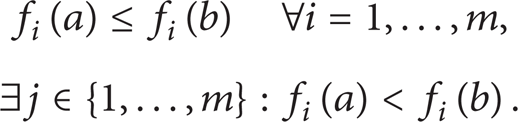
A general optimization problem is posed as follows:

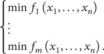
{\begin{cases} \min f_{1} (x_{1}, \dots, x_{n}) \\ ⋮ \\ \min f_{m} (x_{1}, \dots, x_{n}) . \end{cases}

(1)

Here, m is the number of objectives to be minimized and n is the number of decision variables. The aim of the optimization is to find the set of decision variables that simultaneously minimize the objectives’ functions. These objectives have to be designed to take into account numerous performances, as well as the fact that the decision variables range must be not be restrictive. Performance functions with the capability to calculate the performance of all the possible combinations of values of decision variables have been designed and a reliable and globally converged method to find the solution has been built. In this work, the optimization is divided into two stages with m₁ = 2, n₁ = 3, m₂ = 1, and n₂ = 2. The performance functions are an ANN trained with results obtained from solving with finite difference, the Reynolds equation, and the CFD solution. Finally, the optimization methods are GA and ABC.

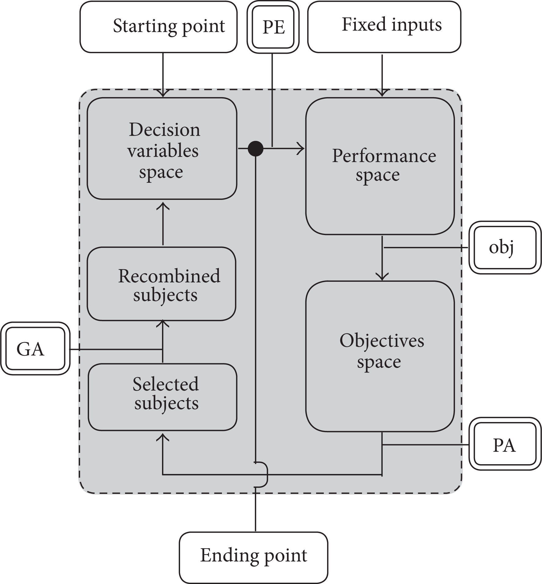
As demonstrated by Hirani and Suh in [15], not all variables have the same effect on the optimization. Some geometrical variables, regarding the inlet geometry, do not have a significant effect on performances such as power loss and mass flow. On the other hand, the inlet positioning and design can strongly influence the temperature field in terms of maximum temperature and reverse flow phenomena. Also, Singhal and Khonsari in [20] showed how the inlet pressure and viscosity (directly related to the temperature) influence the cross-coupling damping coefficients and how the inlet temperature influences the whirl threshold. These facts determine the need to split the optimization problem solution in two stages, as shown in Figure 1, with different objectives: performance functions and minimization techniques.

Figure 1:

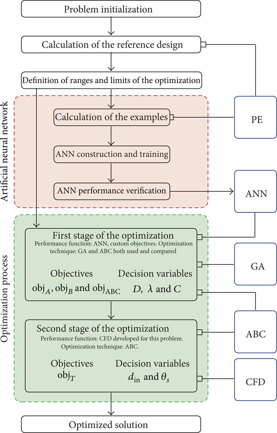
Optimization methodology scheme. PE is the performance function; ANN is the artificial neural network function. GA and ABC are the two optimization techniques and CFD is the tool used to calculate the maximum temperature (square with line: function usage; arrow with line: work flow).

2.2. Performance Calculation

The standard form for the performance function can be written as

y = p e r f o r m a n c e (x) .

(2)

In this function, y is the performance vector and x is the decision variable vector. The y vector is made of five terms: power loss, lubricant consumption, temperature rise, maximum pressure, and minimum oil film thickness. The decision variable vector is made of three terms: diameter, clearance, and length to diameter ratio. In addition, some other constant variables are inserted into the performance function, such as the rotational speed, shaft torque, lubricant properties, applied force, and material properties (all of these are constant for a given problem).

The “performance” function can be any kind of function able to calculate the HJB performances for a given set of variables. In this work, an ANN is used and is trained with the solutions of the Reynolds equation (RE). The RE is valid for finite-length HJB (0.25 ≤ λ ≤ 4) and is valid for a range of eccentricities between 0.1 and 0.9. The general form of RE is [5]

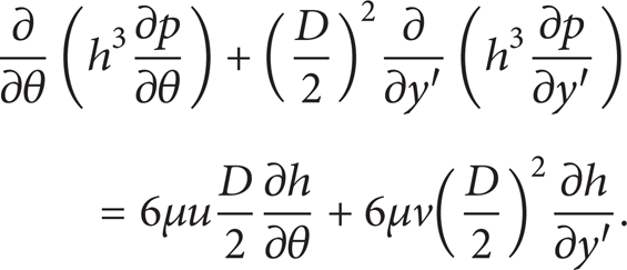
\frac{\partial}{\partial θ} (h^{3} \frac{\partial p}{\partial θ}) + {(\frac{D}{2})}^{2} \frac{\partial}{\partial y^{'}} (h^{3} \frac{\partial p}{\partial y^{'}}) = 6 μ u \frac{D}{2} \frac{\partial h}{\partial θ} + 6 μ v {(\frac{D}{2})}^{2} \frac{\partial h}{\partial y^{'}} .

(3)

In this form, p is the pressure, D the diameter of the journal, h the film thickness, u the radial velocity, v the axial velocity (which is zero for this work), θ the angular coordinate, and y′ the axial coordinate visible in Figure 2. For this solution, the finite difference technique was employed. If the misalignment of the rotational axis on the plane z′-y′ is considerable (>0.005°), the film thickness formula is

h = C + ε C \cos (θ - θ_{0}) + \tan (γ) (y^{'} - \frac{L}{2}) \cos (θ - θ_{0}),

(4)

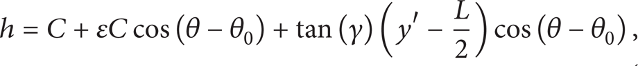
where C is the clearance, L is the length of the bearing, θ₀ is the attitude angle, and γ is the misalignment angle that can be evaluated as follows (angle between the y′ axis and plane x′-y′):

γ = \frac{F L_{f}^{2}}{16 E J} .

(5)

Above, F is the force acting on the bearing, L_f is the distance between the application point of the force, and the plane z′ − y′ minus is the distance L/2. E is the elasticity modulus and J is the inertial moment of the shaft section (which is supposed to be constant). In formula (3), the u and v can be calculated as

u = (\frac{π D ω}{60}) \cos γ,

(6a)

v = (\frac{π D ω}{60}) \sin γ .

(6b)

The rotational speed is ω in rpm.

Figure 2:

Basic structure of HJB (the dimension of the clearance is magnified).

Within these conditions, the finite differences scheme must be applied as presented in [5]; otherwise, (4) can be simplified as

h = C + ε C \cos (θ - θ_{0}) .

(7)

And the RE can be expressed in terms of Vogelpohl parameters employing the dimensionless variables

h^{*} = \frac{h}{C}, θ^{*} = \frac{2 θ}{D}, y^{*} = \frac{y^{'}}{L}, p^{*} = \frac{p C^{2}}{3 u μ D} .

(8)

The Voghelpohl parameter is:

M_{v} = p^{*} h^{* 1.5} .

(9)

And the RE can be written as

\frac{\partial^{2} M_{v}}{\partial θ^{* 2}} + {(\frac{D}{2 L})}^{2} \frac{\partial^{2} M_{v}}{\partial y^{* 2}} = F_{v} M_{v} + G_{v},

(10)

where the parameters F_v and G_v for the journal bearings are

F_{v} = \frac{0.75 [{(\partial h^{*} / \partial θ^{*})}^{2} + {(D / 2 L)}^{2} {(\partial h^{*} / \partial y^{*})}^{2}]}{h^{* 2}} + \frac{1.5 [(\partial^{2} h^{*} / \partial θ^{* 2}) + {(D / 2 L)}^{2} (\partial^{2} h^{*} / \partial y^{* 2})]}{h^{*}},

(11a)

G_{v} = \frac{(\partial h^{*} / \partial θ^{*})}{h^{* 1.5}} .

(11b)

Using this simplified form, the finite difference scheme can be applied.

After the pressure profile is found, the performance is calculated as follows:

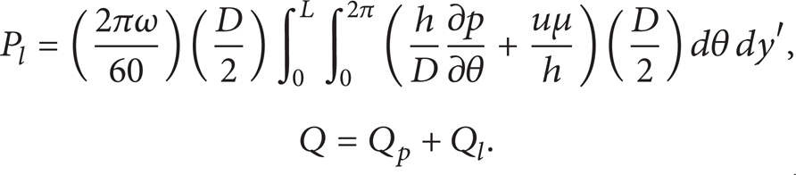
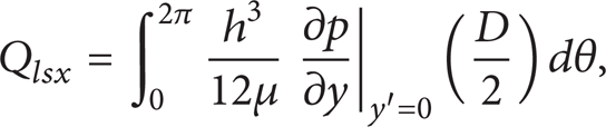
\begin{matrix} P_{l} = (\frac{2 π ω}{60}) (\frac{D}{2}) \int_{0}^{L} \int_{0}^{2 π} (\frac{h}{D} \frac{\partial p}{\partial θ} + \frac{u μ}{h}) (\frac{D}{2}) d θ d y^{'}, \\ Q = Q_{p} + Q_{l} . \end{matrix}

(12)

In this form, Q_p is the mass flow due to the pumping effect and Q_l is the mass flow side leakage that can be calculated as follows [5]:

Q_{l} = Q_{l s x} + Q_{l d x},

(13a)

Q_{l s x} = {\int_{0}^{2 π} \frac{h^{3}}{12 μ} \frac{\partial p}{\partial y} |}_{y^{'} = 0} (\frac{D}{2}) d θ,

(13b)

Q_{l d x} = {\int_{0}^{2 π} \frac{h^{3}}{12 μ} \frac{\partial p}{\partial y} |}_{y^{'} = L} (\frac{D}{2}) d θ .

(13c)

The pumped mass flow, Q_p, can be evaluated as follows:

Q_{p} = (\frac{π D ω}{120}) (A_{\max} - A_{\min}) .

(14)

In this form, A_max is the tangential area in the point of maximum film thickness and A_min the area in the location of the minimum film thickness.

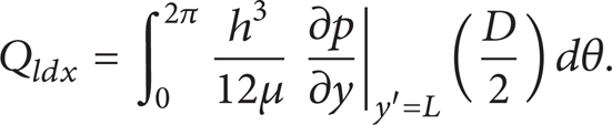
P_max is the maximum pressure of the lubricant and h_min is the minimum film thickness calculated with formula (4) or (7). The temperature rise is calculated using the approximated approach proposed by [15]

Δ T = \frac{ε F_{fric} u}{ρ_{0} C_{0} Q_{l}},

(15)

where ε is the eccentricity ratio and is used as a factor, as demonstrated in [15], that can approximate the fraction of heat flow which is dissipated by the oil flow.

The dynamic nature of the problem is well known to the authors. In fact, in numerous studies, the RE is added to the term ∂h/∂t, where t is the time. After a period of warming up, the only variable factor is the load. If the time dependency has a great effect on the performances, then it has to be considered; otherwise, the reader can calculate the equilibrium position with the equation proposed in [7]. The present analysis is limited to statically loaded journal bearings; nevertheless, the method can be used also for dynamically loaded ones.

Because the solution of the partial differential equations (PDEs) in (3) and (10) can be expensive in terms of time for the optimization process, an interactive interpolation process, like neural networks, is used.

The architecture of an ANN is fairly simple. It is made of three layers: the input layer, the hidden layers, and the output layer, all connected by synapsis. The input layer has a number of neurons that is equal to the number of input variables and the output layer as a number of neurons that is equal to the number of outputs, in this work always one. When it comes to hidden layers, both the number of layers and the number of neurons depend on the problem's complexity. To accurately predict the outputs without creating oversized networks, the number of hidden layers has to be calculated by measuring the error produced by the output neurons with respect to a reference. This procedure has been repeated since the minimum number of neurons, given the selected accuracy, was found.

Neurons are the nodes of the network grid. Their classification is based on the transfer function “f”: “sigmoid,” “linear,” and “hard limit.” In Figure 3, a typical example of a neuron is shown and in Figure 4 an example of network is shown. The output is combined with the weight vector and added to the bias vector. The weight vector is the object of the training process which is the technique used by the network to fit the function. The weights are adjusted since the predictions, compared to the example set of known results, give an acceptable error (10⁻⁴). In this work, the ANN uses the measurement of the mean sum of squares of the network errors to give a feedback for training; in fact, the network is also called feedforward neural network [21]. In this paper, the network is made of an input layer with 3 neurons, an output layer with 1 neuron, and an optimal number of hidden layers listed in Table 1 with a fixed number of 10 neurons. The transfer functions are all sigmoid due to the nonlinear nature of the results.

Table 1:

Optimum number of hidden layers.

Network	Hidden layers

annP_l	12
annQ	14
annΔT	4
ann P_max	4
ann h_min	5
anne	3

Figure 3:

The scheme shows a single neuron for scalar and vector inputs.

Figure 4:

The scheme shows a network of neurons with vector inputs. The ANN in the example is made with the P_max network. In the hidden network, every dot is neuron. The connections between neurons are shown just in one case with dashed line. The reader has to imagine that every neuron is connected with every neuron of the successive layer.

ANN is a dynamic curve-fitting tool that has the ability to generalise. This property allows the network to predict cases not coming from the training session cases. From a practical point of view, it works like a formal solver for PDEs in (3) and (10). If the training examples are homogeneously distributed among the variable ranges numerous enough, then the network can accurately predict the results of the problem. The variable space is a four-dimensional and includes three decision variables as well as the eccentricity. Every variable is divided into 9 nodal values for a total number of combinations of 9⁴ = 6561. Within these examples, 80% are used for training, 10% for test, and 10% for the validation. ANN is commonly used in numerous scientific fields and the practice suggests that is not convenient to generate a single large network to simultaneously predict several results of a function, but it is better to divide the network into little networks. These nets have specific tasks; hence, their “weight” and “bias” vectors can be obtained easily and the results can be predicted with as little amount of layers and neurons per layer without losing accuracy; the results are shown in Table 1. In this work, five ANNs have been trained for the five different outputs required to the performance function. Consider

[\begin{bmatrix} P_{l} \\ Q \\ Δ T \\ P_{\max} \\ h_{\min} \end{bmatrix}] = ann (D, λ, C) = {\begin{cases} ann P_{l} (D, λ, C) \\ ann Q (D, λ, C) \\ ann Δ T (D, λ, C) \\ ann P_{\max} (D, λ, C) \\ ann h_{\min} (D, λ, C) . \end{cases}

(16)

Another hidden neural network was developed to predict the contact between shaft and bearing. The name of the network is “anne” and is a perceptron network made of neurons with “hard limit” function. The scope of this network is to find the combinations of decision variables that cause contact between sleeve and shaft.

In addition to ensuring the quality of the solution, the critical rotational speed is calculated using the approximated approach proposed by Hashimoto as interpolation of the Routh-Hurwitz scheme:

ω_{c r} = (\sqrt{\frac{g}{C}}) (0.0584 \exp (6.99 ε^{2.07}) - 1.318 ε + 2.873) .

(17)

The accuracy of the prediction was evaluated with the comparison between the HJB characteristics plots calculated with finite difference and predicted by the ANN and is shown in Figure 5.

Figure 5:

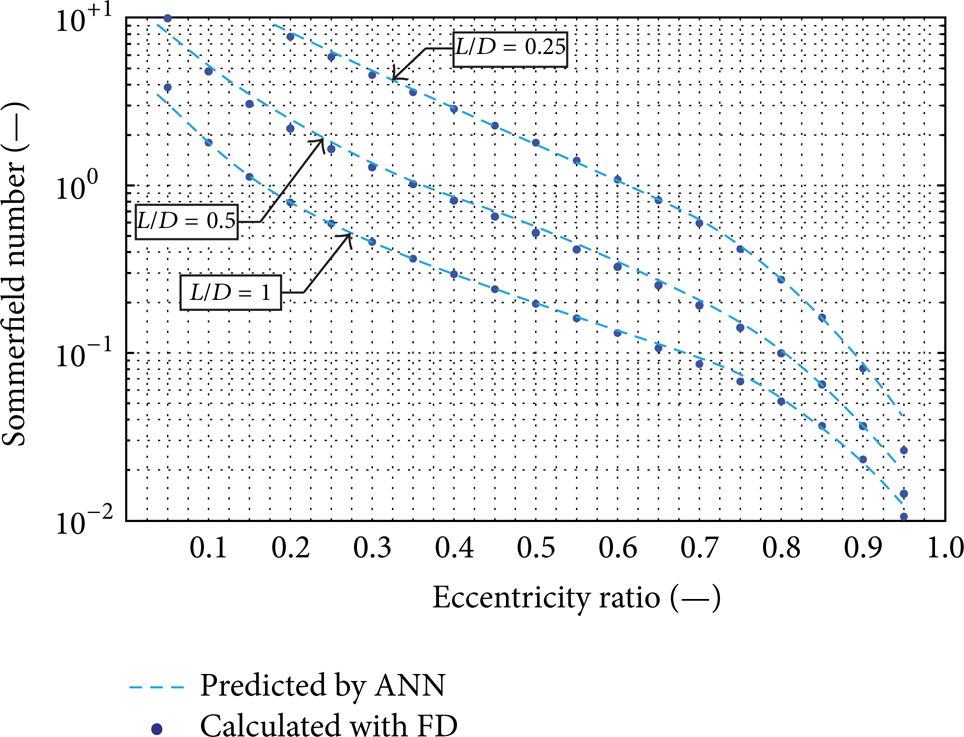
Results of the training process of the ANN.

2.3. Objective Definition

The objective functions have been designed to aggregate the performances of HJB. Optimizing a single performance is not convenient. However, some authors optimize only two objectives composed by the single performance or by a nondimensional form of it. Others in [2] chose to optimize two performances and constrain the others (temperature rise, maximum pressure, and minimum film thickness). In this work, all the performances are aggregated into two objectives (m₁ = 2) in order to minimize or maximize their value without constraining it. The first objective is composed by the two main performances, the power loss and the mass flow:

ob j_{A} = \frac{P_{l} (k) - P_{l \min}}{P_{l \max} - P_{l \min}} \cdot ω_{P} + \frac{Q (k) - Q_{\min}}{Q_{\max} - Q_{\min}} \cdot ω_{Q} .

(18)

P_l is the power loss, Q is the mass flow, and both are calculated for every kth subject or food source depending on the solving technique. P_lmin is the minimum power loss among the subjects of the first generation and P_lmax is the maximum. Q_min is the minimum mass flow among the subjects of the first generation and Q_max is the maximum. ω_P is the weight for the power loss and ω_Q is the weight for the mass flow. The relation between the weights is

ω_{P} + ω_{Q} = 1 .

(19)

From a rigorous point of view, every combination of weights generates a new objective space with a new global minimum.

The second objective aggregates three performances: temperature rise, maximum pressure, and minimum film thickness.

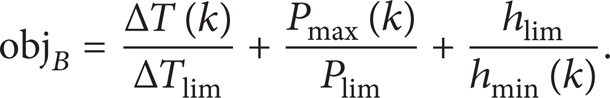
ob j_{B} = \frac{Δ T (k)}{Δ T_{\lim}} + \frac{P_{\max} (k)}{P_{\lim}} + \frac{h_{\lim}}{h_{\min} (k)} .

(20)

The first term controls the temperature rise. This performance is related to both the inlet temperature and the type of lubricant. The term indirectly controls the lubricant's dynamic viscosity and its degradation in time. In [22, 23], the continuous cycles of warming and cooling process degrade the lubricant making the temperature rise larger and the degradation process faster. The second term controls material properties and P_lim depends on the journal material choice. The third term controls the minimum film thickness. This performance has to be controlled to ensure that the bearing is working in a hydrodynamic regime and to indirectly introduce the manufacturing precision in the optimization process. In fact, h_min is calculated according to the roughness of the journal and shaft surface, which is controlled and typically has a value comprised between 0.2 and 1.6 μm both for the journal and the shaft. Usually the sleeve is a metal ring made of bronze or other materials and the shaft is made of steel. The common practice suggests keeping the minimum film thickness larger than the sum of Ra_J (the average roughness of the journal) and Ra_S (of the shaft). This avoids pure contact but does not avoid the possibility of EHD contacts [24, 25]. When the film thickness becomes comparable to the maximum roughness, the assumption of hydrodynamic lubrication regime (HDL) becomes not valid and performance predictions are not realistic. Furthermore, one has to consider the working precision, possible misalignments, and tolerances regarding the axial position of the groove. In the field of journal bearings, automotive industry and general mechanical industry want to prevent EHD regime which can be unreliable from the point of view of both journal degradation and lubricant degradation. Therefore, taking into account the possibility that the highest asperities can be softened or reduced by elastic work, another method is proposed; limit the film thickness to be greater than 3 μm between the highest asperities:

h_{\min} = 3 + (R a_{J} + R z_{J}^{+}) + (R a_{S} + R z_{S}^{+}) .

(21)

In this method, Rz_J⁺ is the average height of the 5 highest asperities in the profile measured from the nominal diameter line. The index J is used for the journal roughness and the S for the sleeve. 3 μm is the value chosen for this work but is nevertheless a variable value that can be adjusted depending on the manufacturing precision as well as the level of precision that all the calculation processes, in terms of input data, especially applied force, can reach.

The genetic search algorithm generates an input matrix for the objective function calculation. This matrix is X with dimensions [k, 3] where k is the number of subjects and 3 is the chosen number of decision variables. When the stochastic combination function generates a set of decision variables, it is also possible that it generates subjects where contact between journal and sleeve occurs (eccentricity ratio, ε, is equal or greater than 1). In previous literature, this problem was not addressed or taken care of by imposing custom eccentricity to contact subjects, oversight that affected their research [21]. Within this research, the algorithm calculates the contact subject's objective as follows:

{\begin{cases} ob j_{A} = 1.2, \\ ob j_{B} = (\max {ob j_{A}, ob j_{B}}) \cdot 1.2 . \end{cases}

(22)

Impeding the algorithm to generate these subjects can be detrimental to the whole search process. It is possible that in the search space near these subjects the algorithm will be able to find suitable solutions to improve the generation. Throughout this research, contact subjects were found but were rare. Furthermore, it was observed that through using the technique in (22), the contact subjects could not afford to pass to the next generation, but their “chromosomes” were used by the algorithm during the crossover process, which means that the GA was searching around them. Contact subjects can be found during the initialization of the algorithm when only the stochastic combinations are used to generate X . The use of 1.2 (which means adding a 20% to the maximum achievable score) is arbitrary. The practice suggests to do not give big penalizations to contact subjects. Usually the optimal solution and the contact subjects are found on the same variable space boundary but on opposite sides. Therefore, excluding the chromosomes of the contact subjects will lead to a longer calculation time, especially with GA.

It is interesting to note that this approach does not mathematically ensure the respect of the limits imposed for some performances, for example, temperature rise. In fact, while the objective ensures the minimization or maximization of the performances, it does not guarantee their complete control. For some problems, it is possible to have solutions in which performances exceed their limits and the designer must choose if their solution is still feasible. Only then is it possible to say that the limits can be considered fuzzy and their value can vary according to the problem. One example is the optimization of a bearing where the temperature rise limit is fixed to 10°C. If the optimized bearing reduces the power loss of 50% with respect to reference design and its temperature rise is 11°C, the idea of fuzzy limits suggests that the optimized bearing is feasible, even if the limits are not all satisfied.

The final optimization problem can be written as

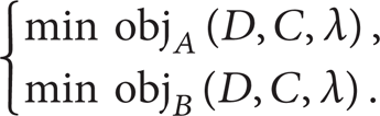
{\begin{cases} \min ob j_{A} (D, C, λ), \\ \min ob j_{B} (D, C, λ) . \end{cases}

(23)

The objective of the second stage is the nondimensional product between the maximum and the average temperature:

ob j_{T} = \frac{(T_{\max} (k) \cdot T_{ave} (k))}{\max {T_{\max} \cdot T_{ave}}} .

(24)

2.4. Genetic Algorithms

If the function is multivariable, the solution itself is multidimensional and the function is not regular, thus not derivable. Other tools have been developed to research the global minimum or maximum of the function. One of these tools was inspired by the theory of evolution and uses the rules of genetics to iterate the solution till convergence.

The main idea is to start with a set of random solutions where every solution has a set of chromosomes equal to the number of decision variables. The solution is evaluated in terms of fitness and the chromosomes are recombined using three tools that are derived from natural examples: crossover, mutation, and elite preservation. The continuous recombination of chromosomes produces solutions with increasing values of fitness since the highest score is found and the minimum or maximum of the objective functions is found.

A solution is defined as optimal or belonging to an optimal set if it lays on the Pareto Optimal Front, a group of nondominated solutions. In the case of minimization problems, the solution vector a dominates the solution vector b if and only if the following condition is fulfilled:

\begin{matrix} f_{i} (a) \leq f_{i} (b) \forall i = 1, \dots, m, \\ \exists j \in {1, \dots, m} : f_{i} (a) < f_{i} (b) . \end{matrix}

(25)

Above, f is the function to be minimized.

The parameters controlling the search for GA are number of generations, number of subjects, crossover factor, mutation factor, and elite count and the work flow is presented in Figure 6.

Figure 6:

In this scheme, the work flow of the genetic algorithm search is shown. PE is the performance function; “obj” is one of formulas (18) and (20). PA is the Pareto selection and GA is the modifier.

To ensure that the global minimum was found, the optimizations process has been repeated 2n + 1 (n number of decision variables) times. The first position is randomly generated and saved. In terms of the others, for every decision variable, a sufficient little Δx(i) is determined and the variations are sequentially added to the initial decision variable.

At the end of the optimization process, the solutions are usually nestled around the point of global minimum. Normally the diameter and the length to diameter ratio are converged while the clearance values are spread randomly in a range because the algorithm cannot further increase the precision (due to the discrete variable problem). The representative subject selected as the result of the optimization has the clearance to calculate as the average of the clearance values and is approximated to the nearest upper integer.

2.5. Artificial Bee Colony Algorithm

The artificial bee colony algorithm is an optimization method based on the intelligence behaviour of a honey bee swarm. ABC belongs to the category of particle swarm algorithms (PSO), which are methods inspired by the “collective intelligence” of populations, interactive agents, or swarms able to solve various problems following collective rules.

In particular, ABC algorithms imitate the behaviour of honey bees while foraging, demonstrating these smart insects’ ability to select the choicest of foods through basing their decision on several parameters like quality, quantity, taste, and the distance of the source. First, the bees randomly explore an area around the hive then communicate to the other bees the data regarding food sources in a “dancing area” (the communication hall of the hive). With successive repetitions and through exploring different areas, the bees are able to converge on the optimal food source, minimizing the distance and maximizing the quantity and quality of the nectar. From the standpoint of mechanical optimization, the food sources are the function value and the aim of the algorithm is to scout, following the explained logic, the objective space to find the optimal solution.

In the colony, the bees are divided in three types with each one playing a specific role: employees, onlookers, and scouts. The onlookers are those bees waiting in the dancing area for information about the food sources, the employees are those foraging the food and when a food source is exhausted the employee bee is forced to search a new one and, hence, becomes a scout bee.

In nature, the scouts are initially sent out to find new sources of food; they do so in a seemingly random order. However, once a new source is found, the scouts return to the hive and share their information with the onlookers in the dancing area, who then become employed and visit the new food source since that food source exists in their memory and has not been depleted yet. When the nectar is exhausted, the workers choose a new food source in the neighbourhood of the previous source based on the visual information that the bee has. At every flow, the workers’ dance is proportional to the nectar amount in the area just visited. The recruitment of onlookers is based on the intensity of the dance, so more bees are recruited from current workers that have visited sources with the highest nectar amount. Finally, an onlooker selects a new food source depending on the nectar information shared by all the workers generating a continuous modification of the optimal supply positions selected by bees.

In the ABC, the position of the food source represents the possible solution (the minimum of the function) and is a vector with the deciding variable values. The nectar amount represents the fitness (quality associated to the solution). The algorithm imitates the natural behaviour of bees except in the selection of new food sources. The comparison is made but the choice is not based on “visual information” (that is not available) but is randomly selected.

Every solution's position is a vector x (k) with k = (1, 2,…, l) with l number of food source and, consequently, the number of employed bees. After the initialization (random choice of food sources), the food sources are subjected to repeated cycles and the new positions are probabilistically chosen as follows:

prob (k) = \frac{fit (k)}{\sum_{k = 1}^{l} fit (k)} .

(26)

The algorithm used to produce a new food position from the old set of solutions is

v (k, i) = x (k, i) + υ (k, i) (x (k, i) - x (i i, i)) .

(27)

In this form, ii is the index for employed bees and is randomly chosen yet must be different to i. υ is a random factor (between [− 1 1]), controlling the selection of neighbourhood solutions. v(k, i) is the new candidate food source and using formula (27); all the optimization parameters are updated.

From the above explanation, it is clear that there are three control parameters that can influence the algorithm search. The first is l, or the number of food sources which are equal to the number of employed and onlooker bees (the proportion is fixed for the first release of Karaboga's algorithm but can be changed). The second parameter is the limit lim of times that a bee can visit the same food source. After that limit is reached, the source is abandoned. The last is the maximum number of cycles: mcn.

The ABC search gives the same results as the GA search but the evaluation of the functions are less numerous. Because this is already a demonstrated and well known fact [25], it is interesting to use ABC capabilities as search optimization solutions of different objective functions as they are built with the same logic as the one presented in Section 2.3. The following is a monoobjective function designed to further simplify the problem:

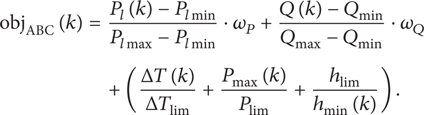
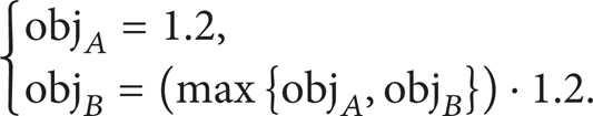
ob j_{ABC} (k) = \frac{P_{l} (k) - P_{l \min}}{P_{l \max} - P_{l \min}} \cdot ω_{P} + \frac{Q (k) - Q_{\min}}{Q_{\max} - Q_{\min}} \cdot ω_{Q} + (\frac{Δ T (k)}{Δ T_{\lim}} + \frac{P_{\max} (k)}{P_{\lim}} + \frac{h_{\lim}}{h_{\min} (k)}) .

(28)

The objective space is designed by the above function, and, in general, by any other possible function having different optimal solutions with respect to the objectives designed in Section 2.3. Nevertheless, if the design principles are the same, the different optimized solutions are feasible and a more realistic solution of the more general problem of HJB optimization. From the objectives, the fitness is calculated as

fit (k) = (M - obj (k)) .

(29)

The optimization is a minimum-minimum problem and the objectives are designed to have the optimal point corresponding to the universal minimum of the function. However, the fitness is the measure of the quality of the function and, in this case, the measure of the quality of the food source. Therefore, it is necessary to invert the function. For this problem, M is 1 for obj_A, is 3 for obj_B, and 4 for obj_ABC because the function has to express the relative percentage of quality with respect to the other solutions. ABC algorithm is not working in parallel and the fitness is calculated serially (like performance and objective) so a fixed parameter like M has to be used to generate the fitness. If the value of the objective is higher than M, only happening for obj_B and obj_ABC, the fitness was set to 0, 05. Also for ABC it is necessary to not lose solutions during the evaluation process so there is no loss of diversity. An advantage of the ABC algorithm is that it is easy to be implemented and a free version of the code (only for single objectives without fuzzy limits) can be found following the author's indications in [17].

2.6. Computational Fluid Dynamics

In the second stage of the work, the maximum temperature in the bearing is found with CFD analysis carried out with commercial tools: Ansys Fluent and Ansys Gambit, used in batch mode with Matlab. The CFD analysis is used because it is time efficient, has a good visualization of the results, does not require extensive programming skills, and has the ability to solve the full ThermoHydroDynamic (THD) field around the bearing. In [26] Moreno Nicolás et al., the author solved for the THD field around the bearing using the numerical network method. The present work has two aims: to solve the THD flow around the bearing and include the influence of the supply hole using this analysis. A good technique has been suggested by Brito et al. in [27], in which the system of PDE (Reynolds equation and energy equation) is solved with the use of a custom made FEM model. In this work, the capabilities of Ansys software are used to include the influence of the lubricant supply hole geometry on the maximum temperature of the bearing.

The geometrical model is made of a cylinder with diameter D subtracted from another cylinder with diameter D-2C. The external cylinder is translated and rotated in respect to the eccentricity and to the attitude angle. By creating the model in this way, the shaft is always centered and no further errors occur due to the geometrical tolerances that are introduced. Then, a cylinder with diameter d is attached to the external face of the lubricant domain. The axis of the cylinder passes through the centre of the bearing and lies on the x-y plane. The cylinder is then rotated on θ_s (positioning angle on the inlet).

There are two assumptions for the simulations: laminar flow and Reynolds cavitation model. The laminar flow assumption allows the avoidance of the use of turbulence models. The assumption is also verified in Figure 7 where the Reynolds number is shown (Reynolds number under 30 denotes full laminar regime).

Figure 7:

In this picture, the Reynolds number (ratio between inertial forces and viscous forces) is plotted for the journal surface.

The boundary conditions are the following.

Inlet: the inlet condition is “pressure inlet” with gauge total pressure 140 KPa and initial gauge pressure 0 Pa. The inlet temperature is set to T_in.

Outlet: the outlet condition is “pressure outlet” with static pressure set to 0 Pa. It should be pointed out that the operating pressure is set to 101325 Pa, so all the pressures at the boundaries are added to the operating pressure (absolute pressure = relative pressure + operating pressure). The initial condition of the outlet is applied to both side clearances of the journal bearing. The initial temperature of the outlet is set to the mixing temperature via UDF using formula (15).

Bearing: the boundary condition is “wall” with a static wall. The thermal model is “mixed,” the heat flux depends on the material, the free stream temperature is fixed at 320 K, the external emissivity is fixed to 1, the thickness is 2 mm, and the external radiation temperature is fixed to 300 K.

Shaft: the boundary condition is “wall” with rotating wall conditions. The speed is the rotational speed in rad/s and the centre of rotation is the axis of the shaft. The thermal model is “heat flux.” The value depends on the material but is decreased by 50% because the shaft does not have the opportunity to dissipate heat like the bearing housing.

The lubricant model is

μ = μ_{0} \cdot \exp (- β (T_{cell} - T_{in})) .

(30)

Here, μ₀ is the dynamic viscosity at ambient temperature and β is the thermo-viscosity-coefficient.

The simulations are controlled by Matlab, which commands Ansys Fluent and Ansys Gambit in batch mode. Two Matlab functions have been developed: the first generates the mesh file using Gambit, and the second solves the case and collect the data using Fluent. In both cases, Matlab writes a file, called a journal file, which is read by the two programs and contains the customized information about the geometry and solution process.

The lubricant film is divided in 20 layers in the radial direction and the discretization scheme is “cooper” with a mesh dimension 0.32 mm. The inlet channel has the same scheme and cell dimension of the lubricant in the clearance and the divisions along the channel are 75 with a length ratio of 0.95. The resulting number of cells is about 400000 with a solution time of 2 minutes for about 350 iterations, with residuals converging under the fixed tolerance of 10⁻⁶ (see Appendix C for details). For the simulations, three “user defined functions” (UDF) have been developed. The first iterates the viscosity value of every iteration following the model in (30). The second applies the Reynolds boundary conditions and iterates, if needed, the equilibrium position and the third collects the data and calculates the performance of the bearing.

3. Results and Discussion

The study case is a diesel internal combustion engine. At the design point, the point of maximum torque, the speed is 2500 rpm (246 rad/s), the torque is 326 Nm, the power is 85 kW, and the force acting on the bearing is 1750 N. The material of the shaft is steel; the material of the sleeve is bronze alloy; the inlet channel is a round hole in the upper bearing housing. The supply pressure is 140 KPa. The lubricant is 15W40 with μ₀ = 0.02 Pas and β = 0.038 1/K. The minimum diameter was calculated using Von-Mises criteria and the maximum was D_min, added to 30%. D_max is 34.2 mm and the minimum is 26.3 mm (Appendix A). The minimum length to diameter ratio is 0.3; the maximum is 0.9. The minimum clearance is C_min = 15 μm and the maximum is C_max = 30 μm. The force acted on the centre of the bearing; hence, L_f = 0. The limit choice has been done as follows.

Minimum film thickness: the choice is made with the use of formula (21). Values in the formula are all relative to the roughness of the bearing which is related to the diameter directly by mean of manufacturing relationships. The absolute value of 3 μm has been chosen according to work of Allmaier et al. [28] which prescribe 3 μm has the Elasto-Hydro-Dynamic (EHD) limit for car engine journal bearings.

Temperature rise: however, the choice of 20°C is a common choice the authors decided to further constrain the problem. Furthermore, 10°C limit is adopted by the two main references used for results comparison [12, 15]. The last reason why 10°C is chosen instead of 20°C is that a large amount of lubricants, without additives, suffer from rapid degradation due to temperature rise as explained in [2] specially if higher than 10°C.

Maximum pressure: the choice of 28 MPa has been made to impose a great constrain on pressure, because the future trend of hydrodynamic journal bearing is the use of polymeric materials in substitution of metal and the authors intentions are to demonstrate that is theoretically possible to accommodate this material choice.

The minimum supply diameter is 4 mm; the maximum is 9 mm. The inlet temperature is 25°C. The hole's position can be any suitable angular direction in the upper housing comprised between −65° and 65° (according to the scheme in Figure 2). The optimization parameters for the two techniques adopted are listed in Table 2.

Table 2:

Optimization parameters.

GA Parameters

Number of subjects	50
Maximum number of generations	50
Elite count	4
Crossover factor	0.65
Mutation	0.02
Calculation time	2–3 min

ABC parameters (stage I)

Number of food sources	100
Maximum number of cycles	20
Limit	100
Calculation time	<2 min

ABC for stage II

Number of food sources	28
Maximum number of cycles	10
Limit	10
Calculation time	14–15 min

The results of the optimization process are shown in Table 3. Here, the results obtained with different design techniques are listed. The design generated with Ghorbanian technique saves 39.8% power loss and over 50% of the mass flow. On the other hand, the combination of deciding variables generates a bearing with a minimum film thickness of 1.8 μm, a maximum pressure of 44 MPa, and a maximum temperature of 13.1°C. Despite the precision demonstrated in the calculations of the performances by the ANN in [12], the optimization objectives are too restrictive for a complete HJB analysis. The second technique is the one used by Hirani and Suh [15]. Here the dominance of the penalties on the objectives generates a bearing, which preserves temperature rise, maximum pressure, and film thickness while power loss and lubricant flow are penalized in the optimization.

Table 3:

Results of the optimization process.

	Weights		Decision variables			Performance							Control
	ω_P	ω_Q	D	C	λ	P _l		Q		ΔT	P _max	h _min	ω_cr	Q	ε
	[—]	[—]	[m]	[μm]	[—]	[W]	[%]	[m³/s]	[%]	[K]	[MPa]	[μm]	[rad/s]	[l/h]	[—]

Reference Design	—	—	0.0300	23	0.55	41.7		2.20E − 06		9.0	15.8	4.4	4627	7.90	0.81
Ghorbanian	—	—	0.0263	20	0.34	25.1	−39.84	1.02E − 06	−53.5	13.1	44.2	1.8	13984	3.68	0.91
Hirani	—	—	0.0300	24	0.88	53.0	26.99	3.15E − 06	43.5	6.7	8.7	7.6	2157	11.34	0.68
Optimal design (GA)	0.5	0.5	0.0263	20	0.72	35.3	−15.42	1.28E − 06	−41.7	8.7	14.7	4.5	3825	4.61	0.78
Optimal design (ABC)	0.5	0.5	0.0263	20	0.72	35.3	−15.42	1.28E − 06	−41.7	8.7	14.7	4.5	3825	4.61	0.78
Optimal design (obj_ABC)	0.5	0.5	0.0263	17	0.69	36.0	−13.74	1.45E − 06	−34.0	9.0	15.4	4.4	3346	5.22	0.74

The results of this work, concerning formula (18) and (20), are listed in the third and fourth row of Table 3. These two adopted techniques developed to find the minimum of the objective functions gave the same solution. The power loss is reduced by 15.4% and the mass flow is reduced by 41.7% with respect to the reference design. The temperature rise, maximum pressure, and the minimum film thickness are all under the imposed limits.

Concerning the results achieved using formula (28), they have the same tendency: reducing the mass flow and the power loss of 34% and 13.7%, respectively, and, at the same time, ensuring the respect of the limits. The advantage of this formulation is that it is monoobjective and the calculation time is 75% less in respect to the previous case with formula (18) and (20).

It is interesting to note, in Table 4, how the weights influence the optimization results. When ω_Q is 0.8, the power loss reduction is 1.6% and the search algorithm is modified for a strong mass flow reduction. When ω_P is 0.8, there is no reduction of the mass flow but the power consumption is reduced by 18.5%. 0.2 is the minimum value of the weights objective. This is because of the trade-off between the two performances chosen for objective in (18). The diameter is fixed to 26.30 mm, while the clearance tends to decrease while ω_Q increases and the length to diameter ratio is a bell shaped function.

Table 4:

Influence of the weights on the optimization results.

Weights		Decision variables			Performance							Control
ω_P	ω_Q	D	C	λ	P _l		Q		ΔT	P _max	h _min	ω_cr	S	ε
[—]	[—]	[m]	[μ m]	[—]	[W]	[%]	[m³/s]	[%]	[K]	[MPa]	[μm]	[rad/s]	[—]	[—]

0.8	0.2	0.0263	24	0.72	34.0	−18.5	2.29E − 06	4.3	7.7	18.0	4.6	4516	0.0569	0.81
0.7	0.3	0.0263	21	0.70	35.3	−15.4	1.68E − 06	−23.5	8.4	15.8	4.4	4183	0.0723	0.79
0.6	0.4	0.0263	19	0.70	34.3	−17.8	1.89E − 06	−13.8	9.4	15.4	4.3	3888	0.0883	0.77
0.5	0.5	0.0263	17	0.69	36.0	−13.7	1.45E − 06	−34.0	9.0	15.4	4.4	3346	0.1087	0.74
0.4	0.6	0.0263	16	0.74	38.0	−8.9	1.40E − 06	−36.4	9.4	13.9	4.9	2769	0.1317	0.70
0.3	0.7	0.0263	15	0.76	40.1	−3.9	1.30E − 06	−41.0	9.7	13.5	5.0	2580	0.1539	0.67
0.2	0.8	0.0263	15	0.78	41.1	−1.6	1.31E − 06	−40.2	10.7	13.1	5.2	2482	0.1579	0.65

Mathematically relating the weights to the applications or to the Sommerfield number is not possible because, for every different problem, different relationships are going to be found. Nevertheless, in order to help designers, it is possible to produce a table with generalized criteria, shown in Table 5.

Table 5:

Design criteria.

Weights		Criteria
ω_P	ω_Q
[—]	[—]

0.8	0.2	High speed and high precision bearings. ICE and turbochargers. Suitable also for those applications where the oil supply is not a key issue and the supply system is oversized.
0.7	0.3

0.6	0.4	This range of solutions is good for every application and does not unbalance the search in a critical way. In this field have to work all those designers who are not sure about thermal and dynamic behaviour of the bearing.
0.5	0.5
0.4	0.6

0.3	0.7	Low speed and high load. This choice is not suitable in the case where the temperature is a key issue for the bearing.
0.2	0.8

Dynamic viscosity has a great effect on the bearing performance and on the optimization process as shown in Table 6. When the viscosity decreases, power loss and mass flow decrease. The temperature rise is also increased with the viscosity. Both Tables 3 and 4 constitute maps for designers. The choice of dynamic viscosity is related to the project and the choice of the weights is related to the working conditions of the bearing.

Table 6:

Influence of dynamic viscosity on the optimization results.

Viscosity	Decision variables			Performance					Control
Viscosity	D	C	λ	Pl	Q	ΔT	P _max	h _min	ω_cr	S	ε
[Pas]	[m]	[µm]	[—]	[W]	[m³/s]	[K]	[MPa]	[µm]	[rad/s]	[—]	[—]

ω_P = 0.8 and ω_Q = 0.2
0.005	0.0263	15	0.89	17.8	1.69E − 06	5.1	11.4	3.5	4171	0.0450	0.77
0.01	0.0263	16	0.90	22.6	1.79E − 06	5.8	11.4	3.4	4685	0.0800	0.79
0.015	0.0263	21	0.82	24.2	2.22E − 06	5.4	13.8	3.2	6916	0.0635	0.85
0.02	0.0263	24	0.72	34.0	2.29E − 06	7.0	14.4	4.4	4849	0.0569	0.82
0.03	0.0263	29	0.64	39.0	2.50E − 06	7.7	18.0	4.6	5537	0.0520	0.84
0.04	0.0263	30	0.55	43.4	2.75E − 06	9.5	21.3	4.6	5732	0.0556	0.85

ω_P = 0.2 and ω_Q = 0.8
0.005	0.0266	15	0.89	18.3	1.73E − 06	5.2	11.5	2.9	5633	0.0471	0.81
0.01	0.0263	15	0.83	27.0	1.53E − 06	7.6	12.2	3.8	3677	0.0840	0.75
0.015	0.0263	15	0.80	34.2	1.40E − 06	9.8	12.8	4.6	2833	0.1215	0.69
0.02	0.0263	15	0.78	41.8	1.32E − 06	10.2	13.2	5.2	2505	0.1579	0.66
0.03	0.0263	16	0.76	53.0	1.30E − 06	14.0	13.7	6.0	2247	0.2029	0.63
0.04	0.0263	18	0.71	59.6	1.24E − 06	15.0	14.5	6.7	2130	0.1996	0.63

ω_P = 0.5 and ω_Q = 0.5
0.005	0.0264	15	0.89	18.5	1.70E − 06	5.1	11.6	3.0	5334	0.0457	0.80
0.01	0.0263	15	0.84	26.5	1.53E − 06	7.5	11.2	3.8	3677	0.0850	0.75
0.015	0.0263	15	0.77	33.2	1.37E − 06	10.0	13.0	4.4	2995	0.1169	0.71
0.02	0.0263	17	0.72	37.3	1.48E − 06	10.6	14.5	4.7	3045	0.1135	0.72
0.03	0.0263	20	0.63	43.2	1.58E − 06	12.0	16.9	5.0	3249	0.1076	0.75
0.04	0.0263	24	0.57	46.8	1.79E − 06	12.2	19.6	5.1	3825	0.0901	0.79

And so the optimal set is selected: D = 26.30 mm, C = 17 μm, and λ = 0.69 (L = 18.15 mm). For this configuration, the optimization of the inlet channel position and dimension was carried out using ABC, CFD, and obj_T. The ABC algorithm is used to minimize the nondimensional product between T_max and T_ave, which is plotted in Figure 8(c). From this figure, in simple cases, it is possible to note that the minimum point is 0.9430, which corresponds to the decision variable coordinates: θ_s = 15° and d_in = 9 mm (which are also the values found within the ABC research).

Figure 8:

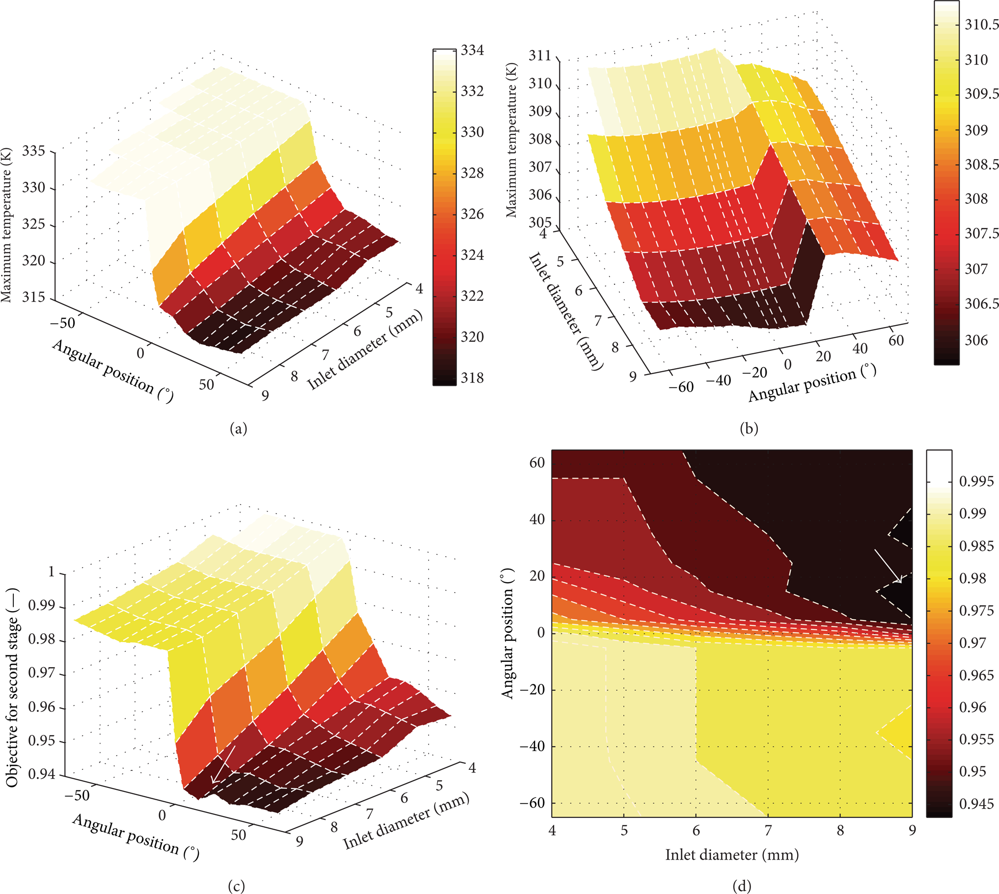
(a) Graph showing the maximum temperature distribution. (b) Graph showing the average temperature in the bearing. (c) Graph showing the objective space for the second stage of the optimization. (d) Contours of objective value (formula (24)). The white arrow shows the minimum point.

In Figure 8(a), the maximum temperature is shown. More of the inlet channel is nearer to the “warm zone” (the minimum thickness zone in the convergent-divergent channel) while more of the maximum temperature has decreased. On the other hand, the average temperature increases because the capability of the inlet channel walls is progressively decreasing. In fact, the average temperature, Figure 8(b), increases when the inclination of the channel is higher than 20° and when the channel is near the warm zone. While θ_s is increasing, the average temperature has a minor decrease, due to the inflow from the outlet, of fresh fluid, which is set to the mixing temperature via UDF (Figure 9).

Figure 9:

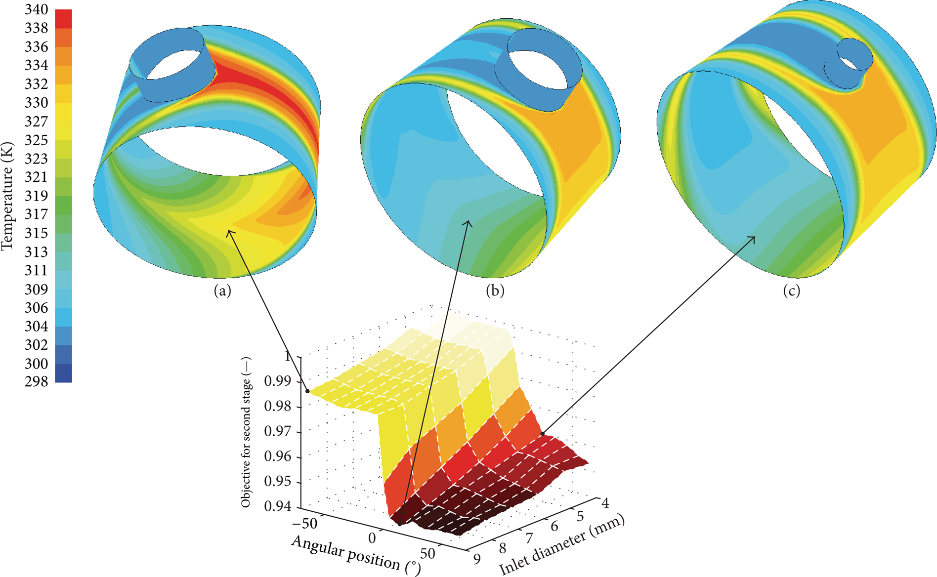
The figure is showing the temperature field in the bearings in different angular positions with different inlet diameters.

The fact that the optimal diameter rests on the edge of the research space means that the multidimensional objective function has its global minimum on the boundary of this same space. If the research space could be increased, another global minimum would be found. This fact confirms the theory on which this optimization process is designed: only an objective able to take into account several decision variables and fuzzy limits would be able to solve the problem of HJB optimization. Ideally, if the diameter could be set to zero, no friction and mass flow would be present, and the objectives would be minimized to an unrealistic value for D. From this point onward, there is a need to calculate the research space boundaries.

4. Conclusions

An ANN is used to fast and accurately predict the performances of HJB. Due to its nature, the ANN tool is flexible and can be adapted to any kind of bearing and working behaviour if a suitable set of examples are used for training. The strategy proposed is to divide the network into a number of smaller networks working in parallel to improve the single network capabilities and without the inflation of the network.

The problem is divided into two stages to magnify the influence of the single set of deciding variables. For every stage, different performance functions, decision variables, and objectives were designed.

In order to take into account the viscosity as a decision variable in the design, a realistic optimization work-flow was designed and optimization maps were built.

The present work demonstrates how it is possible to reduce power loss and mass flow while controlling the temperature rise and the maximum temperature by optimizing the choice of journal bearing design parameters. At the same time, the mathematical optimization of the objectives gives realistic results, and, in terms of manufacturability, they give the designer the opportunity to choose how to modulate the design process and dynamic viscosity.

Footnotes

Appendices

Nomenclature

Conflict of Interests

The authors declare that there is no conflict of interests regarding the publication of this paper.

Acknowledgment

The work was supported by Grant from The working Behaviour and the Lubricant Mechanism of High-Quality Synthetic Lubricants in Aero-power Transmission Systems (2013CB632305).

References

Holmberg

Andersson

, and Erdemir

, “Global energy consumption due to friction in passenger cars,” Tribology International, vol. 47, pp. 221–234, 2012.

Zengeya

and Gadala

, “Empirically derived optimization model: theoretical formulation and validation,” Tribology International, vol. 47, pp. 145–158, 2012.

Hirani

Rao

T. V. V. L. N.

Athre

, and Biswas

, “Rapid performance evaluation of journal bearings,” Tribology International, vol. 30, no. 11, pp. 825–832, 1997.

Vignolo

G. G.

Barilá

D. O.

, and Quinzani

L. M.

, “Approximate analytical solution to Reynolds equation for finite length journal bearings,” Tribology International, vol. 44, no. 10, pp. 1089–1099, 2011.

Sun

and Changlin

, “Hydrodynamic lubrication analysis of journal bearing considering misalignment caused by shaft deformation,” Tribology International, vol. 37, no. 10, pp. 841–848, 2004.

Naduvinamani

N. B.

and Patil

S. B.

, “Numerical solution of finite modified Reynolds equation for couple stress squeeze film lubrication of porous journal bearings,” Computers and Structures, vol. 87, no. 21–22, pp. 1287–1295, 2009.

Carbonara

A. F.

Duarte

Jr. , and Bittencourt

M. L.

, “Comparison of journal orbits under hydrodynamic lubrication regime for traditional and Newton-Euler loads in combustion engines,” Latin American Journal of Solids and Structures, vol. 6, no. 1, pp. 13–33, 2009.

Jang

J. Y.

and Khonsari

M. M.

, “Design of bearings on the basis of thermohydrodynamic analysis,” Proceedings of the Institution of Mechanical Engineers J: Journal of Engineering Tribology, vol. 218, no. 5, pp. 355–363, 2004.

Hirani

and Biswas

, “A hybrid solution scheme for performance evaluation of crankshaft bearings,” Journal of Tribology, vol. 122, no. 4, pp. 733–740, 2000.

10.

Chasalevris

and Sfyris

, “Evaluation of the finite journal bearing characteristics, using the exact analytical solution of the Reynolds equation,” Tribology International, vol. 57, pp. 216–234, 2013.

11.

Zengeya

and Gadala

, “Optimization of journal bearings usigng a hybrid scheme,” Proceedings of the Institution of Mechanical Engineers J: Journal of Engineering Tribology, vol. 221, no. 5, pp. 591–607, 2007.

12.

Ghorbanian

Ahmadi

, and Soltani

, “Design predictive tool and optimization of journal bearing using neural network model and multi-objective genetic algorithm,” Scientia Iranica, vol. 18, no. 5, pp. 1095–1105, 2011.

13.

Gertzos

K. P.

Nikolakopoulos

P. G.

, and Papadopoulos

C. A.

, “CFD analysis of journal bearing hydrodynamic lubrication by Bingham lubricant,” Tribology International, vol. 41, no. 12, pp. 1190–1204, 2008.

14.

Bompos

D. A.

and Nikolakopoulos

P. G.

, “CFD simulation of magnetorheological fluid journal bearings,” Simulation Modelling Practice and Theory, vol. 19, no. 4, pp. 1035–1060, 2011.

15.

Hirani

and Suh

N. P.

, “Journal bearing design using multi-objective genetic algorithm and axiomatic design approaches,” Tribology International, vol. 38, no. 5, pp. 481–491, 2005.

16.

Boedo

and Eshkabilov

S. L.

, “Optimal shape design of steadily loaded journal bearings using genetic algorithms,” Tribology Transactions, vol. 46, no. 1, pp. 134–143, 2003.

17.

Karaboga

and Akay

, “A comparative study of Artificial Bee Colony algorithm,” Applied Mathematics and Computation, vol. 214, no. 1, pp. 108–132, 2009.

18.

Sonmez

, “Multi-objective environmental/economic dispatch solution with penalty factor using artificial bee colony algorithm,” Scientific Research and Essays, vol. 6, no. 13, pp. 2824–2831, 2011.

19.

Anandhakumar

Subramanian

, and Ganesan

, “Modified ABC algorithm for generator maintenance scheduling,” International Journal of Computer and Electrical Engineering, vol. 3, pp. 1–8, 2011.

20.

Singhal

and Khonsari

M. M.

, “A simplified thermohydrodynamic stability analysis of journal bearings,” Proceedings of the Institution of Mechanical Engineers J: Journal of Engineering Tribology, vol. 219, no. 3, pp. 225–234, 2005.

21.

Howlet

R. J.

Zoysa

M. M.

Walters

S. D.

, and Howson

P. A.

, “Neural network techniques for monitoring and control of internal combustion engines,” in Proceedings of the International Symposium on Intelligent Industrial Automation, 1999.

22.

Mascolo

Rausa

Bagnuolo

Mininni

, and Tinucci

, “Thermal degradation of synthetic lubricants under oxidative pyrolytic conditions,” Journal of Analytical and Applied Pyrolysis, vol. 75, no. 2, pp. 167–173, 2006.

23.

Toujou

Tsukamoto

, and Matsuoka

, “Characterization of lubricants for fluid dynamic bearing by TOF-SIMS,” Applied Surface Science, vol. 203–204, pp. 590–595, 2003.

24.

Chu

H.-M.

W.-L.

, and Chang

Y.-P.

, “Thin film elastohydrodynamic lubrication-a power-law fluid model,” Tribology International, vol. 39, no. 11, pp. 1474–1481, 2006.

25.

Seabra

Sottomayor

, and Campos

, “Non-Newtonian EHL model for traction evaluation in a roller-inner ring contact in a roller bearing,” Wear, vol. 195, no. 1–2, pp. 53–65, 1996.

26.

Nicolás

J. A. Moreno

de León Hijes

F. C. Gómez

, and Alhama

, “Solution of temperature fields in hydrodynamics bearings by the numerical network method,” Tribology International, vol. 40, no. 1, pp. 139–145, 2007.

27.

Brito

F. P.

Miranda

A. S.

Claro

J. C. P.

, and Fillon

, “Experimental comparison of the performance of journal bearing with a single and twin axial groove configuration,” Tribology International, vol. 54, pp. 1–8, 2012.

28.

Allmaier

Priestner

Six

Priebsch

H. H.

Forstner

, and Novotny-Farkas

, “Predicting friction reliably and accurately in journal bearings—a systematic validation of simulation results with experimental measurements,” Tribology International, vol. 44, no. 10, pp. 1151–1160, 2011.

29.

http://www.lucefin.com/wp-content/files_mf/42crmo4astmen.pdf.

30.

http://www.mathworks.fr/fr/help/symbolic/solve.html.

31.

Costa

Fillon

Miranda

A. S.

, and Claro

J. C. P.

, “An experimental investigation of the effect of groove location and supply pressure on the THD performance of a steadily loaded journal bearing,” ASME Journal of Tribology, no. 122, pp. 227–232, 2000.

32.

Ansys Fluent Theory Guide, April 2009.

Journal Bearing Optimization Using Nonsorted Genetic Algorithm and Artificial Bee Colony Algorithm

Abstract

1. Introduction

2. Optimization Methodology

2.1. Optimization Strategy

2.2. Performance Calculation

2.3. Objective Definition

2.4. Genetic Algorithms

2.5. Artificial Bee Colony Algorithm

2.6. Computational Fluid Dynamics

3. Results and Discussion

4. Conclusions

Footnotes

Appendices

Nomenclature

Conflict of Interests

Acknowledgment

References