
Abstract
Matrix theory plays an important role in modeling linear systems in engineering and science. To model and analyze the intricate behavior of complex systems, it is imperative to formalize matrix theory in a metalogic setting. This paper presents the higher-order logic (HOL) formalization of the vector space and matrix theory in the HOL4 theorem proving system. Formalized theories include formal definitions of real vectors and matrices, algebraic properties, and determinants, which are verified in HOL4. Two case studies, modeling and verifying composite two-port networks and state transfer equations, are presented to demonstrate the applicability and effectiveness of our work.
1. Introduction
The matrix theory is a core subbranch of linear algebra. Matrices as operators of linear space transformations play important roles in modeling linear systems. The matrix theory has extended applications in most of science fields. In many branches of physics, including classical mechanics, optics, electromagnetism, quantum mechanics, and quantum electrodynamics, the matrix theory is used to analyze physical phenomena, such as the motion of rigid bodies. In computer graphics, matrices are used to perform 2-dimensional and 3-dimensional projection transformation. In robotics, matrices are used to address robot kinematics and dynamics. In probability theory and statistics, stochastic matrices are used to describe sets of probabilities; for instance, matrix decomposition supports modeling information compression, reconstruction, and retrieval. Matrix calculus generalizes classical analytical notions such as derivatives and exponentials to higher dimensions. Furthermore, the modern matrix theory covers subjects related to many other important mathematical branches such as graphs, combinatorics, and statistics. MATLAB's success is the typical sample of matrix applications.
Traditionally, a number of efficient numerical analysis algorithms were developed for matrix computations in order to improve the accuracy of results, yet the absolute precision in the real number field can never be reached because of round-off error, approximate algorithms to address large-scale issues, and so on. On the other hand, the property analysis of linear system based models has been done using paper-and-pencil proof methods, which is quite error prone. A tiny error or inaccuracy, however, may result in failure or even loss of lives in highly sensitive and safety-critical engineering applications. Mechanical theorem proving, on the contrary, is capable of performing precise and scalable analysis.
Mechanical theorem proving has been considered a promising and powerful method of formal proofs in pure mathematics or system analysis and verification [1–5]. Systems or any proof goals need to be modeled formally before they are verified by theorem provers, and theorem provers work based on logic theorem libraries of mathematics. The more mathematic theorem libraries there are, the wider the scope of application of the theorem provers is [5]. It is significant to formalize matrix theory in theorem provers for extending theorem proving applications. The parts of the matrix theories have been formalized in some theorem provers. Nakamura et al. [6] presented the formalization of the matrix theory in Mizar in 2006. The COQ system has also started to provide matrices in recent years [7]. Harrison presented the formalization of Euclidean space in the HOL-light system in 2005 [8]. In Isabelle/HOL [9], some basic matrix theory has been formalized in [10, 11]. However, the HOL4 [12], which is the latest version of the HOL theorem prover, does not yet have a matrix theory in its formalized theories collections. Furthermore, no successful conversion of matrix theory from any other theorem prover can be found in the current literature. For this reason, diverse applications are not available to be verified using HOL4. For example, Liu et al. [13] presented a sophisticated formalization in HOL4 for the finite-state discrete-time Markov Chain theory which is widely used to model random processes in physical and informational systems. Without the formalized matrix theory, the state transition matrix was formalized by the list type instead of the matrix type. If our matrix theory were used to supply the formalization of Markov chain, the work in [13] would be enhanced to efficiently address scalable systems. Hence, formalizing the matrix theory in HOL4 enables formally analyzing linear system models using this theorem prover, as well as benefiting the development of enormous other theories, such as Markov chain.
We will formalize the matrix analysis theories by stages. This paper presents a systematic formalization of the matrix algebraic theory in the HOL4 system. It includes the formalization of vectors and matrices and proofs of their relevant algebraic properties. The vector and matrix are defined based on the finite Cartesian products (FCP) library of HOL4. The properties of vectors, matrices, and determinants are characterized in accordance with linear space properties. As case studies of applications, the formal modeling and proof of the parameterized two-port networks and high-speed power of matrix solution to state transfer equations are presented. In this paper, we use HOL4 notations, and some notations are listed in Table 1.
Some HOL4 notations and their semantics.

This paper is organized as follows. Section 2 proposes the formalization of the vector space. Then, the formalization of the fundamental matrix theory is presented in Section 3. Two applications of modeling and verifying by the proposed approach are presented in Section 4. Section 5 concludes the paper.
2. Formalization of Vector Space
Matrices are transforming operators in the vector space. In this section, vectors and their algebraic operations are formalized based on the FCP library in HOL4, and the linear properties of vector space are proven.
2.1. Defining the Data Type of Vectors
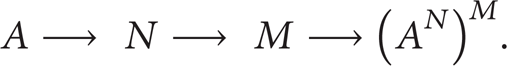
N-dimensional vectors are elements of an N-dimensional vector space, denoted by A N , where A is the element type and N is a number variable for the dimension. A N can be constructed by the N-dimensional Cartesian products of A. The function space is as follows:

It is not trivial to define the compound type in the HOL4 system based on a simple type theory where a compound type can only depend on other types and not on terms. Harrison [8] introduced an elegant method of defining the vector type in the HOL-light theorem prover. We define n-dimensional vectors in HOL4 following Harrison's method, with the cardinality of the type being the dimension of the Cartesian product. The FCP theory was implemented and named the fcpTheory in HOL4. Assuming A to be a real type and n the index type, the real vector type is constructed based on the fcpTheory in HOL4 as follows:

where 'n stands for a type variable, which can be instantiated by a certain type. The elements of a vector are operated using the indexing operator “‘” (or, alternatively, %%) in the fcpTheory. For example, the ith element of a vector, which is written as x i in mathematics, is denoted by “x' i” (or x %% i). According to the fcpTheory, two vectors are equal if and only if their corresponding elements are equal.
2.2. Formalizing the Operations of Vectors
This subsection gives the formalization of the operations of N-dimensional vectors. The arithmetic operations of vectors are pointwise on elements of the vectors. In order to conveniently deal with the issue of dimensionality and eliminate the problem of interaction with the FCP binder, two mapping functions are given to simplify the operating of all of the elements of vectors and matrices:
Definition 1 (vec_map_def). Consider the following:
|- !f v. vector_map f v = FCP i. f (v ' i).
Definition 2 (vec_map2_def). Consider the following:
|- !f v1 v2. vector_map2 f v1 v2 = FCP i. f (v1 ' i) (v2 ' i)
where the symbol “|-” is the preceding turnstile for definitions and theorems and “FCP i” means for all 0<= i < size of vectors. Obviously, here “FCP i” has better readability and more expressive power than the lambda calculus “∖i,” which does not bound “i” implicitly. The above two definitions are for one and two vectors, respectively. The definitions of addition, subtraction, and negative operators on vectors are given based on the two mapping functions. For readability, “+” and “−” are overloaded to denote addition and subtraction; “∼” denotes negative; and the dollar symbol in front of an operator indicates that the operator has a special syntactic status.
Definition 3 (vector_add_def). Consider the following:
|- $ + = vector_map2 $ +.
Definition 4 (vector_sub_def). Consider the following:
|- $− = vector_map2 $−.
Definition 5 (vector_neg_def). Consider the following:
|- $∼ = vector_map numeric_negate.
Two kinds of products of vectors are implemented. One is the inner product of vectors:

The symbol “∑” can be presented by the following function in realTheory:
|- !f n m. (sum (n, 0) f = 0) ∧ (sum (n, SUC m) f = sum (n, m) f + f (n + m)).
We overload “**” for the multiplication of vectors. The inner product (dot product) of two vectors is defined as follows.
Definition 6 (vector_dot_def). Consider the following:
|- !x y. x ** y = sum (0, dimindex (:'n)) (∖i. x ' i * y ' i).
Note that n is a type variable; thus, dimindex is used to obtain the cardinality of the type. Another is a scalar product operation, which multiplies a vector by a scalar. This includes two cases: the scalar may be at the right or left side.
Definition 7 (vector_rmul_def). Consider the following:
|- !k v. k ** v = FCP i. k * v ' i.
Definition 8 (vector_lmul_def). Consider the following:
|- !v k. v ** k = FCP i. v ' i * k.
We present two special vectors: the zero vector and the base vectors.
Definition 9 (vector_0_def). Consider the following:
|- vector_0 = FCP i. 0.
Definition 10 (vector_basis_def). Consider the following:
|- !k. vector_basis k = FCP i. if i = k then 1 else 0.
2.3. Proofs of the Algebraic Properties of Vectors
In this subsection, the algebraic properties of vectors are formalized and verified. Most of the properties are linear properties, because vector space is linear space. Table 2 shows the formalization of these properties.
The formalization of the algebraic properties of vectors.
In Table 2,

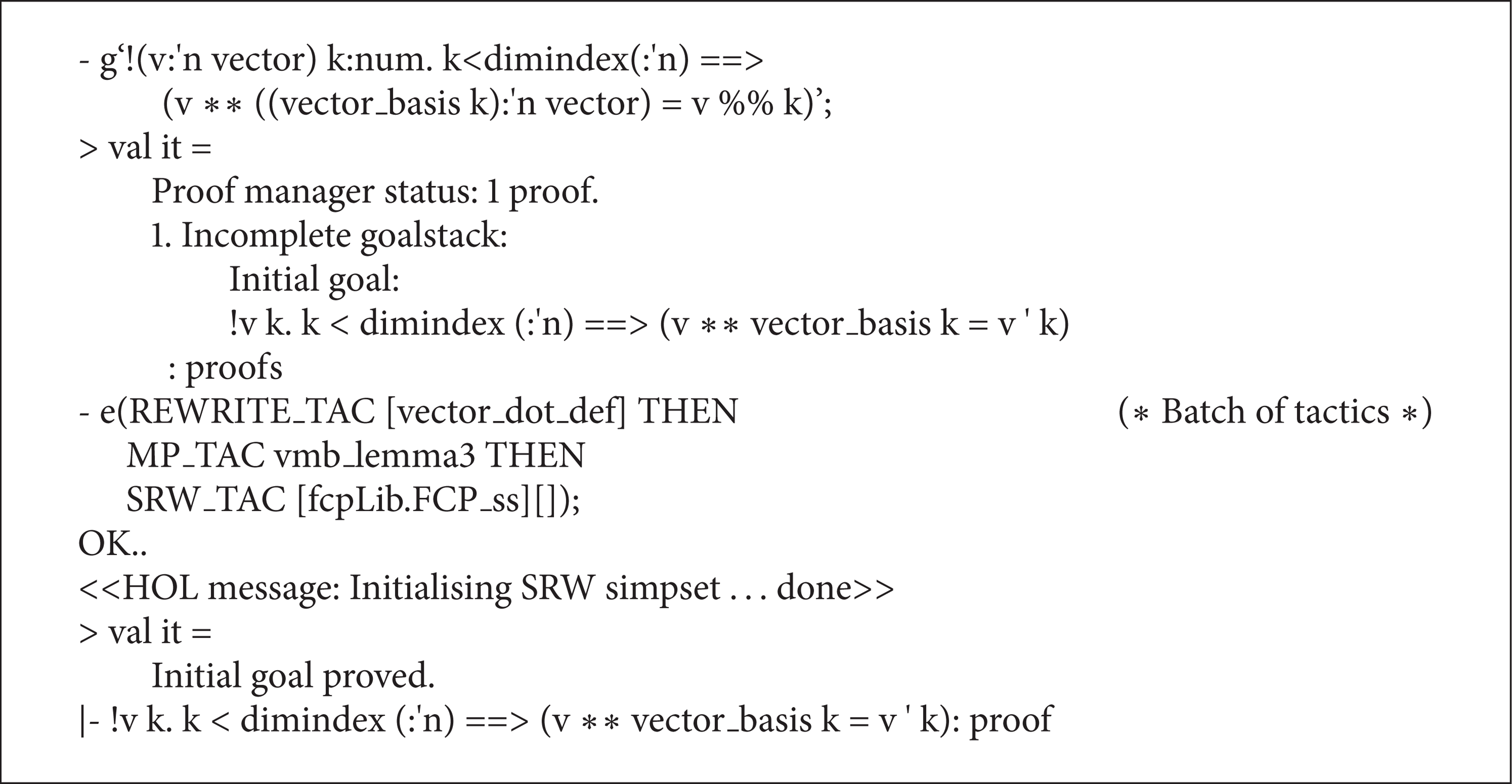
The interactive proof of the property VECTOR_MUL_BASIS.
Lemma 1 (vmb_lemma1). Consider the following:
|- !v k. k < dimindex (:'n) ==>
(sum (0, dimindex (:'n)) (∖i. v ' i * vector_basis k ' i) =
sum (0, dimindex (:'n)) (∖i. if i = k then v ' k else 0)).
Lemma 2 (vmb_lemma2). Consider the following:
|- !v k. k < dimindex (:'n) ==>
(sum (0, dimindex (:'n)) (∖i. if i = k then v ' k else 0) = v ' k).
Based on Lemmas 1 and 2, it is easy to prove Lemma 3.
Lemma 3 (vmb_lemma3). Consider the following:
|- !v k.
k < dimindex (:'n) ==>
(sum (0, dimindex (:'n)) (∖i. v ' i * vector_basis k ' i) = v ' k).
Algorithm 1 shows the detailed interaction of proving the property VECTOR_MUL_BASIS, where “-” is the command prompt in HOL4; “g” guides the proving goal; “e” guides the tactics of proving; “>” is the echo prompt; and “|-” guides the goal or subgoal that is proved. If all of the tactics involved in the proof are known, they can be sequenced together with “THEN” to construct a batch-command style process. The batch-command style proving process takes just one step, as shown in Algorithm 2.
The batch-command proof of the property VECTOR_MUL_BASIS.
Choosing strategies and theorems for each step of proofs is tedious work. Fortunately, to some extent decision procedures can help to automatically produce a proof. In practice, a simple decision procedure named VECTOR_ARITH_TAC is developed by putting together many potentially useful theorems, definitions, and strategies. The decision procedure is shown in Algorithm 3. This procedure can automatically prove most of the arithmetic properties of vectors.

The decision procedure for vector arithmetic.
3. Formalization of Fundamental Matrix Theory
3.1. Defining the Data Type of Matrices
A matrix is a two-dimensional array of numbers with many rows and columns. A matrix type is defined in the same way as a vector type. A row or a column of a matrix is a vector; thus, we use a Cartesian product twice to present the M × N matrix type:
The HOL4 type is written as follows:

As with vectors, one can generally use “x ' i ' j” where informally one would write x ij for indexing. The fcpTheory can ensure that two matrices are equal if and only if their corresponding elements are equal.
3.2. Formalizing the Operations of Matrices
This subsection presents the formalization of the arithmetic operations of matrix theory. The arithmetic operations of matrices are pointwise on elements of matrices. The mapping function for vectors can be easily generalized to matrix type, given as follows.
Definition 11 (matrix_map_def). Consider the following:
|- !f m. matrix_map f m = FCP i j. f (m ' i ' j).
Definition 12 (matrix_map2_def). Consider the following:
|- !f m1 m2. matrix_map2 f m1 m2 = FCP i j. f (m1 ' i ' j) (m2 ' i ' j).
The usual operations of addition, subtraction, and negation of matrices are defined as follows.
Definition 13 (matrix_add_def). Consider the following:
|- matrix_add = matrix_map2 $ +.
Definition 14 (matrix_sub_def). Consider the following:
|- matrix_sub = matrix_map2 $−.
Definition 15 (matrix_neg_def). Consider the following:
|- matrix_neg = matrix_map numeric_negate.
These operations are defined based on the mapping functions. Obviously, the matrices involved in addition and subtraction must have the same number of rows and columns, and the elements of both matrices are dealt with in the same order.
The multiplication of matrices is based on the inner products of vectors. Therefore, this operation is defined after the definitions of the row extracting and the column extracting operations. Letting A, B be matrices of R, the definitions are as follows.
Definition 16 (row_def). Consider the following:
|- !A k. row A k = FCP j. A ' k ' j.
Definition 17 (column_def). Consider the following:
|- !A k. column A k = FCP i. A ' i ' k.
Definition 18 (matrix_prod_def). Consider the following:
!A B. A ** B = FCP i j. row A i ** column B j.
Note that the dimension of the rows of matrix A must be equal to the number of columns of matrix B. This requirement must be satisfied to obtain the inner product of vectors.
In addition, other operations are defined, such as transposition, multiplication with a vector or a real number, and exponentiation.
Definition 19 (matrix_transp_def). Consider the following:
|- !A. transp A = FCP i j. A ' j ' i.
Definition 20 (matrix_lmul_vector_def). Consider the following:
|- !v A. v ** A = FCP i. v ** column A i.
Definition 21 (matrix_rmul_vector_def). Consider the following:
|- !A v. A ** v = FCP i. row A i ** v.
Definition 22 (matrix_lmul_scalar_def). Consider the following:
|- !k A. k ** A = FCP i j. k * A ' i ' j.
Definition 23 (matrix_rmul_scalar_def). Consider the following:
|- !A k. A ** k = FCP i j. A ' i ' j * k.
Definition 24 (matrix_pow_def). Consider the following:
|- (!A. matrix_pow A 0 = matrix_E) ∧ !A k. matrix_pow A (SUC k) = A ** matrix_pow A k.
Inverse matrices are useful for many applications, such as analyzing groups of linear equations. We present the definition, which says that a square matrix may have an inverse matrix, after the definition of the identity matrix.
Definition 25 (matrix_E_def). Consider the following:
|- matrix_E = FCP i j. if i = j then 1 else 0.
Definition 26 (matrix_inv_def). Consider the following:
|- !A. matrix_inv A <=> ?A'. (A ** A' = matrix_E) ∧ (A' ** A = matrix_E).
The definition of the zero matrix, whose elements are all 0, is given as follow.
Definition 27 (matrix_0_def). Consider the following:
|- matrix_0 = FCP i j. 0.
3.3. Verification of the Algebraic Properties of Matrices
The fundamental algebraic properties of matrices are formalized and verified in this subsection. The properties are formally modeled in terms of the above definitions and shown in Table 3.
The formalization of the fundamental algebraic properties of the matrix operation.
The properties are proven in a pointwise way based on the definitions of the matrix operations and the vector properties. As an example, we present proofs of a frequently used property named MATRIX_MUL_ASSOC. To reduce proofs of the properties, the lemmas in Table 4 are proved in advance.
The lemmas for proving MATRIX_MUL_ASSOC.

Algorithm 4 shows the proof of MATRIX_MUL_ASSOC. First, the definitions of matrix_prod_def, row_FCP, and column_FCP are used to expand matrix products into vector products, and then the definition of vector_dot_def is used to expand the vector products into summations of real products. Finally, the conclusion that the corresponding elements of both sides are equal is drawn. Only the batch-command style proving process is shown in Algorithm 4.

The compact process of proving the property MATRIX_MUL_ASSOC.
The formalization of these theorems forms a base of reasoning for the transformation of the linear system.
Some special matrices play important parts in applications. For example, the square matrix applies on the determinant. In the next subsection, we will present the formalization of determinant.
3.4. Formalization of the Determinant
In the matrix theory, the determinant is a value defined only for square matrices and indicates discriminative information. When the matrix is that of the coefficients of a group of linear equations, that the determinant is nonzero or zero determines that the system has a unique solution exactly or there are either no solutions or many solutions, respectively. When the matrix corresponds to a linear transformation of a vector space, the nonzero determinant means that the transformation has an inverse operation. In this subsection, we present the formalization of the determinant.
The determinant of a square matrix A is evaluated by the entries of A. The determinant of a matrix of arbitrary size can be defined by the Leibniz formula:
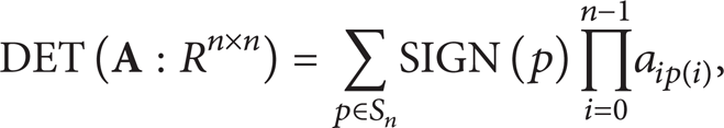
where aip(i) is the entry of ith row and p(i) column of
Definition 28 (determinant). Consider the following:
|- DET(A:('n, 'n) matrix) =
SUM {p ∣ pPERMUTEScount(dimindex(:'n))}
(∖p. SIGN(p) * (PRODUCT (count(dimindex (:'n))) (∖i. A ' i ' (p i)))),
where permutation is defined by
|- p PERMUTES s = (!x. x NOT IN s ==> p x = x) ∧ (!y. ?!x. p x = y).
The definition claims that p is a permutation of a set of natural numbers s. Informally, a permutation of a set of natural numbers is an arrangement of those natural numbers into a particular order. In the above formal definition, for any natural number y, there must exist a position x of permutation p where y dwells. It is a sophisticated definition rather than a trivial translation.
The signature of a permutation p is denoted by SIGN p and defined as + 1 if p is even and −1 if p is odd.
Consider the following:
|-(SIGN p):real = if EVENPERM p then &1 else − &1.
The function EVENPERM estimates the parity of a permutation. The parity of a permutation p can be estimated by the parity of the times of swap operating for transforming the identity permutation, denoted by I, into p. EVENPERM is defined as follows:
|- EVENPERM p = EVEN(@n. SWAPSEQ n p),
where “SWAPSEQ n p” means that p could be converted from the identify permutation I via performing the swap operator n times. SWAPSEQ is defined with mathematical induction as follows:
|- val (SWAPSEQ_RULES, SWAPSEQ_INDUCT, SWAPSEQ_CASES) =
Hol_reln
‘(SWAPSEQ 0 I) ∧ (*Basis*)
(!a b p n. SWAPSEQ n p ∧ ∼(a = b) ==> SWAPSEQ (SUC n) (SWAP(a, b) o p))’; (*Induction step*).
The induction basis states that I could become I with 0 times swap; and the induction step argues that if p could become I with n times swap, then the permutation which is converted by swapping a and b elements of p could become I with n + 1 (SUC n) times swap. “SWAP(a, b) o p” produces a new permutation by swapping ath and bth elements of p, where “o” is a combining operator.
The determinant has many interesting properties. Some basic properties of the determinants are presented as follows.
Theorem 1 (DET_TRANSPOSE). The determinant of transpose matrix A T equals that of A. Consider the following:
|- !A:('n, 'n) matrix. DET (TRANSP A) = DET A.
Theorem 2 (DET_ROW_ZERO). If all elements of an arbitrary column of matrix A are 0, then its determinant is 0. Consider the following:
|- !A: ('n, 'n) matrix i. i < dimindex(:'n) ∧ (ROW i A = VECTOR_0) ==> (DET A = &0).
Theorem 3 (DET_ROW_ADD). If one column (row) of a matrix
|-!a b c k. k < dimindex(:'n)
==> (DET ((FCP i. if i = k then a + b else c i): ('n, 'n) matrix) =
DET ((FCP i. if i = k then a else c i): ('n, 'n) matrix) +
DET ((FCP i. if i = k then b else c i): ('n, 'n) matrix).
The proofs of the above theorems are intuitive according to the definitions.
Theorem 4 (DET_ROW_MUL). When multiplying a scalar to a column (row) of the matrix, its determinant will be multiplied by the same scalar. Consider the following:
|-!a b c k. k < dimindex(:'n)
==> (DET((FCP i. if i = k then c * a else b i): ('n, 'n) matrix) =
c * DET((FCP i. if i = k then a else b i): ('n, 'n) matrix)).
Theorem 4 could be proven by Theorem 3 intuitively.
Theoremx 5 (DET_IDENTICAL_ROWS). If two columns (rows) of a matrix are identical, then its determinant is 0. Consider the following:
|-!A: ('n, 'n) matrix i j.
i < dimindex(:'n) ∧ j < dimindex(:'n) ∧ ∼(i = j) ∧ (ROW i A = ROW j A)
==> (DET A = &0).
In the determinant of A, for any permutation p_ij {…, i,…, j,…}, there must exist p_ji = SWAP (i, j) o p_ij, which holds SIGN p_ij = ∼ SIGN p_ji, and (PRODUCT (count(dimindex (:'n))) (∖i. A ' i ' (p_ij i))) = (PRODUCT (count(dimindex (:'n))) (∖i. A ' i ' (p_ji i))). So, the theorem could be proven.
Theorem 6 (DET_DEPENDENT_ROWS). If the columns (rows) of the a matrix form a linearly dependent set, then the determinant of the matrix is 0. Consider the following:
|- ‘!A: ('n, 'n) matrix. dependent(ROWS A) ==> (DET A = &0).
Because the rows of A are linearly dependent, one row could be rewritten as a linear combination of other rows. Then the determinant of A is rewritten as the sum of several separated determinants by Theorem 3. The matrices corresponding to the separated determinants have duplicated rows, so the separated determinants are all equal to 0 according to Theorem 5.
Theorem 7 (DET_ROW_SPAN). Adding a linear combination of the other columns (rows) to one row leaves the determinant unchanged. The formalization and proof are show in Algorithm 5.
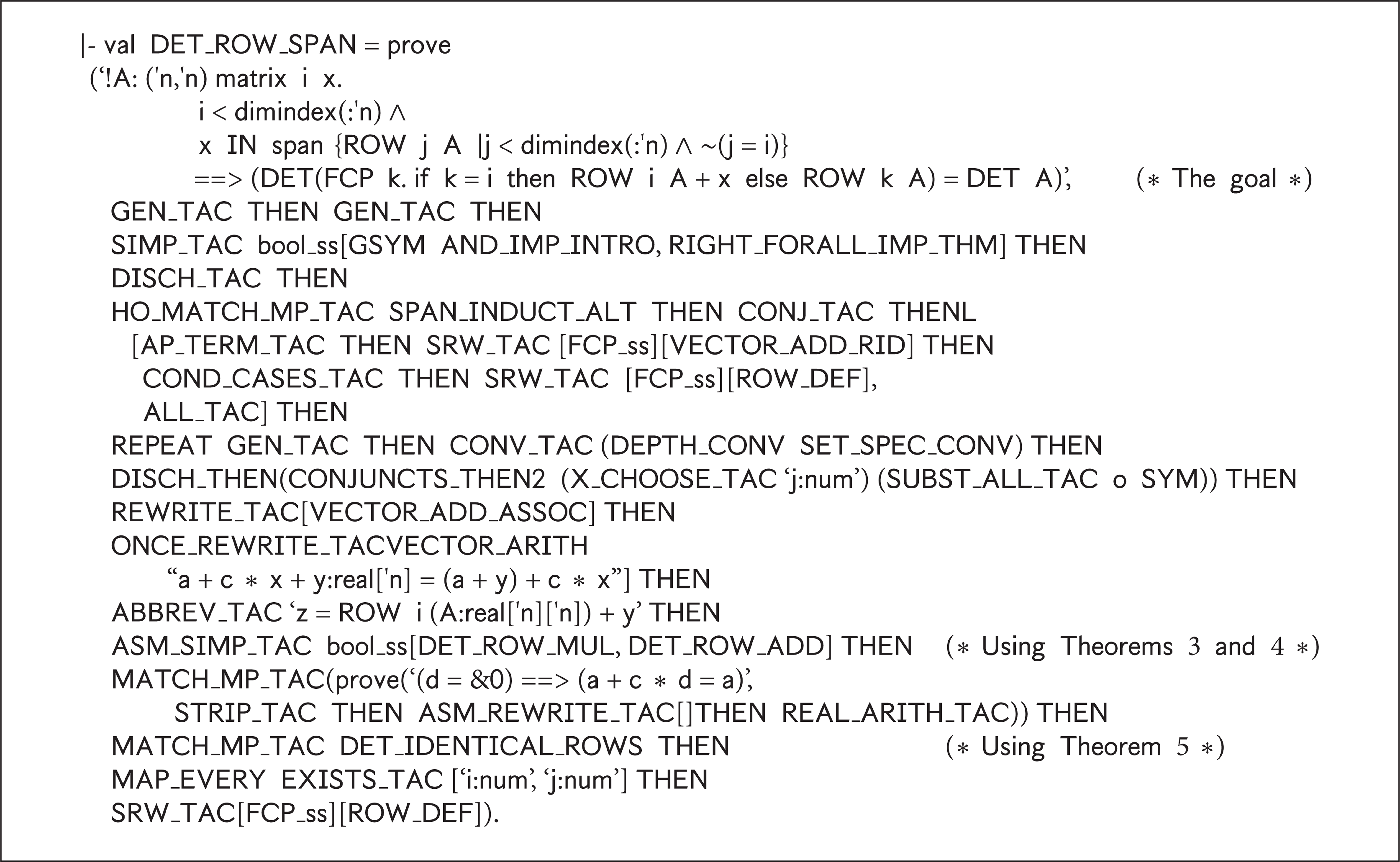
The proof of Theorem DET_ROW_SPAN.
To prove Theorem 7, the determinant of the new matrix, which is formed by adding linear combinations of rows of A into any one of the rows, is rewritten as a sum of the subdeterminants in accordance with Theorems 3 and 4. One of the matrices corresponding to the subdeterminants is matrix A, and the rest of corresponding matrices have duplicated rows. Then, Theorem 4 is employed to finish the proof.
4. Applications
In this section, two formal modeling and proving applications are presented, parameterized two-port networks and state transfer equations.
4.1. Parameterized Two-Port Networks
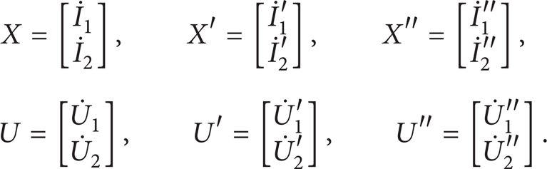
The behavior of many electronic components can be described by their characteristic matrices. Many complex passive and linear circuits can be modeled using a two-port network model [14], which is used to model an isolate portion of a larger circuit in mathematical circuit analysis techniques. Two-port networks can describe any linear circuit with four terminals provided that it does not contain an independent source and satisfies the port conditions. The examples include filters, matching networks, transmission lines, transformers, and small-signal models for transistors. It is meaningful to formally model a two-port network for formally modeling and verifying complex linear circuits. Here, we present the formal models of two-port networks. A two-port network is abstracted as a black box with four terminals: voltage U1 and current I1 at the input port and voltage U2 and current I2 at the output port. When any two of the four variables are given, the other two can always be derived by a certain 2 × 2 parameter matrix. Furthermore, when two or more two-port networks are connected, the parameters of the combined network can be calculated by performing matrix algebra on the parameter matrices of the component two ports.
Two-port networks can be connected in different ways. We verify two connecting styles: the cascade configuration as shown in Figure 1 and the parallel-parallel configuration as shown in Figure 2.
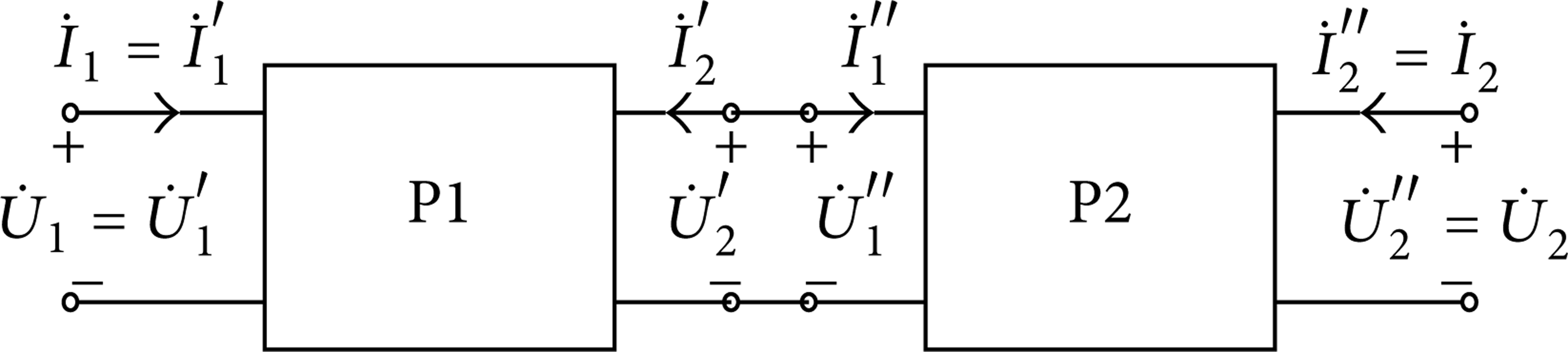
Two ports connected in a cascade connection.

The two ports connected in a parallel-parallel configuration.
When the two-port P1 and the two-port P2 are connected in a cascade configuration, they form a composite two-port network, as shown in Figure 1 with symbol definitions. Let the transmission parameters of P1 and P2 be matrices T′ and T″. The individual two-port networks are described as follows:

Let

For a cascade configuration,

We have

Let T be the parameter matrix of the composite two-port network; we can then make the following deduction:

Therefore, we have the relationship of the composite two-port parameter and the parameters of individual two ports connected in a cascade connection:

The mathematical process is formally verified in HOL4, as shown in Algorithm 6. The property is proved based on the definition of the multiplication of matrices and the theorem of the equality of vectors. Note that the “2” in the “2 vector” is a type, whose cardinality is 2.
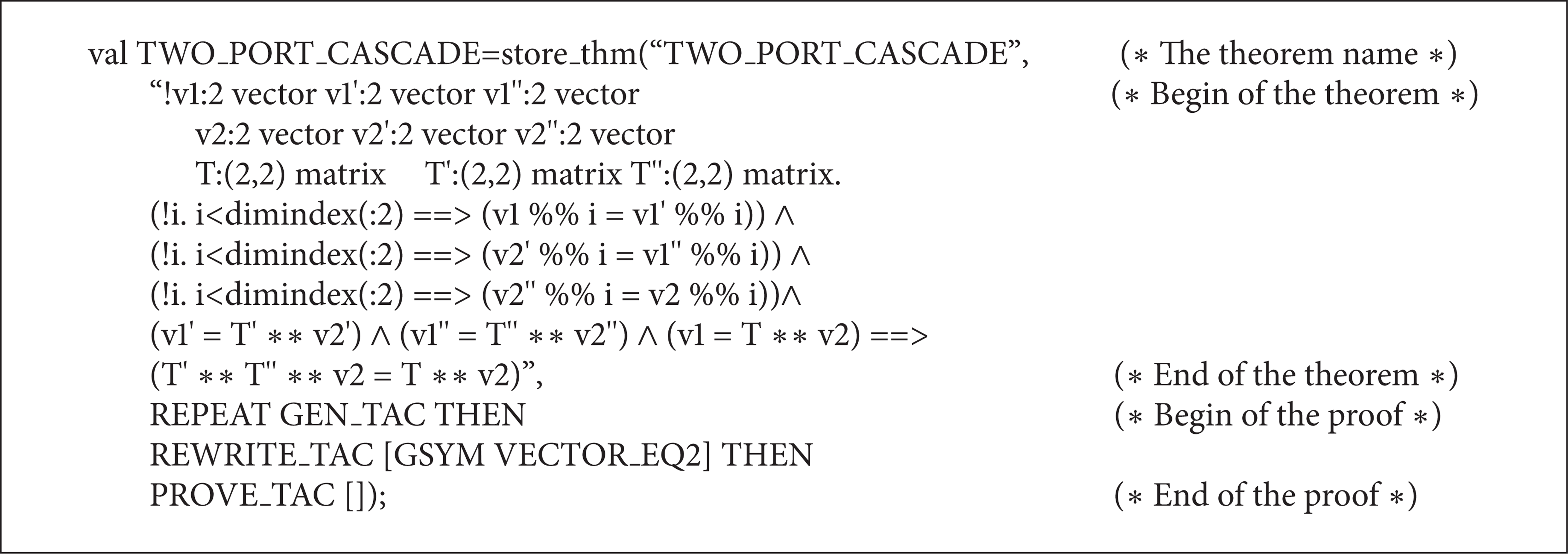
The proved HOL4 theorem of the property of a cascade connection of two ports.
Note that “v %% i” is used to replace “v ' i” simply to avoid confusion with superscripts “′” and “′′.” It can be seen from Algorithm 6 that the formalized vector and matrix are used to model the two-port network and its property, and the proof is very brief thanks to the formalized theory.
When two-port P1 and two-port P2 are connected in a parallel-parallel configuration, they form a composite two-port network, as shown in Figure 2 with symbol definitions. The input voltage and output voltage of the composite two-port networks equal that of the individual two ports, respectively; that is,

If each of the port conditions is not changed by the parallel connection, the current of the composite two-port networks is equal to the sum of the current of the component two ports:

Let
That is to say,

Let Y′ and Y″ be the y-parameter matrices of P1 and P2, respectively; then,

Let Y be the y-parameter matrix of the composite two-port network. We have

The equation shows that the y-parameters of the composite network are found by the matrix addition of the two individual y-parameter matrices of two ports connected in a parallel-parallel configuration; that is,

The above mathematic process is verified formally in HOL4, as shown in Algorithm 7.
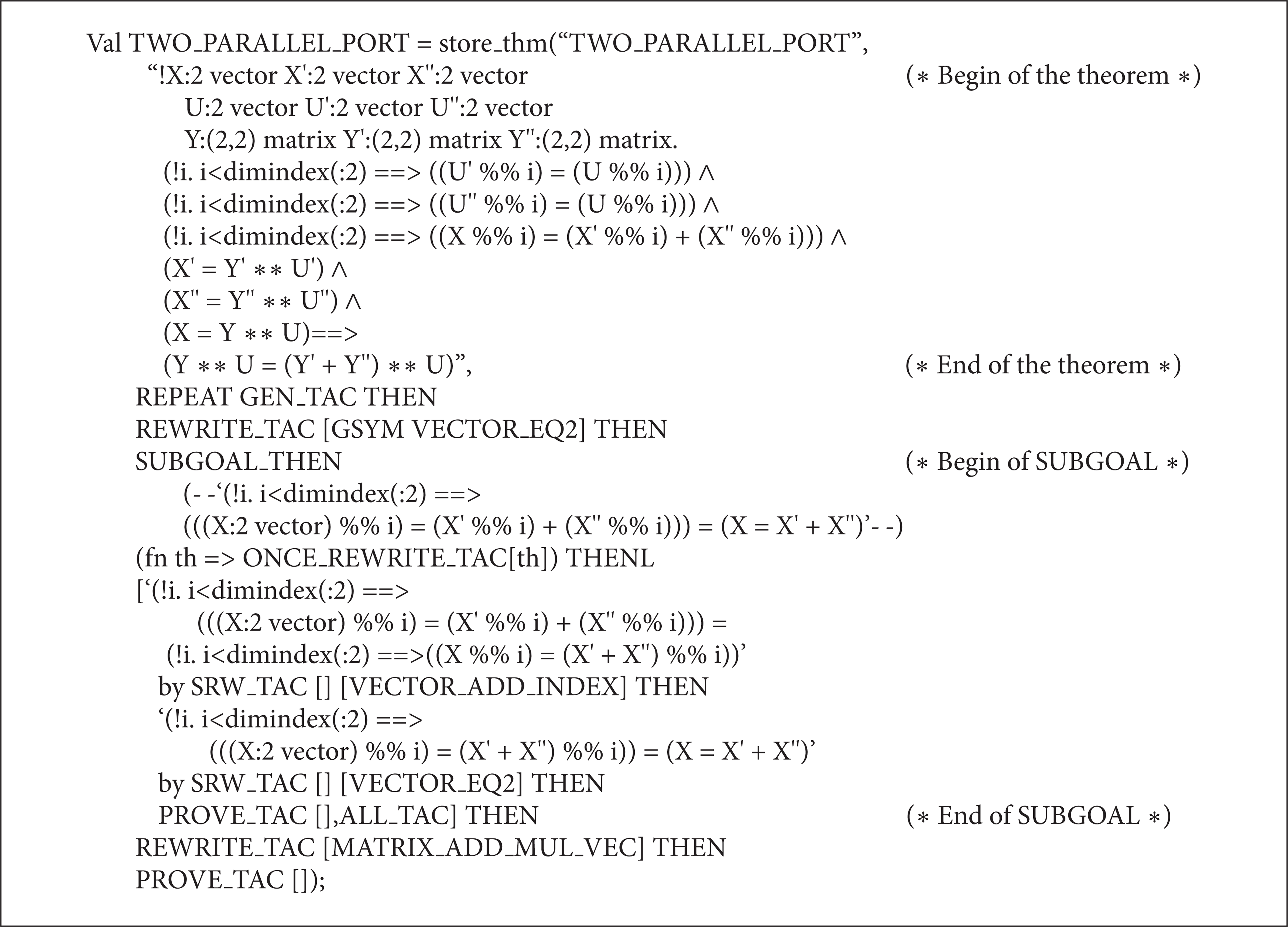
The proved HOL4 theorem of the property of a parallel-parallel configuration of two ports.
In the proof, a lemma “(!i. i<dimindex(:2) ==> ((X %% i) = (X′ %% i) + (X′′ %% i))) = (X = X′ + X′′),” which has not previously been proven, is needed; it is introduced as a subgoal. In addition, the theorem MATRIX_ADD_MUL_VEC is used to prove the goal.
4.2. State Transfer Equations
In this subsection, we present an example that the high-speed power of matrix is employed to solve state transfer equation problems, and the formalization and verification are illustrated. The problem is described as follows. There are p (2 ≤ p ≤ 1000000) lotus flowers in a lake and on one of the flowers there is a frog. The frog is capable of jumping from any flower to any other one. The frog can and must move from a flower it stays on to another flower by a jumping. If the frog starts to jump from a flower and comes back the same flower by n (2 ≤ n ≤ 231 − 1) jumping, how many jumping paths are there in all? The solution can be derived by iteration. Let f[n] denote the number of jumping paths by n jumping, and g[n] denotes the number of jumping paths from one flower to another. So, the iterations can be written as
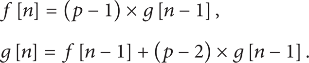
Consider (f[n] g[n]) as state vector on time n; then (f[n − 1] g[n − 1]) is state vector on time n − 1; the state transfer equation is

The solution is easy to be deduced iteratively as
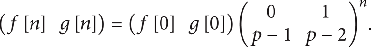
When n could be very large, the high-speed power of matrix is indispensable to compute the solution.
In general, many state transfer problems could be modeled by state transfer equations and the high-speed power of matrix can speed up computing the results. In the rest of the section, we formally prove that the state transfer equation could be solved by power of matrix and further prove that there is high-speed power of matrix speeding up computing the solution.
First, prove that if “

Induction proof of the solution by power of matrix for state transfer equation.
Second, prove that the solution can be computed by high-speed power of matrix. The solution by power of matrix could be derived by POW_M_INDUCT, and then the solution by high-speed power of matrix is verified. To prove this, the high-speed power of matrix is proved in advance. The proof is shown in Algorithm 9.

Proof of the solution by high-speed power of matrix for state transfer equation.
Third, the problem of the frog jumping could be formalized and verified by instantiating the above proof according to (22). The proof is shown in Algorithm 10.

Instantiating proof of the solution for the frog jumping problem.
5. Conclusions
Vectors and matrices are extensively used to model linear transformation of engineer and scientific problems. In this paper, the vector and matrix algebra, which are the fundamentals of linear system models, were formalized in the HOL4 theorem prover. Vectors and matrices were constructed based on the FCP library; then the properties of the operations of vectors and matrices were formally verified. The formalized vector and matrix theories help to extend the applications of HOL4. In order to illustrate the usefulness of the formalized matrix theory, we formally analyzed the behaviors of two kinds of composite two-port networks and high-speed power of matrix solution for state transfer equations. The proposed approach is able to offer exact results and is not subject to slip up. Our future work will focus on the formalization of properties of linear transformation and the function matrix in HOL4, and the formalized matrix analysis theories will be employed to model and verify linear systems in engineering and scientific domains.
Conflict of Interests
The authors declare that there is no conflict of interests regarding the publication of this paper.
Footnotes
Acknowledgments
This work was supported by the International Cooperation Program on Science and Technology (2010DFB10930 and 2011DFG13000), the National Natural Science Foundation of China (60873006, 61070049, 61170304, 61104035, 61373034, and 61303014), the Natural Science Foundation of the City of Beijing (4122017), the S&R Key Program of the Beijing Municipal Education Commission (KZ201210028036), and the Open Project Program of State Key Laboratory of Computer Architecture and the Open Project Program of Guangxi Key Laboratory Trusted Software.