Flow Measurement Model of Ultrasonic Flowmeter for Gas-Liquid Two-Phase Stratified and Annular Flows

Abstract

An error correction model for ultrasonic gas flowmeter was proposed to explore the potential of an ultrasonic flowmeter for metering gas-liquid stratified and annular flows. The gas and liquid mass flowrates could be obtained provided that the gas quality and physical prosperities were known. A single-path ultrasonic flowmeter was investigated and the error of the apparent volumetric flowrate was considered as mainly resulting from the shrinkage of the gas flow path due to the presence of a liquid phase. Fourteen void fraction models were selected for the stratified and annular flows and evaluated against experimental data. It was demonstrated that the root-mean-square error of the gas mass flowrate can be reduced from 19.0% to below 5% by employing either of Lockhart & Martinelli, Baroczy, Spedding & Chen, or Wallis void fraction models. Lockhart & Martinelli model is recommended due to its higher accuracy, simpler formulation, sounder theoretical support, and stronger immunity to pressure variation. The error correction model proposed in this work provides a basis for developing new combination measurement methods with an ultrasonic flowmeter as one component.

1. Introduction

Gas-liquid two-phase flow of low liquid loading attracts considerable attention due to its common occurrence in petroleum, nuclear, and chemical engineering. The natural gas usually exhibits as gas-liquid two-phase flow of low liquid loading under stratified or annular flow regime in transportation pipelines. It is still a challenge to measure the individual flowrate of the gas and liquid phases on line accurately. Currently the metering of natural gas flow still relies on the separation approach heavily [1]. In the separation approach the natural gas flow is separated first and then the gas/liquid flowrates are measured separately by traditional single-phase flowmeters, respectively. The metering uncertainty is affected by the separation efficiency significantly. In some cases a certain amount of liquid is carried into the gas line, resulting in gas-liquid two-phase flow again. Moreover, bulky and heavy separators are mandatory in the separation approach. The requirement for maintenance and space of separators poses severe problems to some applications like offshore platforms where the maintenance and space are quite expensive and limited. The development of nonseparation approaches is a highly desired undertaking [2, 3].

Based on the understanding of the flow characteristics of gas-liquid two-phase flows of low liquid loading and the reliable performance of single-phase flowmeters, most research has been focused on developing error correction models for single-phase flowmeters in the nonseparation approaches [4–6]. The traditional single-phase flowmeters can be grouped into three categories according to the type of the measured flow parameter: (a) velocity-type flowmeters by which the velocity is directly measured such as ultrasonic, electromagnetic, and cross-correlation flowmeters or the velocity is transformed into displacement, differential pressure (DP), rotational speed, and frequency signals measured through rotameter, DP-type, turbine, and vortex flowmeters; (b) mass-type flowmeters by which the mass flowrate is directly measured like Coriolis flowmeter; (c) volume-type flowmeters by which the volumetric flowrate is directly measured like roots flowmeter. Much work has been carried out on the abovementioned flowmeters, especially on the DP-type flowmeters [7–11], for measuring the gas-liquid two-phase flows. However, the throttling element of DP-type flowmeters introduces much disturbance to the flow field. The disturbance increases the complexity of the interaction between the gas/liquid two phases, which results in higher and unavoidable measurement uncertainties.

The ultrasonic flowmeter (USF) is of noncontact and noninvasive nature, which has triggered some pioneer efforts on developing USF for gas-liquid two-phase flows [12, 13]. To obtain more information from USF multipath designs were also employed. However, a series of issues arises with the usage of multipath, such as mutual influence among the sound paths, installation effects, and complicated calibration. In this work a single-path USF is investigated for metering gas-liquid two-phase flow of low liquid loading. The objective of this work is to explore the potential of a single-path USF by developing error correction methods for measuring gas-liquid two-phase flows with potential applications to wet natural gas.

2. Modelling for Ultrasonic Flowmeter

2.1. Working Principle of Ultrasonic Flowmeter

The ultrasonic flowmeter investigated in this work has a single sound path [14]. There are two probes (A and B) positioned oppositely across the diameter of the pipe as shown in Figure 1. The ultrasonic flowmeter is installed horizontally to ensure that the sound path is located in the horizontal plane through the pipe axis. The flow signal is determined by alternately measuring the transit time of an acoustic signal traveling from one sensor to the other, designated as t₁ and t₂:

$\begin{array}{c}{t}_{\mathrm{1}}=\frac{L}{C+V_{\text{Path}}\cos \theta }\\ t_{\mathrm{2}}=\frac{L}{C-V_{\text{Path}}\cos \theta },\end{array}$

(1)

where L is the length of the sound path, C is the speed of sound in stationary fluid, V_Path is the average velocity along the sound path, and θ is the angle between the sound path and the pipe wall (i.e., the flow direction). The transit times are measured and then the average velocity is calculated by

$V_{\text{Path}}=\frac{D}{\sin \left(\mathrm{2}\theta \right)}\left(\frac{\mathrm{1}}{t_{\mathrm{1}}}-\frac{\mathrm{1}}{t_{\mathrm{2}}}\right),$

(2)

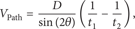
where D is the diameter of the pipe. A correction factor, K _U = V_Path/V, is often used to account for the effect of velocity profile when converting the average velocity along the sound path, V_Path, to the average velocity over the cross-sectional flow area, V.

Figure 1:

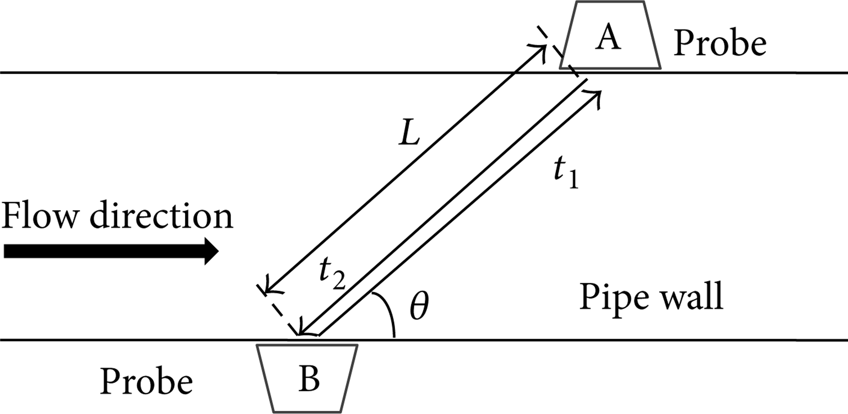
Illustration of the working principle of the ultrasonic flowmeter (top view for horizontal installation).

2.2. Modelling Stratified and Annular Flows

For the stratified flow with a low liquid level (as illustrated in Figure 2) the ultrasonic flowmeter essentially senses the flow of the gas phase only. This also applies to annular flows provided that the liquid film effect on the transit time measurement of the acoustic signal is negligible. Moreover, in this work the effect of the liquid flow on the velocity profile of the gas flow is not taken into consideration as an acceptable assumption. Thus the correction factor, K _U , used for the single-phase gas flow is also adopted for the gas flow in the two-phase flow case. The resultant error may be alleviated due to the low liquid loading discussed in this study. Based on the above simplifications it is considered that the error of the apparent gas flowrate mainly comes from the shrinkage of the gas flow path due to the existence of the liquid phase. Consequently the real gas volumetric flowrate can be obtained from the apparent flowrate through (3) with a known void fraction:

$\frac{Q_{\text{GU}}}{Q_{\text{G}}}=\frac{VA}{V{A}_{\text{G}}}=\frac{\mathrm{1}}{\alpha },$

(3)

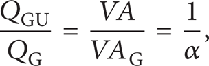
where Q_GU is the apparent gas volumetric flowrate from the ultrasonic flowmeter, Q_G is the real gas volumetric flowrate, V is the average velocity over the cross-sectional flow area, A is the cross-section area of the pipe, and α is the cross-sectional void fraction defined by

$\alpha =\frac{A_{\text{G}}}{A}=\frac{A_{\text{G}}}{A_{\text{G}}+A_{\text{L}}},$

(4)

where A_G and A_L are the areas on the cross-section of the pipe occupied by the gas and liquid phases, respectively. Substituting the void fraction into (3) the gas mass flowrate can be calculated by

$W_{\text{G}}={\rho }_{\text{G}}{Q}_{\text{GU}}\alpha ,$

(5)

where ρ_G is the gas density in the ultrasonic flowmeter.

Figure 2:

Schematic of the phase distribution of stratified flow in the ultrasonic flowmeter.

2.3. Selected Void Fraction Models

The published void fraction models can be grouped into four categories: (I) slip ratio model, (II) kα_H model, (III) drift flux model, and (IV) miscellaneous empirical model. In the present work a subset of the existing models of each category is selected based on the following criteria: (a) being applicable to separated flows (stratified flow and/or annular flow) in a circular tube, (b) being with only one unknown flow parameter, that is, the gas quality x (defined by (7)). Both superficial gas and liquid velocities are needed to be provided in the drift flux model; therefore, no drift flux models are included in this study. The homogeneous model is always presented for comparison. The basic assumption of the homogeneous model is that the liquid and gas phases travel at the same velocities. The homogeneous model is reasonably accurate for only a limited range of circumstances like bubbly and dispersed droplet or mist flows, where the entrained phase travels at almost the same velocity as the continuous phase.

2.3.1. Slip Ratio Models

The slip ratio is a concept used in separated flow models, where it is assumed that the two phases travel at two different mean velocities. Physically there cannot be a discontinuity in the two velocities at the interface since a boundary layer is formed in both phases on either side of the interface. Hence, the slip ratio is only a simplified description of relative mean velocities of the two coexistent phases. The slip ratio, S, is defined as

$S=\frac{U_{\text{G}}}{U_{\text{L}}}=\frac{{\rho }_{\text{L}}}{{\rho }_{\text{G}}}\frac{x}{\mathrm{1}-x}\frac{\mathrm{1}-\alpha }{\alpha },$

(6)

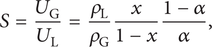
where ρ_L is the liquid density and U_G and U_L are the mean gas and liquid velocities, respectively. The gas quality, x, is the gas mass fraction of the two-phase flow:

$x=\frac{W_{\text{G}}}{W_{\text{TP}}}=\frac{W_{\text{G}}}{W_{\text{G}}+W_{\text{L}}},$

(7)

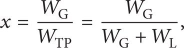
where W_TP is the total mass flowrate and W_G and W_L are the gas and liquid mass flowrates, respectively. Rearranging the expression of S the void fraction can be expressed using ρ_G/ρ_L, (1 − x)/x and S as follows:

$\alpha =\frac{\mathrm{1}}{\mathrm{1}+\left(\left(\mathrm{1}-x\right)/x\right)\left({\rho }_{\text{G}}/{\rho }_{\text{L}}\right)S}.$

(8)

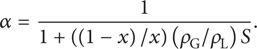
The void fraction models discussed here take the form of (8). The key of these void fraction models is to obtain the slip ratio under the condition that the gas quality, x, is known. Typical slip ratio models are discussed with emphasis on those applicable to stratified and annular flows as listed in Table 1. The variables μ_G and μ_L in the model equations below are dynamic viscosity of the gas and liquid phase, respectively.

Table 1:

Slip ratio models for void fraction.

Author/source	Index	Model equation
Homogeneous model	2	S = 1
Lockhart and Martinelli (1949) [15]	3	$S=\mathrm{0.28}{\left(\frac{\mathrm{1}-x}{x}\right)}^{-\mathrm{0.36}}{\left(\frac{{\rho }_{\text{G}}}{{\rho }_{\text{L}}}\right)}^{-\mathrm{0.64}}{\left(\frac{{\mu }_{\mathrm{L}}}{{\mu }_{\mathrm{G}}}\right)}^{\mathrm{0.07}}$
Zivi (1964) [16]	4	$S={\left(\frac{{\rho }_{\text{G}}}{{\rho }_{\text{L}}}\right)}^{-\mathrm{1}/\mathrm{3}}$
Baroczy (1966) [17]	5	$S={\left[\frac{\mathrm{1}-x}{x}\right]}^{-\mathrm{0.26}}{\left(\frac{{\rho }_{\text{G}}}{{\rho }_{\text{L}}}\right)}^{-\mathrm{0.35}}{\left(\frac{{\mu }_{\mathrm{L}}}{{\mu }_{\mathrm{G}}}\right)}^{\mathrm{0.13}}$
Smith (1969) [18]	6	$S=e+(\mathrm{1}-e){\left[\frac{{\rho }_{\text{L}}/{\rho }_{\text{G}}+e(\mathrm{1}-x)/x}{\mathrm{1}+e(\mathrm{1}-x)/x}\right]}^{\mathrm{0.5}},\mathrm{\hspace{0.17em}\hspace{0.17em}}e=\mathrm{0.4}$
Chisholm (1973) [19]	7	$S={\left[\mathrm{1}-x\left(\mathrm{1}-\frac{{\rho }_{\text{L}}}{{\rho }_{\text{G}}}\right)\right]}^{\mathrm{0.5}}$
Spedding and Chen (1984) [20]	8	$S=\mathrm{2.22}{\left[\frac{\mathrm{1}-x}{x}\right]}^{-\mathrm{0.35}}{\left(\frac{{\rho }_{\text{G}}}{{\rho }_{\text{L}}}\right)}^{-\mathrm{0.35}}$
Chen (1986) [21]	9	$S=\mathrm{0.18}{\left[\frac{\mathrm{1}-x}{x}\right]}^{-\mathrm{0.4}}{\left(\frac{{\rho }_{\text{G}}}{{\rho }_{\text{L}}}\right)}^{-\mathrm{0.67}}{\left(\frac{{\mu }_{\mathrm{L}}}{{\mu }_{\mathrm{G}}}\right)}^{\mathrm{0.07}}$
Hamersma and Hart (1987) [22]	10	$S=\mathrm{0.26}{\left[\frac{\mathrm{1}-x}{x}\right]}^{-\mathrm{0.33}}{\left(\frac{{\rho }_{\text{G}}}{{\rho }_{\text{L}}}\right)}^{-\mathrm{0.67}}$

2.3.2. Kα_H Models

The models listed in Table 2 calculate the void fraction through multiplying the homogeneous void fraction, α_H, by a coefficient, K:

$\begin{array}{c}{\alpha }_{\text{H}}=\frac{\mathrm{1}}{\mathrm{1}+\left(\left(\mathrm{1}-x\right)/x\right)\left({\rho }_{\text{G}}/{\rho }_{\text{L}}\right)}\\ \alpha =K{\alpha }_{\text{H}}.\end{array}$

(9)

Table 2:

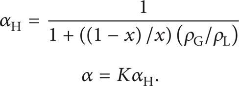
Kα_H models for void fraction.

Author/source	Index	Model equation
Homogeneous model	2	K = 1
Armand (1946) [23]	11	K = 0.833
Armand and Treschev (1947) [24]	12	K = 0.833 + 0.167x

2.3.3. The Miscellaneous Empirical Models

The miscellaneous empirical models derived from experimental data discussed in this paper are listed in Table 3.

Table 3:

The miscellaneous empirical models for void fraction.

Author/source	Index	Model equation
Wallis (1969) [25]	13	$\{\begin{array}{c}\alpha ={\left(\mathrm{1}+{X_{tt}}^{\mathrm{0.8}}\right)}^{-\mathrm{0.38}}\\ X_{tt}={\left[\frac{(\mathrm{1}-x)}{x}\right]}^{\mathrm{0.9}}{\left(\frac{{\rho }_{\text{G}}}{{\rho }_{\text{L}}}\right)}^{\mathrm{0.5}}{\left(\frac{{\mu }_{\text{L}}}{{\mu }_{\text{G}}}\right)}^{\mathrm{0.1}}\end{array}$
Huq and Loth (1992) [26]	14	$\alpha =\mathrm{1}-\frac{\mathrm{2}{(\mathrm{1}-x)}^{\mathrm{2}}}{\mathrm{1}-\mathrm{2}x+{\left[\mathrm{1}+\mathrm{4}x\left(\mathrm{1}-x\right)({\rho }_{\text{G}}/{\rho }_{\text{L}}-\mathrm{1})\right]}^{\mathrm{0.5}}}$
Cioncolini and Thome (2012) [27]	15	$\{\begin{array}{c}\begin{array}{c}\begin{array}{c}\begin{array}{c}\alpha =\frac{h{x}^n}{\mathrm{1}+(h-\mathrm{1})x^n}\\ h=-\mathrm{2.129}+\mathrm{3.129}{\left(\frac{{\rho }_{\text{G}}}{{\rho }_{\text{L}}}\right)}^{-\mathrm{0.2186}}\end{array}\\ n=\mathrm{0.3487}+\mathrm{0.6513}{\left(\frac{{\rho }_{\text{G}}}{{\rho }_{\text{L}}}\right)}^{\mathrm{0.5150}}\end{array}\\ \mathrm{0}<x<\mathrm{1},\hspace{0.17em}\mathrm{0.7}<\alpha <\mathrm{1},\hspace{0.17em}\mathrm{0.001}<\frac{{\rho }_{\text{G}}}{{\rho }_{\text{L}}}<\mathrm{1}\end{array}\\ \text{Annular\hspace{0.17em}flow}\end{array}$

3. Experiment

3.1. Test Facility

The experiment was conducted on the gas-liquid two-phase flow test facility at China University of Petroleum (Huadong) as sketched in Figure 3. The gas (air) is supplied by a screw compressor and fed into a receiver to attenuate the pressure fluctuations from the compressor. The liquid (water) is supplied by a centrifugal pump from a water tank. The gas and liquid flows are metered by a turbine flowmeter and Coriolis flowmeter with the maximum measured errors of 0.5% and 0.1% full scale, respectively. The desired gas/liquid flowrates are achieved by adjusting the valves downstream of the flowmeters. A T-shaped mixer is used to mix the gas and liquid two phases, then the gas-liquid two-phase mixture enters the flow loop with an internal diameter of 0.05 m. The flow loop consists of two sections: flow development section and test section. The total length of the flow loop is about 100 m with about 80 m and 20 m for the two sections, respectively. The tested ultrasonic flowmeter is located at the beginning of the test section. The gas-liquid two-phase flow returns to the water tank open to the atmosphere. Different pressures at the test section are achieved by choking the two-phase flow between the ultrasonic flowmeter and water tank. Pressure and temperature measurements are taken in the gas line, liquid line, and test section.

Figure 3:

Schematic of the gas-liquid two-phase flow test facility.

The tested ultrasonic flowmeter was manufactured by Endress + Houser with the model type of Proline Prosonic Flow B200 [14] for 2 inch pipelines. This single-path ultrasonic flowmeter is designed to measure the volumetric flowrate of gas flow and calibrated using air flow. The measuring range of the ultrasonic flowmeter is from 9 m³/h to 269 m³/h. The maximum relative error is from ± 3.0% for 9 m³/h to 26.9 m³/h and ± 1.5% for 26.9 m³/h to 269 m³/h with the repeatability of ± 0.5% of reading.

3.2. Test Condition and Flow Regime

The experiment was conducted under different system pressures including 0.2 MPa, 0.3 MPa, 0.4 MPa, and 0.5 MPa. The superficial gas and liquid velocities (U_SG and U_SL) range from 4 m/s to 30 m/s and from 0.01 m/s to 0.7 m/s, respectively. The corresponding gas flowrate ranges from 30 m³/h to 225 m³/h. The test points in terms of U_SG and U_SL are plotted on Taitel & Dukler flow regime map [28] as shown in Figure 4. All the test points fall into two regions in the flow regime map, that is, stratified flow and annular flows.

Figure 4:

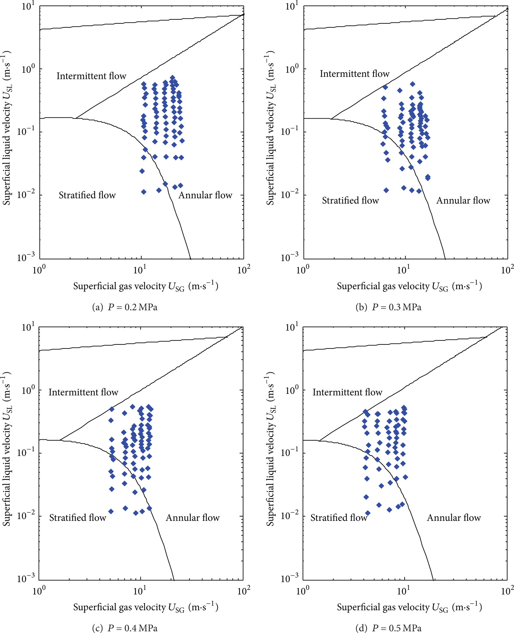
Test points plotted on Taitel & Dukler flow regime map [28].

4. Results and Discussion

4.1. Comparison among Void Fraction Models

The proposed error correction model (5) with different void fraction models is evaluated against experimental data. The gas mass flowrate is calculated based on the apparent reading from the USF and the performance of the void fraction models is assessed by the relative error and root-mean-square error defined by (10) and (11). The relative error, E _R , is expressed as

$E_R=\frac{W_{\text{Mod}}-W_{\text{Ref}}}{W_{\text{Ref}}}\times \mathrm{100}\%,$

(10)

where W_Mod and W_Ref are the gas mass flowrates calculated by the proposed error correction model and measured by the reference gas flowmeter in the experiment designated as the true flowrate, respectively. The root-mean-square error, E_RMS, is defined as

$E_{\text{RMS}}=\sqrt{\frac{{\sum }_{i=\mathrm{1}}^N{\left(E_{Ri}\right)}^{\mathrm{2}}}{N-\mathrm{1}}},$

(11)

where N is the total number of the test points and i is the index of the test point.

There are fifteen groups of E_RMS and maximum E _R (absolute value) for the gas mass flowrate calculation as presented in Figure 5 with Index of 1 to 15. The calculation of the gas mass flowrate without any correction is labeled as Index = 1 for comparison with the other models (Index = 2 to 15). Each group includes four points of E_RMS and maximum E _R representing the four tested pressures, that is, P = 0.2 MPa, 0.3 MPa, 0.4 MPa, and 0.5 MPa, respectively. It can be seen from Figure 5 that the E_RMS of the gas mass flowrate without any correction is as high as 22.6% and the maximum E _R is 60.1% at P = 0.5 MPa. The large errors due to the presence of the liquid phase are expected and show the great necessity to make corrections. Similarly the homogeneous model does not work well because the homogeneous flow assumption deviates far away from the real cases of horizontal stratified and annular flows since there is obvious velocity difference between the gas/liquid two phases. Both the resultant E_RMS and maximum E _R are lower than those without any correction; however, an E_RMS of 17.6% and maximum E _R of 43.9% at P = 0.5 MPa resulting from the homogeneous model are still significantly large. An error with E_RMS smaller than 10% can be obtained by employing the rest void fraction models with Index from 3 to 15.

Figure 5:

Root-mean-square errors and maximum relative errors of the gas mass flow rate for different void fraction models at different pressures. Index = 1: no correction model; Index = 2: the homogeneous model; Index = 3 to 10: slip ratio models; Index = 11 to 12: Kα_H models; Index = 13 to 15: the miscellaneous empirical models.

Four models of Lockhart & Martinelli, Baroczy, Spedding & Chen, and Wallis (Index = 3, 5, 8, and 13) have achieved a better performance with the E_RMS smaller than 5% and maximum E _R smaller than 20% at all the tested pressures. An average E_RMS among all the tested pressures has been reduced from 19.0% without any correction to 4.6%, 3.9%, 3.7%, and 4.0% with the above four void fraction models applied, respectively. The smallest average E_RMS has been obtained by Spedding & Chen model followed by Baroczy model; however, there is a much larger scatter in E_RMS due to the pressure effects than those of Lockhart & Martinelli and Wallis models. Spedding & Chen model was originally developed for annular flows and roll wave flows, which are similar to the test conditions in this work. However, no viscosity effect was taken into consideration by this model. It is believed that the viscosities affect the interaction forces at the interface between the two phases, slip ratio, and void fraction. Thus it is necessary to incorporate the viscosity effect into the void fraction models. The viscosity effect was included in Chen model later; however, the fact that the resultant E_RMS and maximum E _R of Chen model are even higher (E_RMS about 10% and maximum E _R about 30%) shows that the viscosity effect has not been dealt with properly. It is not surprising that Lockhart & Martinelli, Baroczy, and Wallis models have achieved similar performance, because all of them employed Lockhart-Martinelli number, X _tt , as a key model parameter essentially. The first X _tt -based void fraction model was proposed by Lockhart & Martinelli based on the separated flow model theory; Baroczy developed the void fraction model with X _tt and a property index (related to the viscosity and density) as model parameters; Wallis model is essentially a best fit for the data presented by Lockhart & Martinelli. X _tt was defined as the square root ratio of the liquid-only pressure gradient to the gas-only pressure gradient, through which all of the gas quality, density, and viscosity are taken into account. Generally the X _tt -based models have been widely used in stratified and annular flow cases by many researchers.

A similar average E_RMS and maximum E _R to those of Lockhart & Martinelli model have been obtained by Zivi model. Zivi model was proposed for annular flows with the assumptions that no liquid is entrained in the gas core and the total kinetic energy of the two phases tends to be minimized. The fraction of the liquid droplet entrainment in the gas core is introduced into Smith model, where the fraction, e, equals the mass flowrate of droplets divided by the total liquid mass flowrate. It is believed that the parameter e is affected by several factors such as flow velocities, fluid properties, and pipe diameter; thus a fixed value of e may result in errors for a wide range of flow conditions. The requirement for an appropriate evaluation of e poses a difficulty to the application and accuracy of Smith model. It is postulated that an improper treatment on the liquid entrainment contributes to the errors of Zivi and Smith models. Huq & Loth and Cioncolini & Thome models are dedicated annular flow models but were mainly applied to vertical upflows in the original works. However, the resultant errors are comparable to those of models developed for horizontal flows showing the strong robustness of Huq & Loth and Cioncolini & Thome models. It needs to be stressed that the above void fraction models as well as Chisholm, Armand, and Armand & Treschev models are not the preferred ones due to the lack of accounting for the viscosity effects.

The pressure effect on E_RMS is not consistent for all the presented void fraction models as can be observed in Figure 5. The void fraction models can be classified into four groups in terms of the pressure effect on the E_RMS: (a) little effect such as Lockhart & Martinelli, Smith, Chisholm, Wallis, and Huq & Loth; (b) more significant effect with the increase of the pressure, such as the homogeneous model, Chen, Hamersma & Hart, Armand, Armand & Treschev and Cioncolini & Thome; (c) less significant effect with the increase of the pressure, such as Zivi; (d) no consistent effect such as Baroczy and Spedding & Chen. Among all the discussed void fraction models there is a common variable, ρ_G, which is directly affected by the pressure. It is postulated that the performance of the void fraction models experiencing varying pressures can be improved through dealing with the term, ρ_G, properly.

4.2. Error Correction Model with Lockhart & Martinelli Model

Based on the above discussion in Section 4.1 it is recommended that Lockhart & Martinelli void fraction model should be employed in the error correction model (5) proposed in this work due to its higher accuracy, simpler formulation, more theoretical support, and stronger immunity to pressure variation. To highlight the performance of the error correction model with Lockhart & Martinelli void fraction model the relative error, E _R , is plotted against the gas quality, x, in Figure 6. For most of the test points E _R is located within ± 5%. There are mainly two sources for the model prediction errors.

1. Lockhart & Martinelli void fraction model has been adopted in the error correction model, where the uncertainty of this void fraction model itself introduces model prediction errors unavoidably.

2. Several simplifications have been made when developing the error correction model, which are also considered as important contributions to the model prediction errors.

Figure 6:

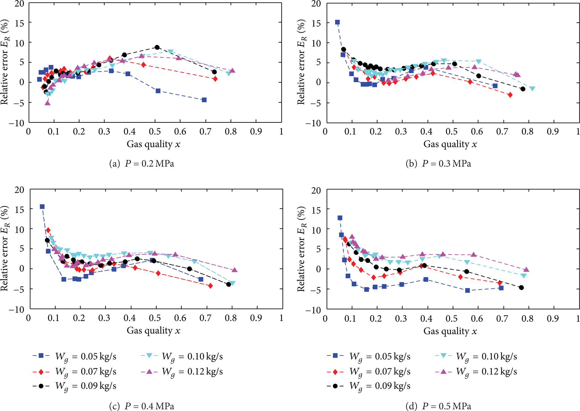
Relative error of gas mass flowrate for the error correction model with Lockhart & Martinelli void fraction model at different pressures.

A significantly larger E _R occurs at lower W_G and lower x for P = 0.3 MPa, 0.4 MPa, and 0.5 MPa, which is different from that for P = 0.2 MPa. The largest errors for P = 0.3 MPa, 0.4 MPa, and 0.5 MPa appear at the test points with the lowest W_G and the lowest x. The test points can be identified in the flow regime map (Figure 4). All of the three test points are located at the boundary between the annular flow and intermittent flow regions. The intermittent flows include plug flow and slug flow. The slug flow region is adjacent to the annular flow region. Thus it is postulated that the largest errors result from the intended flow regime transition between the annular flow and slug flow. Liquid waves with the void fraction less than 0.5 may appear now and then at the test section. The large liquid wave takes a significant portion of the sound path of the ultrasonic gas flowmeter resulting in a large velocity profile distortion as well as transit time measurement error. The flow conditions such as intermittent flows deviate too far away from those, based on which the proposed model is developed in Section 2.2. For the case of P = 0.2 MPa there is still a gap between the flow regime transition boundary and the test point with the lowest W_G and the lowest x showing that the annular flow remains. Thus no error as large as those for P = 0.3 MPa, 0.4 MPa, and 0.5 MPa has been obtained. Furthermore, it needs to be stressed that no obvious and consistent difference in E _R between the stratified flow and annular flow can be identified in Figure 6. This is not surprising when considering the annular flow under investigation occurs in a horizontal pipeline, where the liquid film on the upper part of the pipe wall is usually very thin compared with the liquid bulk at the bottom of the pipe due to gravity. Thus the horizontal annular flow with a high void fraction seems to be a similar case to the stratified flow.

5. Conclusions

Gas-liquid two-phase flows of low liquid loading in a horizontal pipeline usually exhibit stratified or annular flow regimes. It was proposed in this work to employ a gas ultrasonic flowmeter to measure the horizontal stratified or annular flows and a corresponding error correction model was developed. The gas and liquid mass flowrates could be obtained from the flow measurement model provided that the gas quality and physical prosperities were known. A single-path ultrasonic flowmeter was investigated and the error of the apparent volumetric flowrate was considered as mainly resulting from the shrinkage of the gas flow path due to the existence of the liquid phase. Fourteen void fraction models were selected for the stratified and annular flows first and then evaluated against experimental data collected in this work.

1. It was demonstrated that the root-mean-square error of the gas mass flowrate can be reduced from 19.0% to 4.6%, 3.9%, 3.7%, and 4.0% by employing void fraction models of Lockhart & Martinelli, Baroczy, Spedding & Chen, and Wallis, respectively, within the tested range of flow conditions.

2. Lockhart & Martinelli model is recommended due to its higher accuracy, simpler formulation, sounder theoretical support, and stronger immunity to pressure variation.

3. The proposed error correction model provides a basis for developing new combination methods for measuring the dual parameters of gas-liquid two-phase flows of low liquid loading with an ultrasonic flowmeter as one of the components.

Conflict of Interests

The authors declare that there is no conflict of interests regarding the publication of this paper.