Vehicle Optimal Velocity Curves for Minimum-Time Maneuver

Abstract

A problem in vehicle minimum-time maneuver is the assumption that a vehicle passes through a given path in a minimal amount of time without deviating from the boundary of the given path. Vehicle handling inverse dynamics provides a new perspective to solve such problem. Based on inverse dynamics, this paper transformed the problem of optimal vehicle velocity for minimum-time maneuver into that of optimal control with the objective function of minimum time. The path for minimum vehicle travel time and the optimal control model were established. The optimal velocity curves for three types of paths, namely, monotonically increasing path, monotonically decreasing path, and constant radius path, were analyzed. On this basis, the optimal velocity curves were solved for two kinds of concrete paths: a path of decreasing curvature radius followed by a path of increasing curvature radius and another path of increasing curvature radius followed by a path of decreasing curvature radius. Nine cases of possible optimal velocity curves were acquired. The optimal velocity curve of the given path, that is, a parabola followed by a semicircle, was obtained. Optimal velocity curves can be used as reference for vehicle minimum-time maneuver, which is an important issue for driver safety in fast-moving vehicles.

1. Introduction

A problem in vehicle minimum-time maneuver is the assumption that, without deviating from a given path boundary, a vehicle passes through a given path in a minimal amount of time [1]. This problem is difficult to solve with the use of open-loop and closed-loop methods in traditional handling dynamics. However, vehicle handling inverse dynamics provides a new perspective to solving the problem of minimum-time maneuver. Zhang et al. [2–4] examined the path-tracking problem with respect to vehicle handling inverse dynamics. Zhang and Pan [5] identified the steering wheel angle of a vehicle by using the inverse system method based on vehicle handling inverse dynamics. Casanova et al. [6–8] studied vehicle minimum-time maneuver by using a sequential quadratic programming algorithm to solve the constrained multivariable function minimum problem. Bunte et al. [9] studied the optimal slip angle under the tracking conditions of the given yaw rate. Bernard and Pickelmann [10] used optimal control method, under the condition of the given path, to calculate the input of the steering angle and braking force/driving force. By considering the lateral acceleration and longitudinal acceleration of a vehicle's centroid as the objective function, Hatwal and Mikulcik [11] repeatedly adopted the method proposed by Newton-Raphson in each time step to obtain the steering angle and braking force/driving force that would satisfy the requirements of the objective function. The results show that vehicle handling inverse dynamics can be studied using optimal control method. Hendrikx et al. [12] applied optimal control method to the inverse simulation of vehicle handling. This method required the establishment of an adjoint equation: a drawback of this method is the use of gradient descent method to solve the optimal control problem. Cossalter et al. [13] considered motorcycles as study objects to compute the path between two fixed points on the basis of the motorcycle's fastest speed. Basing on a nonlinear car model, Timings, and Cole [14] used convex programming to create a time-varying preview controller, optimized the steering wheel manipulation of a driver while maintaining the forward speed of a vehicle constant, and completed the travel path of a vehicle in a minimal amount of time. However, this study only considered the two freedom degrees of lateral and yaw and the nonlinearity of the tires to build the car model. Moreover, the algorithm for solving convex programming problem is too complex. In the case of maximum acceleration, Velenis and Tsiotras [15–18] used semianalytical methods to study the optimal velocity profile.

Basing on inverse dynamics, this research transformed the problem of optimal vehicle velocity for minimum-time maneuver into a problem of optimal control. In addition, on the basis of building the optimal control model, the optimal velocity curves were analyzed under the given monotonically increasing path, monotonically decreasing path, and constant radius path to solve the optimal velocity curves for two kinds of given paths: a path of decreasing curvature radius followed by a path of increasing curvature radius and another path of increasing curvature radius followed by a path of decreasing curvature radius. The optimal velocity curve of the given path, that is, a parabola followed by a semicircle, was obtained; this curve can be used as reference for the driver's minimum-time maneuver.

2. Optimal Control Model

2.1. Establishment of the Path

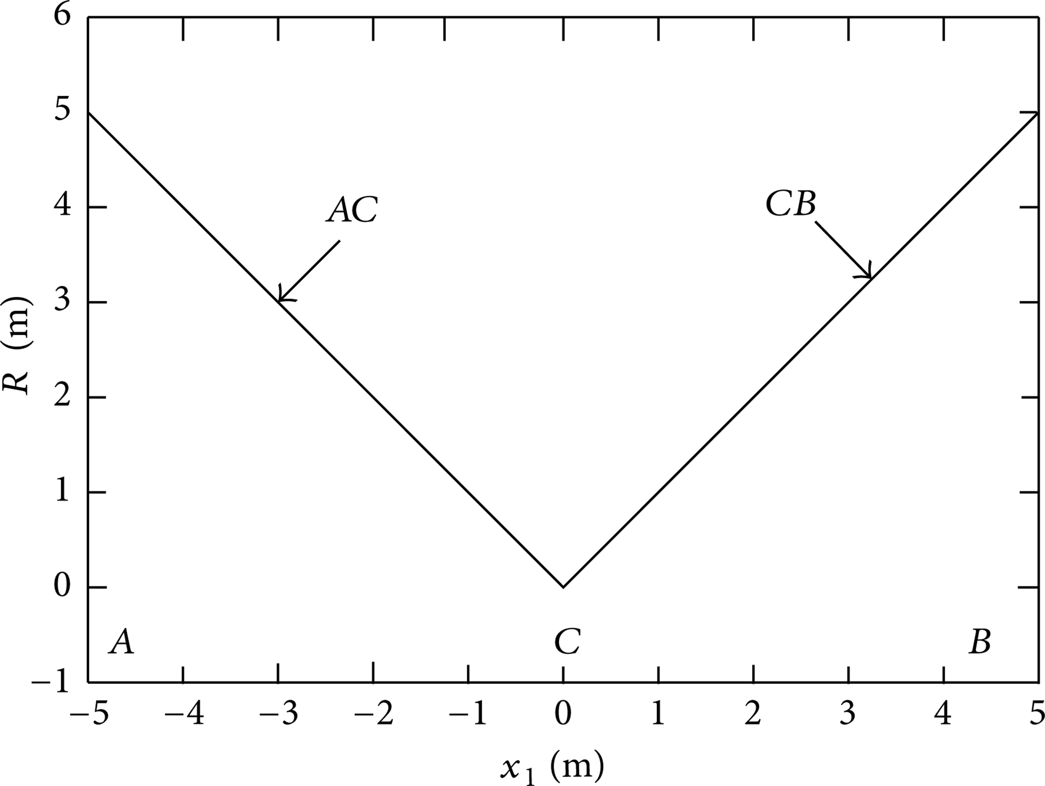
Significant parts of the race track are snake-shaped and u-shaped; thus, the studied path consists of a parabola, y₁ = − 0.2x² + 20x, and a semicircle, $y_{\mathrm{2}}=-\sqrt{\mathrm{256}-{(x-\mathrm{36})}^{\mathrm{2}}}$ , as shown in Figure 1. For convenience, the vehicle model is considered a moving particle with two degrees of freedom, and the studied path is a 2D curve.

Figure 1:

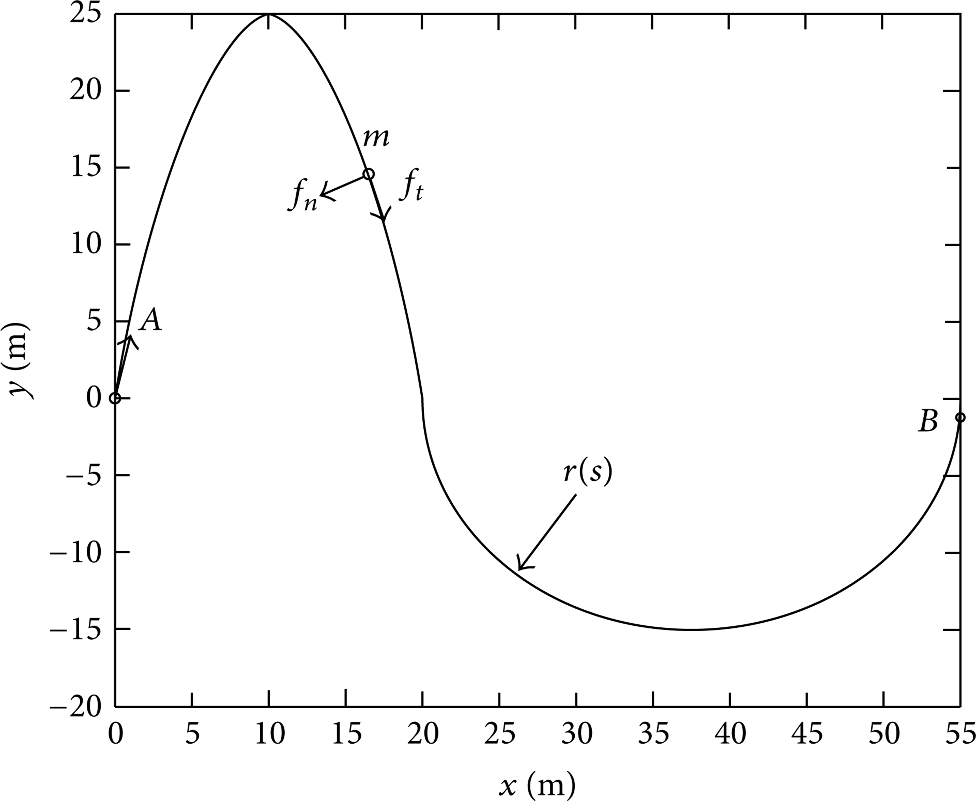
The profile of the given path.

2.2. Building of Optimal Control Model

The vehicle is simplified as a particle restricted by the given acceleration limits, the positions of initial point, the velocity of the initial point, and the final point, as shown in Figure 1. The given path is described by its radius at each point in the Cartesian coordinate system. Therefore, the system equation of motion can be obtained as follows [16]:

$m\frac{d^{\mathrm{2}}s}{d{t}^{\mathrm{2}}}=f_t,\hspace{1em}\hspace{1em}m{\left(\frac{ds}{dt}\right)}^{\mathrm{2}}=f_{n}r\left(s\right),$

(1)

where f _t is the tangential force along the path direction and f _n is the lateral force perpendicular to the path direction. Let $\alpha =\sqrt{m/F_{\max }}$ and β = αF_max/m. If τ = βt, x₁ = αβs, and x₂ = α(ds/dt), then f _t is the control input and F_max/m is the maximum acceleration limit. The control variable u is regarded as the optimal control variable in the minimum time to finish the given path in the control system. The constraint can be expressed as follows:

$\frac{f_t}{F_{\max }}=u\sqrt{\mathrm{1}-\frac{x_{\mathrm{2}}^{\mathrm{4}}}{R^{\mathrm{2}}\left(x_{\mathrm{1}}\right)}},\hspace{1em}u\in \left[-\mathrm{1},+\mathrm{1}\right],$

(2)

where R(x₁) = r(s).

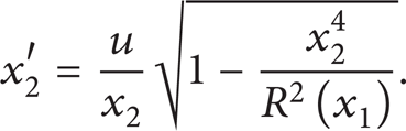
The state equation of the system is

${\dot{x}}_1=x_{\mathrm{2}},\hspace{1em}\hspace{1em}{\dot{x}}_2=u\sqrt{\mathrm{1}-\frac{x_{\mathrm{2}}^{\mathrm{4}}}{R^{\mathrm{2}}\left(x_{\mathrm{1}}\right)}},\hspace{1em}u\in [-\mathrm{1},+\mathrm{1}].$

(3)

To make (3) meaningful, we must satisfy the equation 1 − (x₂⁴/R²(x₁)) ≥ 0; that is, in the region S⊂R², the following should be defined:

$S=\left\{\left(x_{\mathrm{1}},x_{\mathrm{2}}\right):C_{\mathrm{0}}\left(x_{\mathrm{1}},x_{\mathrm{2}}\right)=x_{\mathrm{2}}^{\mathrm{2}}-\left|R\left(x_{\mathrm{1}}\right)\right|\le \mathrm{0}\right\}.$

(4)

Optimal control must be managed within the region S. On the boundary of S, the state is out of control.

The initial conditions are x₁₀ = x₁ and x₂₀ = x₂ at a time of τ = τ₀. The final value conditions are x_1f = x₁ and x_2f = x₂ at a time of τ = τ _f . Thus, the objective function of optimal control is $J={\int }_{{\tau }_{\mathrm{0}}}^{{\tau }_f}d\sigma$ . We suppose that the Hamiltonian function is expressed as follows:

$H\left(x,\lambda ,u\right)=\mathrm{1}+{\lambda }_{\mathrm{1}}{x}_{\mathrm{2}}+{\lambda }_{\mathrm{2}}u\sqrt{\mathrm{1}-\left(\frac{x_{\mathrm{2}}^{\mathrm{4}}}{R^{\mathrm{2}}\left(x_{\mathrm{1}}\right)}\right)},$

(5)

and the canonical equations of the system are

$\begin{array}{c}{\dot{\lambda }}_{\mathrm{1}}=-\frac{\partial H}{\partial x_{\mathrm{1}}}=-{\lambda }_{\mathrm{2}}u\frac{x_{\mathrm{2}}^{\mathrm{4}}}{\sqrt{\mathrm{1}-x_{\mathrm{2}}^{\mathrm{4}}/R^{\mathrm{2}}\left(x_{\mathrm{1}}\right)}}\frac{R^{\prime }\left(x_{\mathrm{1}}\right)}{R^{\mathrm{3}}\left(x_{\mathrm{1}}\right)},\\ {\dot{\lambda }}_{\mathrm{2}}=-\frac{\partial H}{\partial x_{\mathrm{2}}}=-{\lambda }_{\mathrm{1}}+\mathrm{2}{\lambda }_{\mathrm{2}}u\frac{x_{\mathrm{2}}^{\mathrm{3}}}{R^{\mathrm{2}}\left(x_{\mathrm{1}}\right)\sqrt{\mathrm{1}-x_{\mathrm{2}}^{\mathrm{4}}/R^{\mathrm{2}}\left(x_{\mathrm{1}}\right)}},\end{array}$

(6)

where R′(x₁) is the partial differential of the curvature radius to x₁; that is, $R^{\prime }(x_{\mathrm{1}})={\partial R(x_{\mathrm{1}})/\partial x}_{\mathrm{1}}$ . According to transversal condition, H(τ _f ) = 0 can be obtained. Moreover, the Hamiltonian function is not dependent on time; therefore, we have

$H\left(\tau \right)=\mathrm{0},\hspace{1em}\forall \tau \in \left[{\tau }_{\mathrm{0}},{\tau }_f\right].$

(7)

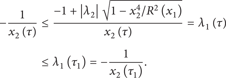
According to the principle of Pontryagin minimum, the optimal control variable can be obtained by

$u^{*}=\underset{u\in \left[-\mathrm{1},+\mathrm{1}\right]}{\text{argmin}}\hspace{0.17em}H\left(x,\lambda ,u\right)=\{\begin{array}{cc}-\mathrm{1},\hfill & {\lambda }_{\mathrm{2}}>\mathrm{0}\hfill \\ +\mathrm{1},\hfill & {\lambda }_{\mathrm{2}}<\mathrm{0}.\hfill \end{array}$

(8)

That is, u^*(τ) = − sgnλ₂(τ). Thus, λ₂ is a key function for determining the optimal control variable.

To achieve the minimum travel time of a vehicle at a given path, a vehicle must have the greatest and most effective driving force or braking force; that is, the optimal control variable u should always be in the control state of u = + 1 or u = − 1 in τ ∈ [τ₀, τ _f ] of the region S, and the movement of the vehicle is always traveling at maximum acceleration or maximum deceleration.

3. Analyses of Three Types of Cases in the Given Path

When the state equation (3) is in the proximity of the region boundary ∂S = {(x_α, x_β):C₀(x₁, x₂) = 0}, there is

$\frac{d{C}_{\mathrm{0}}\left(x_{\mathrm{1}},x_{\mathrm{2}}\right)}{dt}=\frac{\partial C_{\mathrm{0}}}{\partial x_{\mathrm{1}}}{\dot{x}}_{\mathrm{1}}+\frac{\partial C_{\mathrm{0}}}{\partial x_{\mathrm{2}}}{\dot{x}}_{\mathrm{2}}=-x_{\mathrm{2}}{R}^{\prime }\left(x_{\mathrm{1}}\right)\mathrm{sgn}R\left(x_{\mathrm{1}}\right).$

(9)

Therefore, the analyses can be performed in accordance with these three types of cases: (1) monotonically increasing path, in which the curvature radius of the travel trajectory gradually increases; that is, R′(x₁)sgnR(x₁) > 0; (2) monotonically decreasing path, in which the curvature radius of the travel trajectory gradually decreases; that is, R′(x₁)sgnR(x₁) < 0; and (3) constant radius path, in which the curvature radius of the travel trajectory is constant; that is, R′(x₁) = 0.

In the curved trajectory described by the curvature radius, when the limit of C₀(x₁, x₂) = 0 is met, a critical velocity can be set at the point of τ _c ∈ (τ₀, τ _f ), indicating that $x_{\text{2crit}}(x_{\mathrm{1}})=\sqrt{\left|R(x_{\mathrm{1}})\right|}$ . In x₂(τ _c ) = x_2crit(x₁(τ _c )), the tangential acceleration is equal to zero and ${\dot{x}}_{\mathrm{2}}({\tau }_c)=\mathrm{0}$ .

3.1. The Monotonically Increasing Path

For R′(x₁)sgnR(x₁) > 0, ${\dot{\lambda }}_1(\tau )\ge \mathrm{0}$ in τ ∈ [τ₀, τ _f ]. A critical point τ₁ ∈ (τ₀, τ _f ) is assumed to satisfy λ₂(τ₁) = 0. According to canonical equations, λ₁(τ₁) = − 1/x₂(τ₁) can be obtained, and in τ ∈ [τ₀, τ₁], there is

$-\frac{\mathrm{1}}{x_{\mathrm{2}}\left(\tau \right)}\le \frac{-\mathrm{1}+\left|{\lambda }_{\mathrm{2}}\right|\sqrt{\mathrm{1}-x_{\mathrm{2}}^{\mathrm{4}}/R^{\mathrm{2}}\left(x_{\mathrm{1}}\right)}}{x_{\mathrm{2}}\left(\tau \right)}={\lambda }_{\mathrm{1}}\left(\tau \right)\le {\lambda }_{\mathrm{1}}\left({\tau }_{\mathrm{1}}\right)=-\frac{\mathrm{1}}{x_{\mathrm{2}}\left({\tau }_{\mathrm{1}}\right)}.$

(10)

Equation (10) reveals that τ₁ is the critical point between u = + 1 and u = − 1.

If X _A ⁺(x₁) is defined as the forward integration of u = + 1 at (x₁ ^A , x₂ ^A ) for state equation (3) and X _B ⁻(x₁) is defined as the backward integration of u = − 1 at (x₁ ^B , x₂ ^B ) for state equation (3), then X _A ⁺(x₁) and X _B ⁻(x₁) can be used to describe the optimal velocity curve.

For the monotonically increasing path P _AB ⁺, there exists at most one critical point from u = + 1 to u = − 1 in the region S. Therefore, the optimal velocity curve can be expressed as follows:

$x_{\mathrm{2}}^{*}\left(x_{\mathrm{1}}\right)=\min \left\{X_A^{+}\left(x_{\mathrm{1}}\right),X_B^{-}\left(x_{\mathrm{1}}\right)\right\}\hspace{1em}{x}_{\mathrm{1}}\in \left[x_{\mathrm{1}}^A,x_{\mathrm{1}}^B\right].$

(11)

3.2. The Monotonically Decreasing Path

In the monotonically decreasing path, the optimal velocity curve is composed of the maximum acceleration and the maximum deceleration. Thus, a critical point from u = + 1 to u = − 1 exists in region S. In the following, we discussed the existence of the optimal velocity curve within region S. According to state equation (3), we have

$x_{\mathrm{2}}^{\prime }=\frac{u}{x_{\mathrm{2}}}\sqrt{\mathrm{1}-\frac{x_{\mathrm{2}}^{\mathrm{4}}}{R^{\mathrm{2}}\left(x_{\mathrm{1}}\right)}}.$

(12)

When u = − 1, $x_{\text{2min}}^{\prime }=-(\mathrm{1}/x_{\mathrm{2}})\sqrt{\mathrm{1}-(x_{\mathrm{2}}^{\mathrm{4}}/R^{\mathrm{2}}(x_{\mathrm{1}}))}$ . For the critical velocity $x_{\text{2crit}}(x_{\mathrm{1}})=\sqrt{\left|R(x_{\mathrm{1}})\right|}$ , $x_{\text{2crit}}^{\prime }(x_{\mathrm{1}})=R^{\prime }(x_{\mathrm{1}})\mathrm{sgn}R(x_{\mathrm{1}})/\mathrm{2}\sqrt{\left|R(x_{\mathrm{1}})\right|}$ . If $R^{\prime }(x_{\mathrm{1}})\mathrm{sgn}R(x_{\mathrm{1}})/\mathrm{2}\sqrt{\left|R(x_{\mathrm{1}})\right|}=\rho (x_{\mathrm{1}})$ , we have

$x_{\mathrm{2}}^{\mathrm{4}}+R^{\mathrm{2}}\left(x_{\mathrm{1}}\right){\rho }^{\mathrm{2}}\left(x_{\mathrm{1}}\right)x_{\mathrm{2}}^{\mathrm{2}}-R^{\mathrm{2}}\left(x_{\mathrm{1}}\right)\le \mathrm{0}.\mathrm{\hspace{0.17em}\hspace{0.17em}}$

(13)

When solving for x₂², because x₂ > 0, we have

$x_{\mathrm{2}}\le \sqrt{r_{\mathrm{2}}}\hspace{1em}={\left(\frac{-R^{\mathrm{2}}\left(x_{\mathrm{1}}\right){\rho }^{\mathrm{2}}\left(x_{\mathrm{1}}\right)+\sqrt{R^{\mathrm{4}}\left(x_{\mathrm{1}}\right){\rho }^{\mathrm{4}}\left(x_{\mathrm{1}}\right)+\mathrm{4}{R}^{\mathrm{2}}\left(x_{\mathrm{1}}\right)}}{\mathrm{2}}\right)}^{\mathrm{1}/\mathrm{2}}.$

(14)

Under a restrained condition that $x_{\text{2min}}^{\prime }=x_{\text{2crit}}^{\prime }$ , $x_{\text{2safe}}^{\prime }=\sqrt{r_{\mathrm{2}}}$ is obtained. The relation between x_2safe and x_2crit can be denoted by the followed equation:

$x_{\text{2safe}}^{\mathrm{4}}-x_{\text{2crit}}^{\mathrm{4}}+\left(\frac{{R^{\prime }}^{\mathrm{2}}\left(x_{\mathrm{1}}\right)}{\mathrm{4}}\right)x_{\text{2safe}}^{\mathrm{2}}{x}_{\text{2crit}}^{\mathrm{2}}=\mathrm{0}.\mathrm{\hspace{0.17em}\hspace{0.17em}}$

(15)

This finding indicates that x_2safe(x₁) < x_2crit(x₁) for all x₁ ∈ [x₁ ^A , x₂ ^B ], and x_2min′ > x_2crit′ between x_2safe and x_2crit.

For the monotonically decreasing path P _AB ⁻, at most one critical point from u = + 1 to u = − 1 exists in region S. Therefore, the optimal velocity curve can be presented as follows:

$x_{\mathrm{2}}^{*}\left(x_{\mathrm{1}}\right)=\min \left\{X_A^{+}\left(x_{\mathrm{1}}\right),X_B^{-}\left(x_{\mathrm{1}}\right)\right\}\hspace{1em}{x}_{\mathrm{1}}\in \left[x_{\mathrm{1}}^A,x_{\mathrm{1}}^B\right].$

(16)

3.3. The Constant Radius Path

The constant radius path is defined as C₀(x₁, x₂) = 0. In this study, vehicle velocity is considered the critical velocity. In this case, that is, f _n = F_max and ${\dot{x}}_{\mathrm{2}}=\mathrm{0}$ , the control input u does not reflect the velocity value, which is considered out of control. In other words, the tangential force cannot be generated. If force F_max is expressed as the lateral force, then R′(x₁) = 0 in this case.

Assume that C_ε(x₁, x₂) = x₂² + ε − |R(x₁)| = 0, where ε > 0 is a very small positive scalar, and when ε → 0, C₀(x₁, x₂) = 0. Through the calculation of the control limit, we have

$u_{sc}=\frac{R\left(x_{\mathrm{1}}\right)R^{\prime }\left(x_{\mathrm{1}}\right)}{\mathrm{2}\sqrt{\mathrm{2}\left|R\left(x_{\mathrm{1}}\right)\right|\epsilon -{\epsilon }^{\mathrm{2}}}}.\mathrm{\hspace{0.17em}\hspace{0.17em}}$

(17)

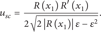
For random ε > 0, when R′(x₁) = 0, then u _sc ≡0.

For the constant radius path P _AB ⁰, the optimal velocity curve should include three parts: (1)X _A ⁺(x₁), which represents the forward integration of u = + 1 at (x₁ ^A , x₂ ^A ) for the state equation (3); (2) X _AF ⁰(x₁), in [x₁ ^A , x₁ ^F ], ε > 0, $x_{\mathrm{2}}(x_{\mathrm{1}})=\sqrt{\left|R(x_{\mathrm{1}})\right|-\epsilon }\le x_{\text{2crit}}(x_{\mathrm{1}})$ , and X _AF ⁰(x₁) consists of optimal control variable u = 0 and is consistent with u _sc in (17); that is R′(x₁) = 0; and (3) X _F ⁻(x₁), which denotes the backward integration of u = + 1 at (x₁ ^F , x₂ ^F ) for state equation (3).

The optimal velocity curve in the constant radius path is shown in Figure 2. At the phase of u = + 1, the vehicle begins to run at maximum acceleration from x₂(τ₀) = x₂ ^A . At the phase of u = 0, the vehicle runs at the maximum allowable velocity $\sqrt{\left|R(x_{\mathrm{1}})\right|-\epsilon }$ . At the phase of u = − 1, because X _F ⁻ is a terminal velocity, x₂(τ _f ) = x₂ ^F denotes backward integration at maximum deceleration. Combining the three phases, the optimal velocity curve in the constant radius path can be described as follows:

$x_{\mathrm{2}}^{*}\left(x_{\mathrm{1}}\right)=\min \left\{X_A^{+}\left(x_{\mathrm{1}}\right),X_{AF}^{\mathrm{0}}\left(x_{\mathrm{1}}\right),X_F^{-}\left(x_{\mathrm{1}}\right)\right\}.$

(18)

Figure 2:

The optimal velocity curve in the constant radius path.

4. The Optimal Velocity Curve

4.1. Application of the Optimal Velocity Curve

Two situations often occur in the actual path described by the curvature radius. One is a path of decreasing curvature radius followed by a path of increasing curvature radius, and the other is a path of increasing curvature radius followed by a path of decreasing curvature radius. On the basis of analysis of the optimal velocity curve for monotonically increasing and monotonically decreasing paths, the given path can be analyzed with respect to the two mentioned situations.

One path is assumed to be monotonically decreasing from A → C and another path is monotonically increasing from C → B, as shown as Figure 3. x₂^*(x₁) is used to denote the optimized velocity from A to B in the given path, and x₂ ^C* is the velocity of x₂^*(x₁) at pointC. According to the principle of Pontryagin minimum, if the velocity is optimal in A → B, then, in the first part A → C, the problem of minimum-time maneuver can be solved from the final condition x₂(τ _f ) = x₂ ^C* . Similarly, in the second part C → B, the problem of minimum-time maneuver can be solved from the initial condition x₂(τ _f ) = x₂ ^C* .

Figure 3:

The curve of the curvature radius of the given path of decreasing curvature radius followed by a path of increasing curvature radius.

If x₂ ^C* is not the optimal velocity, the problem of optimal velocity cannot consist of A → C and C → B. First, we must determine whether x₂ ^C* is the optimal velocity, which can be achieved by analyzing the critical point.

Part A → C belongs to the monotonically decreasing path, and according to the previous analysis possible optimal velocity curves include three cases, namely, u = + 1, u = − 1, and from u = + 1 to u = − 1, as described in Figures 4(a), 4(b), and 4(c), respectively. Similarly, part C → B is the monotonically increasing path, with possible optimal velocity curves for the three cases, namely, u = + 1, u = − 1, and from u = + 1 to u = − 1, as shown in Figures 4(d), 4(e), and 4(f), respectively.

Figure 4:

Possible optimal velocity curves of monotonically increasing path and monotonically decreasing path.

According to the principle of Pontryagin minimum, the overall path of A → B is composed of A → C and C → B; nine cases of optimal velocity curves exist, as shown in Figure 5.

Figure 5:

Nine cases of optimal velocity curves of the given path of the decreasing curvature radius followed by a path of increasing curvature radius.

For the first case, the optimal velocity curve is composed of the former u = + 1 and the latter u = + 1. The optimal velocity x₂^*(x₁) is the performance of X _A ⁺(x), and no other curve satisfies the boundary conditions of point A and point B. The velocity value of point C is less than or equal to x_2crit(x₁ ^C ). In this case, the optimal velocity x₂ ^C* depends on the boundary conditions of the point A and point B.

For the second case, the optimal velocity curve is composed of the former u = + 1 and the latter u = − 1, which differs from the first case. Other acceptable control critical points can be used to satisfy the boundary conditions of points A and B.

For the third case, the optimal velocity curve is composed of the former u = + 1, the latter u = + 1, and u = − 1. Similar to the first case, the entire curve has a turning point from acceleration to deceleration. However, because the boundary conditions of points A and B are not the same, the critical point is not point C.

For the fourth case, the optimal velocity curve is composed of the former u = − 1 and the latter u = + 1. Suppose that there is another optimal curve including a critical point to satisfy the boundary conditions of points A and B. If this curve is similar to that in the second case and the velocity is lowest at points A and B, then only when $x_{\mathrm{2}}^{C_{*}}=x_{\text{2crit}}(x_{\mathrm{1}}^C)$ can the optimal velocity curve be obtained, because point C is the moment out of control.

For the fifth case, the optimal velocity curve is composed of the former u = − 1 and the latter u = − 1. If the boundary conditions of points A and B are exchanged in the fifth case, its situation would become the same as the first case.

For the sixth case, the optimal velocity curve consists of the former u = − 1, the latter u = + 1, and u = − 1. Similar to the second case, other points of peak velocity aside from $x_{\mathrm{2}}^{C_{*}}=x_{\text{2crit}}(x_{\mathrm{1}}^C)$ satisfy the boundary conditions of points A and B.

For the seventh case, the optimal velocity curve consists of the former u = + 1, u = − 1, and the latter u = + 1. If the boundary conditions of points A and B are exchanged in the seventh case, its situation is the same as the sixth case.

For the eighth case, the optimal velocity curve consists of the former u = + 1, u = − 1, and the latter u = − 1. This curve is similar to that in the second and third cases, except that the critical point is located before point C.

For the ninth case, the optimal velocity curve consists of the former u = + 1, u = − 1, and the latter u = + 1 and u = − 1. Aside from $x_{\mathrm{2}}^{C_{*}}=x_{\text{2crit}}(x_{\mathrm{1}}^C)$ , other points of peak velocity satisfy the boundary conditions of the points A and B.

Analysis of these nine cases reveals the existence of two situations depending on the value of $x_{\mathrm{2}}^{C_{*}}$ . The first situation is that $x_{\mathrm{2}}^{C_{*}}\le x_{\text{2crit}}(x_{\mathrm{1}}^C)$ and $x_{\mathrm{2}}^{C_{*}}$ satisfy the boundary conditions of points A and B at the control turning point. The first, second, third, fifth, and eighth cases belong to this situation. The second situation is $x_{\mathrm{2}}^{C_{*}}=x_{\text{2crit}}(x_{\mathrm{1}}^C)$ ; that is, a control turning point exists at point C from u = + 1 to u = − 1. The fourth, sixth, seventh, and ninth cases belong to this situation.

For a path of increasing curvature radius followed by a path of decreasing curvature radius, based on the previous analysis, there are also 9 possible cases of optimal control.

However, for the fourth, sixth, seventh, and ninth cases, $x_{\mathrm{2}}^{C_{*}}=x_{\text{2crit}}(x_{\mathrm{1}}^C)$ at point C. The radius of point C is largest, so the velocity of the point C is largest in the curve A → B; that is,

$x_{\text{2crit}}\left(x_{\mathrm{1}}\right)<x_{\text{2crit}}\left(x_{\mathrm{1}}^C\right)\hspace{1em}{x}_{\mathrm{1}}\in \left[x_{\mathrm{1}}^A,x_{\mathrm{1}}^C\right)\cup \left(x_{\mathrm{1}}^C,x_{\mathrm{1}}^B\right].$

(19)

However, for the fourth, sixth, seventh, and ninth cases, assume that the velocity of the point C is minimum. There exists δ > 0, for x₁ ∈ (x₁ ^C − δ, x₁ ^C + δ), $x_{\mathrm{2}}^{C_{*}}<x_{\mathrm{2}}(x_{\mathrm{1}})$ . Due to $x_{\mathrm{2}}^{C_{*}}=x_{\text{2crit}}(x_{\mathrm{1}}^C)$ , we have x₂(x₁) > x_2crit(x₁) for x₁ ∈ (x₁ ^C − δ, x₁ ^C + δ). Thus the vehicle cannot run along the given path. Therefore, it can be inferred that the optimal velocity cannot appear in the fourth, sixth, seventh, and ninth cases. This means that the first, second, third, fifth, and eighth cases are considered reasonable.

4.2. The Optimal Velocity Curve of the Given Path

For the former section of the given path shown in Figure 1, that is the parabola y₁ = − 0.2x² + 20x, there are two cases which exhibit a monotonically increasing path and a monotonically decreasing path. According to the mentioned optimal control models and crucial point analyses, let u = + 1, and the vehicle is in a state of maximum acceleration within the limits. Based on (3), we have

${\dot{x}}_2=u\sqrt{\mathrm{1}-\frac{x_{\mathrm{2}}^{\mathrm{4}}}{R^{\mathrm{2}}\left(x_{\mathrm{1}}\right)}}=\sqrt{\mathrm{1}-\frac{x_{\mathrm{2}}^{\mathrm{4}}}{R^{\mathrm{2}}\left(x_{\mathrm{1}}\right)}}.$

(20)

Solving for the integral for velocity, we then arrive at

$x_{\mathrm{1}}=\mathrm{0.5}t{\left(\frac{R^{\mathrm{2}}{t}^{\mathrm{2}}}{R^{\mathrm{2}}+t^{\mathrm{2}}}\right)}^{\mathrm{1}/\mathrm{4}}.$

(21)

We plotted the velocity curves of $x_{\text{2crit}}(x)=\sqrt{\left|R(x)\right|}$ and $x_{\text{2safe}}(x)=\sqrt{r_{\mathrm{2}}(x)}$ and the relationship curve between velocity x₂ and displacement x₁ and put those in a figure. The preliminary curve of the optimal velocity for the former section of the give path can be obtained, as shown in Figure 6. It can be seen that optimal velocity is less than or equal to crucial velocity. In the segment A → B, the vehicle begins from point A and accelerates towards point B at the maximum acceleration (u = + 1). The vehicle decelerates in segment B → C (u = − 1) because the curvature radius of the path continuously decreases. This is in order to avoid sideslip, drift, and so on. From point C, the curvature radius begins to continuously increase, so the vehicle accelerates in the segment C → D (u = + 1). However, the latter section of the given path is semicircular in shape and the curvature radius decreases sharply at the junction. Therefore, the vehicle must decelerate before reaching point D in Figure 6, which is the embodiment of integrated maximum acceleration and boundary conditions, as shown in Figure 7.

Figure 6:

The preliminary curve of optimal velocity for the former section of the given path.

Figure 7:

The curve of optimal velocity for the former section of the given path.

The latter section with semicircle $y_{\mathrm{2}}=-\sqrt{\mathrm{256}-{(x-\mathrm{36})}^{\mathrm{2}}}$ is the path of the constant curvature radius (the curvature radius is 16). According to (20) and (21), the relationship between velocity x₂ and displacement x₁ can be obtained with the elimination of the variable t, and then the optimal velocity curve for the latter section semicircle can be acquired as shown in Figure 8. It can be observed that the vehicle is in acceleration phase (u = + 1) from the beginning. When $x_{\text{2crit}}(x)=\sqrt{\left|R(x)\right|}$ , the velocity does not change, and then the optimal velocity profile changes to a deceleration phase (u = − 1), and the velocity at the final point B becomes zero.

Figure 8:

The curve of optimal velocity for the latter section of the semicircle of the given path.

Based on the above analysis of optimal velocity curves, by combining Figures 7 and 8, the optimal velocity curve of the given path can be obtained, as shown in Figure 9. This optimal velocity curve can help drivers choose the best driving route with a reference value.

Figure 9:

The curve of optimal velocity for the given path.

5. Conclusions

The problem of optimal velocity for minimum-time maneuver was transformed into a problem of optimal control. On the basis of the optimal control model, the optimal velocity curves for monotonically increasing path, monotonically decreasing path, and constant radius path were analyzed. The optimal velocity curves were solved for two kinds of concrete paths: a path of decreasing curvature radius followed by a path of increasing curvature radius and another path of increasing curvature radius followed by a path of decreasing curvature radius. In consideration of the snake-shape and the u-shape of the race track as the given path, the corresponding optimal velocity curves were gathered. These optimal velocity curves can be used as reference for drivers running in the given path with a minimum amount of time. However, because the race track was simplified as a 2D curve, the obtained optimal velocity may be not accurate. In future studies, the race track can be modeled and simulated by 3D software to acquire more effective analyses.

Conflict of Interests

The authors declare that there is no conflict of interests regarding the publication of this paper.