Distributed Vector Quantization over Sensor Network

Abstract

A vector quantizer is a system for encoding the original data to reduce the bits needed for communication and storage saving while maintaining the necessary fidelity of the data. Signal processing over distributed network has received a lot of attention in recent years, due to the rapid development of sensor network. Gathering data to a central processing node is usually infeasible for sensor network due to limited communication resource and power. As a kind of data compression methods, vector quantization is an appealing technique for distributed network signal processing. In this paper, we develop two distributed vector quantization algorithms based on the Linde-Buzo-Gray (LBG) algorithm and the self-organization map (SOM). In our algorithms, each node processes the local data and transmits the local processing results to its neighbors. Each node then fuses the information from the neighbors. Our algorithms remarkably reduce the communication complexity compared with traditional algorithms processing all the distributed data in one central fusion node. Simulation results show that both of the proposed distributed algorithms have good performance.

1. Introduction

Vector quantization is one of data compression methods, encoding information by fewer bits than the original representation to reduce the communication and storage burdens, while maintaining the necessary fidelity of the data. A vector quantizer is a system of mapping input vectors into corresponding reproduction vectors drawn from a finite reproduction alphabet. There are two kinds of vector quantization algorithms. If each input is encoded using a certain rule that is independent of previous inputs or outputs, the vector quantization algorithm is classified as a memoryless method, like the LBG algorithm and tree-searched vector quantization [1–3]. Another kind of algorithms are called feedback vector quantization algorithms, incorporating memory into quantizer in choosing different codebooks for each input, like the vector predictive quantization [4, 5]. In this paper, we consider the memoryless ones.

In sensor network, sensors are distributed over a wide-range area. The data collected by different sensors are often different because sensors are at different locations under different environments. So information from all sensors is needed to obtain the overall data structure. Each sensor is a small device with limited power. To process data, traditional signal processing algorithms need all data available at a central processor, which is infeasible for distributed sensor network because the sensors cannot afford large data communication to gather all the data to one fusion node. Therefore, distributed algorithms, which need less communication, are needed in signal processing over sensor network. In recent years, many distributed algorithms are proposed, such as the distributed estimation algorithms [6–10], distributed detection algorithms [11, 12], and distributed clustering algorithms [13–15]. These distributed algorithms deal with the information extraction from spatially distributed nodes and fulfill the processing task based on the local computations and information from the nodes' neighbors. Nodes only transmit necessary parameters to their nearest neighbors instead of gathering the whole data set to one fusion node, so as to reduce the communication complexity and provide better flexibility and robustness to node/link failures. Applications of distributed signal processing algorithms in environmental monitoring, military surveillance, and source localization and extraction have been promoted in recent years [16–19].

In this paper, we consider distributed vector quantization. When using a sensor network as an exploratory infrastructure, we need to transmit and store the data collected by sensors. With a well-designed vector quantizer, fewer bits are needed for the communication and storage. Vector quantization will be certainly beneficial for the following data processing. Therefore, for distributed sensor network, vector quantization is needed. The goal of this paper is to design distributed vector quantization algorithms, which do not need to transmit all the data to a fusion center. LBG [20] and SOM [21] algorithms are two of the most popular methods among the vector quantization algorithms. These two methods are both basic algorithms and many modified algorithms based on LBG and SOM are proposed to achieve better performance. Based on the basic methods, LBG and SOM, here we present two distributed vector quantization algorithms, distributed LBG algorithm, and distributed SOM algorithm. Other modified algorithms based on traditional LBG and SOM can be easily extended to distributed version by applying our distributed process.

The rest of this paper is organized as follows. In Section 2, we briefly introduce the vector quantization problem and describe the distributed vector quantization problem. Our distributed LBG algorithm is presented in Section 3 and distributed SOM in Section 4. We present the numerical experimental results in Section 5. Finally, we draw conclusions in Section 6.

2. Preliminary Knowledge

2.1. Traditional Vector Quantization

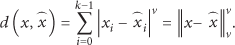
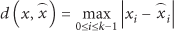
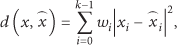
Mathematically, an N-level k-dimensional vector quantizer is a mapping, q, from each k-dimensional input vector, $x=(x_0,\dots ,x_{k-1})$ , to a reproduction vector, $\stackrel{⌢}{x}=q(x)$ , which is drawn from a finite reproduction alphabet, $\stackrel{⌢}{A}=\{y_i;\hspace{0.17em}i=1,\dots ,N\}$ . A vector quantizer is specified by the reproduction alphabet $\stackrel{⌢}{A}$ together with the partition, $S=\{S_i;\hspace{0.17em}i=1,\dots ,N\}$ , while $S_i$ refers to the input vector space, in which input vectors are mapped into the ith reproduction vector, $S_i=\{x:q(x)=y_i\}$ . The performance of a vector quantizer algorithm is measured by the total distortion between input vectors and their corresponding reproduction vectors, $D(q)=\sum d(x,\stackrel{⌢}{x})$ . The nonnegative distortion measure $d(x,\stackrel{⌢}{x})$ has several forms, in which the most common form for reasons of mathematical convenience is the squared-error distortion:

$$\begin{array}{cc}& d\left(x,\stackrel{⌢}{x}\right)={{\displaystyle \sum }}_{i=0}^{k-1}{\left|x_i-{\stackrel{⌢}{x}}_i\right|}^2.\end{array}$$

(1)

Other common distortion measures include the $l_v$ norm distortion

$$\begin{array}{cc}& d\left(x,\stackrel{⌢}{x}\right)={\left\{{{\displaystyle \sum }}_{i=0}^{k-1}{\left|x_i-{\stackrel{⌢}{x}}_i\right|}^v\right\}}^{1/v}\triangleq {\parallel x-\stackrel{⌢}{x}\parallel }_v\end{array}$$

(2)

and its vth power

$$\begin{array}{cc}& d\left(x,\stackrel{⌢}{x}\right)={{\displaystyle \sum }}_{i=0}^{k-1}{\left|x_i-{\stackrel{⌢}{x}}_i\right|}^v={\parallel x-\stackrel{⌢}{x}\parallel }_v^v.\end{array}$$

(3)

In addition, there are other distortion measures, like the $l_{\infty }$ norm distortion

$$\begin{array}{cc}& d(x,\stackrel{⌢}{x})=\underset{0\le i\le k-1}{\max }\left|x_i-{\stackrel{⌢}{x}}_i\right|\end{array}$$

(4)

and the weighted-squares distortion

$$\begin{array}{cc}& d\left(x,\stackrel{⌢}{x}\right)={{\displaystyle \sum }}_{i=0}^{k-1}{w}_i{\left|x_i-{\stackrel{⌢}{x}}_i\right|}^2,\end{array}$$

(5)

where $w_i\ge 0$ , $i=0,\dots ,k-1$ is the weight value. These distortion measures all depend on the vectors x and $\stackrel{⌢}{x}$ only through the error vector $x-\stackrel{⌢}{x}$ and such measures are called difference distortion measures.

2.2. Distributed Quantization Problem over Sensor Network

When it comes to a large-scale network, we need a distributed vector quantization algorithm as the traditional vector quantization algorithm is infeasible due to the difficulty of gathering all the data to a central processor. We consider the distributed quantization problem over a sensor network. The graphical representation of distributed vector quantization problem is shown in Figure 1. Each node collects its own input vectors and the goal of distributed vector quantization is to obtain the overall reproduction alphabet. The network is a connected graph with no isolated node. Each node collects its own data which may be unbalanced so that the data of one node cannot reflect the data structure of all the data of the network. We assume that each node can only communicate with its one-hop neighbors and the message delivery is reliable with little time delay. We consider an N-level k-dimensional vector quantizer over sensor network. Let J denote the number of nodes in the network, let $L_j$ denote the number of input vectors of node j, and ${\Gamma }^j$ denotes the set of neighbors of node j. The k-dimensional vector $x_l^j$ represents the lth input vector of the node j, and $X^j=\{x_l^j,l=1,\dots ,L_j\}$ represents the set of input vectors of node j. The k-dimensional vector $y_i^j$ represents the reproduction vector for ith partition of the node j in intermediate steps, and ${\stackrel{⌢}{A}}^j=\{y_i^j;i=1,\dots ,N\}$ represents the reproduction alphabet for node j in intermediate steps. After distributed vector quantization, we should obtain an overall reproduction alphabet $\stackrel{⌢}{A}=\{y_i;i=1,\dots ,N\}$ for the whole network.

Figure 1

The graphical representation of distributed vector quantization problem.

3. Distributed LBG Algorithm

3.1. LBG Algorithm

Here, we make a brief description of the well-known LBG algorithm [20]. The LBG algorithm aims to find the reproduction alphabet and the corresponding partition to minimize the expected distortion. The LBG algorithm is realized by a three-step loop. Given the initial reproduction alphabet ${\stackrel{⌢}{A}}_0$ , the iteration m does the following.

• (1)

For each input vector x, find the nearest reproduction vector $y_i$ in reproduction alphabet and assign x to partition $S_i$ :

$$\begin{array}{cc}& x\in S_i\hspace{1em}\text{only}\hspace{0.17em}\hspace{0.17em}\text{if}\hspace{0.17em}\hspace{0.17em}d\left(x,y_i\right)\le d\left(x,y_j\right),\hspace{0.17em}\hspace{0.17em}\forall j.\end{array}$$

(6)

(2)

If the total distortion between the input vectors and their corresponding reproduction vectors of the mth iteration, $D_m$ , is sufficiently close to that of the $(m-1)$ th iteration, $D_{m-1}$ , that is, $(D_{m-1}-D_m)/D_m\le \epsilon$ , end the loop, and use the ${\stackrel{⌢}{A}}_m$ together with S to describe the vector quantizer. Otherwise, continue.

(3)

For each partition $S_i$ , update the new reproduction vector $y_i$ as the centroid of $S_i$ :

$$\begin{array}{cc}& \underset{y_i}{\min }\hspace{0.17em}E\left(d\left(x,y_i\right)\mid x\in S_i\right).\end{array}$$

(7)

 

Replace m by   $m+1$ and go to step-1.

In step-1, we choose the minimum distortion reproduction vector for each input. By this step, we get the optimum partition for the current reproduction alphabet as (6). In step-2, we check the ending condition. Alternatively, we can check whether the partitions between two iterations are changed because the same partitions mean $D_m-D_{m-1}=0$ . In step-3, we get the centroid of each partition to minimize the distortion in each partition as (7). These steps guarantee that the total distortion is nonincreasing during the loops and we can always get a local optimal solution.

3.2. Distributed LBG Algorithm

The traditional LBG requires that all data are available in a central processor and can be accessed in their entirety during each iteration. When the data are distributed over the network and the communication ability of the sensor network is limited, we need a new distributed algorithm to solve the distributed vector quantization problem. Here, we put forward our distributed LBG algorithm. In brief, each node, in our algorithm, executes several inner loops of a modified traditional LBG and then transmits the local results, the reproduction alphabet and the corresponding partition counts denoted as ${\stackrel{⌢}{A}}^{\prime }=\{y_i^{\prime },\hspace{0.17em}i=1,\dots ,N\}$ and $B=\{n_i,\hspace{0.17em}i=1,\dots ,N\}$ , to its neighbors in outer loops. Each node receives messages from neighbors. Then each node updates the new reproduction vectors by fusing its local results with the messages from its neighbors. The outer loops continue until convergence. After all nodes stop outer loops, we collect all the local results to get the final reproduction alphabet. Our idea for distributed LBG algorithm is borrowed from the distributed k-means clustering [13]. k-means algorithm is similar to LBG algorithm in philosophy. Clustering wishes to group existing data while quantization wishes to find the data structure and uses it on future data. Here, we modify the distributed k-means algorithm for vector quantization, doing some modification for reduction in communication complexity and improvement in distortion performance. The detailed explanation is given as follows.

At the beginning of our distributed LBG algorithm, we generate the initial reproduction alphabet ${\stackrel{⌢}{A}}_0$ along with a termination threshold ϵ for all nodes in the network. Set $m=1$ and start the loops. For node j in iteration m of outer loop, the algorithm is carried out as follows. First of all, we execute p inner loops of the three-step-loops of traditional LBG with ${\stackrel{⌢}{A}}_{m-1}^j$ as the initial alphabet, where the inner loop parameter p is a positive integer. It does not matter whether the traditional LBG reaches a stable result or not. These inner loops use the input data and the reproduction alphabet of iteration $m-1$ of node j, $X^j$ and ${\stackrel{⌢}{A}}_{m-1}^j$ , to generate the node's local alphabet ${\stackrel{⌢}{A}}_m^{\prime j}$ and the corresponding partition counts $B_m^j$ . Secondly we enter the outer loop and node j transmits its local results ${\stackrel{⌢}{A}}_m^{\prime j}$ and $B_m^j$ to its neighbors. Nodes communicate with neighbors to share their local alphabet and go to next step when all messages are delivered. Thirdly each node updates the reproduction alphabet as a weighted average of its local alphabet and its neighbors', and the corresponding partition counts multiplied by an attenuation coefficient work as the weight factors. The exact formula for fusing result of $y_i^j$ is

$$\begin{array}{cc}& y_i^j=\frac{y_i^{\prime j}{n}_i^j+\exp \left(-m/A_{\text{LBG}}\right){\sum }_{h\in {\Gamma }^j}^{}{y}_i^{\prime h}{n}_i^h}{n_i^j+\exp \left(-m/A_{\text{LBG}}\right){\sum }_{h\in {\Gamma }^j}{n}_i^h},\end{array}$$

(8)

where $\exp (-m/A_{\text{LBG}})$ is the attenuation coefficient which reduces the influences of neighbors' results gradually when the outer loops go on. The reason we use (8) here to update the reproduction alphabet is explained in the following distributed SOM part. Then, we get the reproduction alphabet for iteration m of outer loop, ${\stackrel{⌢}{A}}_m^j=\{y_i^j,\hspace{0.17em}i=1,\dots ,N\}$ , $j=1,\dots ,J$ . Finally, we compare the difference between the alphabets of iteration m and $m-1$ with the threshold ϵ. If

$$\begin{array}{cc}& \underset{i}{\max }\parallel y_{i,m}^j-y_{i,m-1}^j\parallel <\epsilon ,\end{array}$$

(9)

node j enters terminated state. Terminated nodes do no computation or communication in the following loops. If one node cannot receive messages from a neighbor in outer loops, the node will use the last messages from that neighbor when updating reproduction vectors. Otherwise, node j goes on to iteration m of outer loop. When there is no message communication in the network, implying that all nodes have reached terminated state, the algorithm ends. We collect reproduction results, ${\stackrel{⌢}{A}}^j$ and $B^j$ , to gain the global reproduction vectors by an average of local results weighted by partition counts.

A summary of the distributed LBG algorithm is given as follows.

Initialization. Local data $X^j$ for node j, initial reproduction alphabet ${\stackrel{⌢}{A}}_0=\{y_i,\hspace{0.17em}1\le i\le N\}$   (the same for all nodes), inner loop parameter p, and termination threshold ε. Set $m=1$ and start the outer loops.

Computation. Node j in iteration m of outer loop does:

•  (1)

Execute p inner loops of the three-step-loops of traditional LBG algorithm on local data $X^j$ with reproduction alphabet ${\stackrel{⌢}{A}}_{m-1}^j$ as the initial alphabet. The resulting alphabet is denoted as local alphabet ${\stackrel{⌢}{A}}_m^{\prime j}$ and we record the partition counts $B_m^j$ .

 (2)

Send local results of node j, ${\stackrel{⌢}{A}}_m^{\prime j}$   and $B_m^j$ , to its neighbors if node j is not terminated.

 (3)

Update the reproduction alphabet ${\stackrel{⌢}{A}}_m^j$ by

$$\begin{array}{cc}& y_i^j=\frac{y_i^{\prime j}{n}_i^j+\exp \left(-m/A_{\text{LBG}}\right){\sum }_{h\in {\Gamma }^j}{y}_i^{\prime h}{n}_i^h}{n_i^j+\exp \left(-m/A_{\text{LBG}}\right){\sum }_{h\in {\Gamma }^j}{n}_i^h}.\end{array}$$

(10)

 

If ${\max }_i\parallel y_{i,m}^j-y_{i,m-1}^j\parallel <\epsilon$ , node j reaches terminated state and stops computation and message communication in further outer loops. Otherwise, go to iteration $m+1$ of outer loop.

Termination. Algorithm ends when no message exchange is done in the network. We then compute the global reproduction alphabet by an average of local results weighted by partition counts.

3.3. Communication Complexity Analysis

In this section, we estimate the communication complexity of distributed LBG algorithm. According to our algorithm stated above, each node in the network needs to send each neighbor a copy of local results consisting of the reproduction alphabet and partition counts in each iteration of outer loops. Let q denote $\text{ma}{\text{x}}_i\{{\Gamma }^i\}$ and I denotes the total iterations of outer loops executed by the network before the algorithm ends, then the number of data transmitted by one node is $O(qIN)$ . Hence, the total amount of messages over J nodes is $O(JqIN)$ . On the other hand, if the traditional LBG is used, all data need to be transmitted to a central processor. Assume that the number of input vectors of each node is same and equal to L, then the total amount of messages over J nodes is $O(JHL)$ for traditional LBG, where H is the averaged number of hops from a node to the central processor. When the number of input vectors is quite large compared with the number of reproduction vectors, usually it is this case, our distributed LBG algorithm requires less communication resource than traditional LBG. We will give the simulation results in Section 5.4.4.

3.4. Computation Complexity Analysis

In this section, we present the computation complexity analysis of traditional LBG and distributed LBG. For each iteration in traditional LBG, we find the nearest reproduction vector for each input data and calculate the centroid of each partition. The computation complexity for finding the nearest reproduction vector is $O(N)$ for one vector and $O(NJL)$ for all input vectors. We do $JL$ times of addition and N times of division when calculating the centroid. The computation complexity for calculation of the centroid is $O(JL+N)$ . Therefore, the computation complexity for one iteration in traditional LBG is $O(NJL)$ . Let $I^{\prime }$ denote the iterations needed by traditional LBG, then the total computation complexity is $O({NJLI}^{\prime })$ . For one node in our distributed LBG, the computation complexity of local LBG in inner loop is $O(NL)$ for one step and $O(pNL)$ for p steps. From (8), the computation complexity for one fusing vector is $O(q)$ . Therefore, the computation complexity of information diffusion for all reproduction vectors is $O(qN)$ , which is insignificant compared with that of inner loop. Then the total computation complexity for one node in distributed LBG is $O(pNLI)$ . The exact computation complexity is related to the network setup and algorithm parameters, and we will give the simulation results in Section 5.4.5.

4. Distributed SOM Algorithm

4.1. SOM Algorithm

The self-organizing map (SOM) is a type of artificial neural network and is trained using unsupervised learning [21, 22]. A SOM network has N output nodes and one weight for each output node, where N is the number of vector patterns. The weights have the same size as the input vectors and self-organize their values in order to reflect the vector patterns. At the beginning, the weights are initialized to small random values. For a randomly chosen input vector $x_a$ , SOM network first finds the best-matching weight $w_b$ in all weights which minimizes the distortion between $x_a$ and $w_i$

$$\begin{array}{cc}& \parallel x_a-w_b\parallel =\underset{i}{\min }\left\{\parallel x_a-w_i\parallel \right\}.\end{array}$$

(11)

Then, all the weights are updated and moved closer to the input vector. The best-matching weight is moved most and other weights are moved less. The closer the weight to the best-matching weight is, the more the weight is moved. The updating rule [23] is

$$\begin{array}{cc}& w_i\left(t+1\right)=w_i\left(t\right)+\alpha \left(t\right)h_{bi}\left(t\right)\left[x_a-w_i\left(t\right)\right],\end{array}$$

(12)

where $\alpha (t)$ is adaptation coefficient, $h_{bi}(t)$ is neighborhood kernel centered on the best-matching weight:

$$\begin{array}{cc}& h_{bi}\left(t\right)=\exp \left(-\frac{{\parallel w_b-w_i\parallel }^2}{2{\sigma }^2\left(t\right)}\right).\end{array}$$

(13)

In (12) and (13), $\alpha (t)$ and $\sigma (t)$ decrease monotonically with t. After the update, let $t\leftarrow t+1$ and the network goes on to the next input vector. The self-organizing procedure continues until t reaches a given value.

4.2. Distributed SOM Algorithm

Like the traditional LBG, the traditional SOM needs all the data available in one node, which is not feasible for distributed data. To deal with the distributed vector quantization problem, here we present the distributed SOM algorithm. As initialization, we generate the initial weights and threshold ϵ for all nodes. Distributed SOM algorithm is also an inner-outer loop algorithm. Outer loop consists of two parts, self-organizing part and fusion part. For iteration m of the outer loop, node j executes the algorithm as follows.

Self-organizing part is the inner loop of our distributed SOM algorithm and is similar to traditional SOM, adjusting the local weights using local input vectors. In addition to traditional SOM, we record and denote the matching counts as $B_m^j=\{n_{i,m}^j,i=1,\dots ,N\}$ . All input vectors are rearranged in random order at the beginning of each step of inner loop and each input vector is used once in one step of inner loop. For each input vector $x_a^j$ , adjust the local weight $w_{i,m}^j$ by

$$\begin{array}{l}{w}_{i,m}^j\left(t+1\right)=w_{i,m}^j\left(t\right)+\alpha \left(m{N}_t\right)h_{bi}\left(m{N}_t\right)\left[x_a^j-w_{i,m}^j\left(t\right)\right],\\ 1\le i\le N,\end{array}$$

(14)

where $N_t$ is the fixed inner loop parameter, indicating the total steps of inner loop done in self-organizing part. After adjusting the weights for one input vector, we increase the count for the best-matching weights, $n_{b,m}^j$ , then go on to the next input vector with $t\leftarrow t+1$ . The adjusting ends when $t=N_t*L_j$ . After adjusting, the self-organizing part ends and we move on to fusion part.

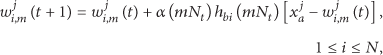
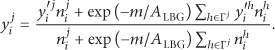
At the beginning of fusion part, each node sends its local results, $W_m^j=\{w_{i,m}^j;\hspace{0.17em}i=1,\dots ,N\}$ and $B_m^j=\{n_{i,m}^j,\hspace{0.17em}i=1,\dots ,N\}$ , to its neighbors. We then use the SOM weight updating formula to fuse received messages by considering the weights from neighbors as input data. For weights from node $j^{\prime }$ , node j adjust its weights as follows. First we find the best-matching weight in the local results of node j for each weight from node $j^{\prime }$ , $w_{i^{\prime },m}^{j^{\prime }}$ and denote the best-matching weight as $w_{b,m}^j$ . Then, the fusion weights are updated as

$$\begin{array}{l}{w}_{i,m+1}^j\\ \hspace{0.5em}=w_{i,m}^j+\frac{\alpha \left(m{N}_t\right){\sum }_{j^{\prime }\in {\Gamma }^j}{\sum }_{i^{\prime }}{n}_{i^{\prime },m}^{j^{\prime }}{h}_{bi}\left(m{N}_t\right)\left(w_{i^{\prime },m}^{j^{\prime }}-w_{i,m}^j\right)}{n_{i,m}^j+\alpha \left(m{N}_t\right){\sum }_{j^{\prime }\in {\Gamma }^j}{\sum }_{i^{\prime }}{n}_{i^{\prime },m}^{j^{\prime }}{h}_{bi}\left(m{N}_t\right)},\end{array}$$

(15)

where $h_{bi}$ is the neighbor kernel centered on the best-matching weight:

$$\begin{array}{cc}& h_{bi}\left(m{N}_t\right)=\exp \left(-\frac{{\parallel w_{b,m}^j-w_{i,m}^j\parallel }^2}{2{\sigma }^2\left(m{N}_t\right)}\right).\end{array}$$

(16)

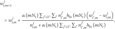
We here look back to the fusion updating formula of the distributed LBG algorithm. In fact, (8) can be rewritten as

$$\begin{array}{l}{y}_i^j=\frac{y_i^{\prime j}{n}_i^j+\exp \left(-m/A_{\text{LBG}}\right){\sum }_{h\in {\Gamma }^j}{y}_i^{\prime h}{n}_i^h}{n_i^j+\exp \left(-m/A_{\text{LBG}}\right){\sum }_{h\in {\Gamma }^j}{n}_i^h}\\ =y_i^{\prime j}+\frac{\exp \left(-m/A_{\text{LBG}}\right){\sum }_{h\in {\Gamma }^j}{n}_i^h\left(y_i^{\prime h}-y_i^{\prime j}\right)}{n_i^j+\exp \left(-m/A_{\text{LBG}}\right){\sum }_{h\in {\Gamma }^j}{n}_i^h}.\end{array}$$

(17)

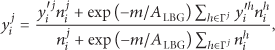
Obviously, (17) shows that the fusion updating formula of the distributed LBG algorithm has similar form of the distributed SOM. The distributed LBG algorithm uses simplified neighbors kernel—one for best matching weight and zero elsewhere. Thus, the distributed LBG fusion formula is the simplified case of the distributed SOM fusion formula. In the two distributed algorithms, local results from other nodes are considered as one kind of inputs that represent the data structure of other nodes' data and the fusion is one kind of SOM learning. In fact, (15) can also be seen as an iterative algorithm for distributed average consensus [24] with attenuation. Each node updates its own parameter by adding a weighted and attenuated sum of the total difference between its neighbors' parameters and its own. We use these updating rules to fuse the local results of different nodes to obtain the global reproduction vectors.

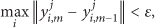
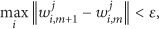
The terminal condition of distributed SOM is the same as distributed LBG. After updating, we compare the difference between $W_{m+1}^j$ and $W_m^j$ for node j with the threshold ϵ. If

$$\begin{array}{cc}& \underset{i}{\max }\parallel w_{i,m+1}^j-w_{i,m}^j\parallel <\epsilon ,\end{array}$$

(18)

node j enters terminated state. Terminated nodes do no computation or communication in following loops. If one node cannot receive messages from a neighbor in outer loops, the node will use the last messages from that neighbor when updating reproduction vectors. Otherwise, node j goes on to iteration $m+1$ of outer loop. When there is no message communication in the network, implying that all nodes have reached terminated state, the algorithm ends. After the algorithm ends, the final solution is obtained by computing the average of local weights. A summary of distributed SOM algorithm is given as follows.

Initialization. Local data $X^j$ for node j, initial weights $W_0^j=\{w_{i,0}^j;\hspace{0.17em}i=1,\dots ,N\}$    (the same for all nodes), inner loop parameter $N_t$ , and termination threshold ε.

Computation. Node j in iteration m of outer loop does

• (1)

Set $t\leftarrow 0$ and start inner loops. For each step of inner loops, rearrange input vectors in random order and then update the weights for each input vector

$$\begin{array}{cc}& w_{i,m}^j\left(t+1\right)=w_{i,m}^j\left(t\right)+\alpha \left(m{N}_t\right)h_{bi}\left(m{N}_t\right)\left[x_a^j-w_{i,m}^j\left(t\right)\right].\end{array}$$

(19)

 

Record the best-matching counts $B_m^j$ when doing adjusting. Set $t\leftarrow t+1$ after updating for one input vector and move on to the next. This inner loop is executed for $N_t$ times and self-organizing part ends when $t=N_t*L_j$ .

(2)

Send local results of node j, $W_m^j$ and $B_m^j$ , to its neighbors if node j is not terminated.

(3)

Find the best-matching weight for each received weight and update the fusion weights

$$\begin{array}{l}{w}_{i,m+1}^j\\ \hspace{0.5em}=w_{i,m}^j+\frac{\alpha \left(m{N}_t\right){\sum }_{j^{\prime }\in {\Gamma }^j}{\sum }_{i^{\prime }}{n}_{i^{\prime },m}^{j^{\prime }}{h}_{bi}\left(m{N}_t\right)\left(w_{i^{\prime },m}^{j^{\prime }}-w_{i,m}^j\right)}{n_{i,m}^j+\alpha \left(m{N}_t\right){\sum }_{j^{\prime }\in {\Gamma }^j}{\sum }_{i^{\prime }}{n}_{i^{\prime },m}^{j^{\prime }}{h}_{bi}\left(m{N}_t\right)}.\end{array}$$

(20)

 

If ${\max }_i\parallel w_{i,m+1}^j-w_{i,m}^j\parallel <\epsilon$ , the node enters terminated state. Otherwise, go to iteration $m+1$ of outer loop.

Termination. Algorithm ends when all nodes enter terminated state. The final weights are obtained by computing the average of local weights.

4.3. Communication Complexity Analysis

In this section, we estimate the communication complexity of the distributed SOM algorithm. Like what we do in the analysis of distributed LBG algorithm, let q denote $\text{ma}{\text{x}}_i\{{\Gamma }^i\}$ and I denote the total outer loops executed by the network before all nodes enter terminated state. Then, the number of total data messages transmitted by one node is $O(qIN)$ . Therefore, the number of total messages over J nodes is $O(JqIN)$ . Compared with the traditional SOM which needs all data available in one node and needs to transmit $O(JHL)$ vectors over the network, our distributed SOM algorithm requires less communication resource if there are large amounts of data distributed over the sensor network. We will give the simulation results in Section 5.4.4.

4.4. Computation Complexity Analysis

In this section, we present the computation complexity analysis of traditional SOM and distributed SOM. For each input vector in traditional SOM, we find the best matching weight in N weights and update all the N weights. Therefore, the computation complexity for one input vector is $O(N)$ and the total computation complexity is $O(Nt)$ where t is usually set as several times of $JL$ . For one node in distributed SOM, the computation complexity of inner loop is $O(N)$ for one input vector and $O(N_{t}NL)$ in total. From (15), the computation complexity for one fusing weight is $O(qN)$ . Therefore, the computation complexity of information diffusion is $O(q{N}^2)$ and is always insignificant in sensor network. Then, the total communication complexity for one node in distributed LBG is $O(N_{t}NLI)$ . The exact computation complexity is related to the network setup and algorithm parameters, and we will give the simulation results in Section 5.4.5.

5. Numerical Experiments

We study the behavior of distributed LBG algorithm and distributed SOM algorithm by simulation in this section. We first test our distributed algorithms under simple situation to observe the illustrative results. Then, tests of our algorithms under more complicated situation are also done to evaluate the performance in detail. In the following simulations, centralized LBG and centralized SOM, that is, traditional LBG and traditional SOM with input data gathered in one central processor, are denoted by c-LBG and c-SOM for short. Besides, nc-LBG and nc-SOM denote traditional algorithms carried out by each node with no-cooperation among nodes. Distributed LBG and distributed SOM are denoted by d-LBG and d-SOM.

In the simple situation, there are 10 nodes in the network and the input data are 2-dimensional, forming double-moon as showed in Figure 2. Each node has half inputs on one moon and half on the other. In other words, the inputs are balanced. Results of two different level quantizers, 8-level and 24-level, of the two distributed quantization algorithms are presented. Both of our distributed algorithms can obtain proper results under low and high level quantizer.

Figure 2

The illustrative results of our distributed algorithms. (a) Results of distributed LBG algorithm under low level quantizer. (b) Results of distributed LBG algorithm under high level quantizer. (c) Results of distributed SOM algorithm under low level quantizer. (d) Results of distributed SOM algorithm under high level quantizer.

In the complicated situation, much more detailed evaluation on the performance is presented. Here we first describe the simulation environment and the data generation. Then, we give the measure of performance of our vector quantization algorithms. At last, we present the results of our experiments.

5.1. Experiment Environment Setup

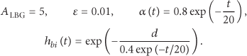
We test our distributed algorithms in networks consisting of 20 nodes. Nodes form a circle and each node is connected to two nearest nodes, respectively, in the left and right. Besides, two nonadjacent nodes are connected with a probability $P=0.1$ . The network topology is fixed during each trial. Each node is considered as a sensor and we concern the distributed quantization results over the sensor network. Besides, the parameters are set as

$$\begin{array}{cc}& A_{\text{LBG}}=5,\hspace{1em}\hspace{1em}\epsilon =0.01,\hspace{1em}\hspace{1em}\alpha \left(t\right)=0.8\exp \left(-\frac{t}{20}\right),\\ h_{bi}\left(t\right)=\exp \left(-\frac{d}{0.4\exp \left(-t/20\right)}\right).\end{array}$$

(21)

5.2. Data Generation

All the data used in our experiment are 2-dimensional data generated from a mixture of a square and two half-rings disturbed by uniform noise distributed over range $[-r/2,r/2]\times [-r/2,r/2]$ . The schematic plot of our experiment data is presented in Figure 3. The square and two half-rings are fixed during the experiment and the performances of our distributed quantization algorithms under different r values are tested.

Figure 3

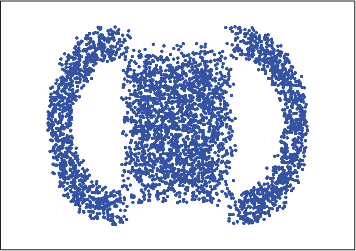
The schematic plot of experimental data.

To mimic the real sensor network environment, we test our algorithms using unbalanced data. Considering the center of the square as the origin of the coordinates, we divide the coordinate plane into four quadrants, $x>0$   &   $y>0$ ;   $x>0$   &   $y<0$ ;   $x<0$   &   $y<0$ , and $x<0$   &   $y>0$ . For each node, input vectors are chosen from the four quadrants. We describe the unbalance of the inputs in 5 levels. In level-0, inputs from all quadrants are balanced, chosen by the same probability, 25%. In level-1, inputs from a randomly selected quadrant are 40% and inputs from each of the other 3 quadrants are 20%, respectively. In level-2, the probabilities are 55% and 15%. In level-3, the probabilities are 70% and 10%. Finally, in level-4, the probabilities are 85% and 5%. Thus, the unbalanced inputs of one node can hardly reflect the overall data structure of all the data in network. The quantization results of each node using traditional quantization algorithms are far away from the other nodes' results. Each node has 200 input vectors in our experiments and the performances under different unbalance levels are tested to show the effect of unbalance.

5.3. Measure of Performance

We measure the performance of the quantization algorithms by the total distortion between each input vector and its corresponding reproduction vector. In this paper, we use the most common squared-error distortion for convenience. In addition to the results of our distributed LBG algorithm and distributed SOM algorithm, we also present the results of centralized LBG algorithm and centralized SOM algorithm, as well as the no-cooperation LBG algorithm and no-cooperation SOM algorithm. Obviously, centralized algorithms should perform best as the overall structure of data can be got at the cost of high communication complexity. We should be happy if the results of our distributed algorithms can approach that of the centralized algorithms, as we do not transmit the original input data. The no-cooperation distortion of a node is defined as the total distortion between all the input vectors and the individual quantization reproduction vectors of this node. Then, the overall no-cooperation distortion is the average of the distortion of all nodes.

In the numerical experiment, all the results are the average of independent 100 trails.

5.4. Result

To see the convergence process of the distributed algorithms, we present the distortion curves during outer loops of one typical trial in the balance case in Figure 4. As evident from the figure, the distortions of both distributed quantization algorithms decrease when algorithms carry on. Both algorithms converge after several outer loops. The distortion of distributed LBG is larger than that of distributed SOM. Moreover, the number of loops of distributed LBG is also larger than that of distributed SOM. What calls for attention is that the distortion curves during outer loops are just observed results. Whether the algorithms end or not depends on the max difference between the reproduction vectors of two sequential iterations of outer loop.

Figure 4

The evolution of the distortion of the distributed algorithms during outer loops.

5.4.1. The Influence of Unbalance

Here we present the performance of our distributed algorithms under different data unbalance conditions. Figure 5 shows the quantization distortion of distributed LBG algorithm ( $p=3$ ) and distributed SOM algorithm ( $N_t=20$ ), as well as the c-LBG, c-SOM, nc-LBG, and nc-SOM algorithms. The X-coordinate indicates the level of unbalance as stated in Section 5.2. The Y-coordinate indicates the total distortion. Figure 5(a) shows the results when $r=0.4$ and Figure 5(b) shows the results when $r=0.7$ .

Figure 5

Results of total distortion of quantization algorithms under different unbalance level. (a) The results when $r=0.4$ . (b) The results when $r=0.7$ . The distortions of no-cooperation algorithms in unbalance level-4 are too high so that they are not shown.

As evident from the figure, the results of distributed LBG algorithm are quite stable under different unbalance levels. The increase in unbalance does not have an obvious effect on the distortion performance. However, for the distributed SOM algorithm, the increase in unbalance has significant effect on the distortion performance. The performance of the distributed SOM algorithm is better than that of the distributed LBG algorithm under low unbalanced condition but worse under high unbalanced condition. The performance of distributed SOM under unbalance level-0 is particularly good and quite close to that of centralized SOM algorithm. The results of no-cooperation LBG and SOM are heavily worse than those of the distributed algorithms, especially under high unbalance level. The results under different r values lead to the same conclusion.

As analyzed in Sections 3.3 and 4.3, the communication complexity of our distributed algorithms is directly related to the number of outer loops executed by the algorithms. Figure 6 shows the number of outer loops needed by our distributed algorithms under different unbalance levels. Higher unbalance increases the number of outer loops needed by the distributed LBG obviously but nearly has no influence on the distributed SOM. The numbers of outer loops of the distributed LBG are significantly larger than those of the distributed SOM under all unbalance level conditions. Different r values have little influence on the number of outer loops for both the distributed LBG and SOM algorithms.

Figure 6

The number of outer loops of quantization algorithms under different unbalanced conditions.

5.4.2. The Influence of Inner Loop Parameter p

In the distributed LBG algorithm, p inner loops of traditional LBG-steps are executed in each node before information communication. We are interested in the influence of inner loop parameter p. We check the distortion performance and outer loops of our distributed LBG algorithm with different parameter p under different unbalance levels. Figure 7 shows the distortion performances of $p=1$ , $p=3$ , and $p=5$ .

Figure 7

The total distortion of distributed LBG algorithm under different p values.

In both $r=0.4$ and $r=0.7$ , the distortion performances of $p=1$ are obviously worse than those of larger p values. The experiment results show that a few more inner loops improve the distortion performance. The curves of $p=3$ and $p=5$ are close to each other for both $r=0.4$ and $r=0.7$ . We do not show the curves of $p=2$ and $p=4$ here because they are both lower than the curve of $p=1$ and nearly coincide with the curves of $p=3$ and $p=5$ . The increase in r directly results in the increase in distortion but the distortion curves change little under different unbalance levels.

Figure 8 shows the outer loops needed by distributed LBG algorithms under different p values. The loops needed when $p=1$ are obviously greater than those needed when $p>1$ . But the results are close to each other when $p>3$ . More inner loops done by each node lead to less outer loops. The conclusions are similar under different r values, so we only show the results when $r=0.4$ . We suggest setting $p=3$ as we have done in Section 5.4.1 to get a better distortion performance, meanwhile, reduce communication complexity.

Figure 8

The number of outer loops needed by distributed LBG algorithm under different p values.

5.4.3. The Influence of Inner Loop Parameter $N_t$

In the distributed SOM algorithm, $N_t$ is the inner loop parameter indicating the steps of inner loops done before message transmission. We are interested in the influence of parameter $N_t$ . We check the distortion performance and the number of outer loops of the distributed SOM algorithm with different $N_t$ under different unbalance levels. Figure 9 shows the distortion performances of $N_t=1,5,10,20$ when $r=0.7$ .

Figure 9

The total distsortion of distributed SOM algorithm under different $N_t$ when $r=0.7$ .

From Figure 9, we can see that the distortion curve of $N_t=1$ is the lowest of the 4 curves showed in the picture. The distortion curves of $N_t=5$ , $N_t=10$ , and $N_t=20$ are higher than those of $N_t=1$ and close to each other. More steps in inner loop result in the increase of distortion. The similar results can be found when $r=0.4$ .

Figure 10 shows the outer loops needed by distributed SOM algorithm when $r=0.7$ . Larger $N_t$ leads to smaller number of outer loops needed. The number of outer loops needed when $N_t=1$ are significantly greater than the rest and nearly 15 times of that when $N_t=20$ . The number of outer loops needed under different unbalance level almost remains unchanged for larger inner loop parameter. We here notice that the products of inner loop parameter $N_t$ and the corresponding number of outer loops are quite similar (about 80–100) for different $N_t$ . This means that the total computing time is almost the same for different $N_t$ while less communication is needed for larger $N_t$ condition, since the number of outer loops is exactly the times of messages exchange. The results when $r=0.4$ are similar. In consideration of the results showed in Figure 9, we suggest setting $N_t=20$ as we have done in Section 5.4.1 to get a balance between distortion and communication complexity.

Figure 10

The number of outer loops needed by distributed SOM algorithm under different $N_t$ values.

5.4.4. The Communication Complexity Performance

Here we present the communication complexity performance of our distributed algorithms. We check the performance of $L=200,\mathrm{\hspace{0.17em}\hspace{0.17em}}500,\mathrm{\hspace{0.17em}\hspace{0.17em}}1000,\mathrm{\hspace{0.17em}\hspace{0.17em}}2000$ with $p=3$ , $N_t=20$ . From Figure 11, we see that the communication complexity increases with the increase of L. The communication needed by traditional algorithms increases linearly because the communication complexity is directly related to the number of input vectors. On the other hand, the communication needed by distributed algorithms changes little because the communication complexity has nothing to do with the number of input vectors. The communication of distributed algorithms is related to the number of outer loops, and the increase of input vectors has little influence on the outer loops. Therefore, for large amount of input vectors, our distributed algorithms show superiority on communication complexity performance. For our distributed algorithms, we see that the distributed LBG needs more communication than the distributed SOM.

Figure 11

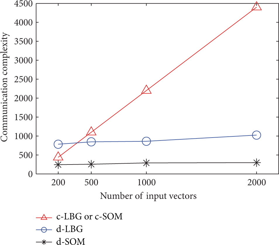
The communication complexity performance of distributed and traditional algorithms under different numbers of input vectors of each node.

5.4.5. The Computation Speed Performance

Here we present the computation speed performance of our distributed algorithms. The simulation is run by matlab 7.0 and using a PC with CPU of 2.1 GHz and 2 G RAM. We check the computing time (seconds) of different L, $L=200,\mathrm{\hspace{0.17em}\hspace{0.17em}}500,\mathrm{\hspace{0.17em}\hspace{0.17em}}1000,\mathrm{\hspace{0.17em}\hspace{0.17em}}2000$ with $p=3$ , $N_t=20$ . As the actual running time of distributed algorithms in sensor network is decided by the node which needs the longest time, we compare the computing time of one node in distributed algorithms with the time needed by traditional algorithms. From Figure 12, we see that the computing time of both the traditional and distributed algorithms increases when the number of input vectors increases. But the computing time of the distributed algorithms is less than that of the traditional algorithms because in actual sensor network, the distributed algorithms distribute the computation to each node and nodes can realize the vector quantization parallelly. Therefore, compared with the traditional algorithms, our distributed algorithms can improve the computation speed. From the picture, we can also see that distributed SOM needs more computation time than the distributed LBG.

Figure 12

The computation time of the distributed and traditional algorithms under different numbers of input vectors of each node. (a) The results of the distributed LBG and traditional LBG. (b) The results of the distributed SOM and traditional SOM.

6. Conclusion

In this paper, we consider vector quantization in the situation that data are distributed over network. Traditional vector quantization algorithms are not feasible for distributed data because they need all the data available in a central processor which results in heavy data communication burden. Thus, in this paper, we propose two distributed quantization algorithms to solve the distributed quantization problem without centralizing the data to one node. Our distributed algorithms work by local quantization and neighbor communication. Our experiments show that the distributed LBG algorithm has a stable distortion performance under different unbalance levels but costs more outer loops than the distributed SOM algorithm. The distortions of the distributed LBG are little affected by data of different unbalanced degree, while the outer loops needed increase obviously when the degree of unbalance increases. The distortion performances of the distributed SOM are significantly affected by the unbalance level and get larger obviously when unbalance level increase. The outer loops of distributed SOM are less than that of the distributed LBG and almost stay unchanged when the unbalance level increases. As a conclusion, the distributed LBG algorithm is more suitable for unbalanced condition while the distributed SOM algorithm is more suitable for balanced condition. Compared with the centralized algorithms which need all data available in one node, our distributed algorithms require less communication resource if there are large amount of data distributed over the sensor network. When the communication resource is severely limited, the distributed SOM algorithm is more preferred, since the number of outer loops (the times of communication) needed is small.

As our algorithms are based on basic vector quantization algorithms, we believe that some other centralized vector quantization algorithms can also be extended to distributed version using our distributed protocol. For example, we may develop distributed vector quantization based on information theory.