Sage Journals: Discover world-class research

Abstract

This paper presents the mathematical model of screw compressors’ working process, in which the internal flow domains are divided into three kinds of fluids—the inlet fluid, the primitive volume fluid, and outlet fluid. Grid interface method and dynamic mesh technique of Computational Fluid Dynamics (CFD) theory were utilized to simulate the suction, compression, and discharge process in order to model the dynamic characteristics of the flow domains in a screw compressor. To verify that the model is numerically accurate and the simulation method is effective, experiments on the pressure-volume changes in screw compressor were carried out. The result has shown that the simulation data is in good agreement with the experimental data. Therefore, the numerical calculation model and the simulation method can be very useful for the screw compressor design and research.

1. Introduction

Screw compressors play a significant role in the rotary compressor and have been widely used in various industrial fields with the advantages of its compact structure, smooth operation, high efficiency, small size, and so forth. To further analyze the performance of screw compressors, a lot of investigations have been done by domestic and foreign scholars for both oil-free and oil-injected compressors: Wu et al. [1, 2] put forward a novel mathematical model of screw compressors and verified its rationality by experimental tests; Kovacevic et al. [3, 4] applied a numerical method to the screw machine and proposed that the method is widely applicable to the fluid mechanical study; Cao et al. [5] researched on the screw compressor inner pressure distribution by experiments and later became specialized in the pressure distribution of the inlet and outlet port; Zhang et al. [6] studied the screw compressor discharge pressure pulsation by experiment and found the discharge pressure pulsation is caused by the actual values deviate from the design. All these people did a lot of research and analysis through theoretical calculations and practical experiments on the internal flow domains and the performance of screw compressors. While the theoretical calculations are proven to evaluate and predict the performance of screw compressors whose design parameters are known in advance, it is less accurate than the estimate from the results of experiments. Experimental analysis can directly reflect the performance of a screw compressor. However, in order to carry out the experiments, purposely designed helical rotors and casing have to be made. That often leads to long design cycle and high associated cost and makes the entire development of the compressor expensive.

The advent of digital computing made it possible to model the compression process more accurately. With the passage of time, ever more detailed models of the internal flow process have been developed, based on the assumption of one-dimensional nonsteady bulk fluid flow and one-dimensional steady leakage flow through the working chamber. This paper establishes a reasonable and effective screw compressor fluid model, in which the dynamic characteristics of the flow domains of the screw compressor were simulated through dynamic mesh and software Fluent. The paper also includes the experiment results to justify the correctness of dynamic simulation results. The paper concludes by claiming that the dynamic simulation method provides an effective means for improving the design of screw compressors.

2. Structure and Principle

As shown in Figure 1, a screw compressor consists of a pair of intermeshing helical rotors parallelly installed in the body. The rotor which has convex teeth on the outside of the pitch circle is called male rotor and the other one with concave teeth on the inside of the pitch circle is called the female rotor. Usually the male rotor is connected with the original motivation and drives the female rotor through the synchronous gears between them. Two orifices with defined shape and size are opened at both ends of the screw compressor body. The one for the getter is named the inlet port and the other one for the discharge is called the outlet port.

Figure 1:

Basic structure of the twin screw compressor.

The working process of a screw compressor is a cyclic process which can be divided into three subprocesses: air suction, compression, and discharge. As the rotors rotate, each pair of intermeshing teeth is completing the same working cycle. When the rotors turn a certain angle, the male rotor convex teeth invade the female rotor concave teeth, meanwhile, the isolated primitive volume between the teeth begin to shrink to realize gas compression until it connects with the outlet port. After that the discharge process starts and continues until the two teeth are fully engaged. At that point, the primitive volume falls to zero.

3. Dynamic Simulation Analysis

The following assumptions are made to establish the dynamic numerical model of the working process.

The compressed gas is assumed to be ideal.

The working medium does not leak to the outside environment.

Lubricating oil has no effect on the nature of the working medium.

The gas flow through the inlet port and outlet port is isotropic.

The screw compressor working cycle is a theoretical cycle.

Screw compressor fluid dynamic analysis process based on CFD is shown in Figure 2.

Figure 2:

Working process of CFD analysis.

3.1. Numerical Calculation Model

Modeling the working process of a screw compressor is complex. To mimic each working cycle of air suction, compression, and discharge, the model must consider the on-and-off connection of a primitive volume and the inlet port or the outlet port. Therefore, the screw compressor fluid model is divided into three parts—inlet port fluid, primitive volume fluid, and outlet port fluid. All three fluids are controlled through the grid interface settings. When establishing the primitive volume fluid in particular, we set the gap between the male and female rotors and the wall to 0.3 mm, and the center distance between the rotors by 0.3 mm in accordance with the requirement that the moving grid needs to leave a certain gap between the moving parts. The calculation domain model in this paper is shown in Figure 3.

Figure 3:

The flow domains of screw compressor.

3.2. Establishment of the Control Equation

The internal fluid of screw compressor is highly complex. It is three-dimensional unstable irregular fluid flow with rotation, which is a typical turbulence model [7, 8]. The modified RNG/k − ∊ model can be good at simulating the fluid due to its strong bend flow line, swirls, and rotating flow. Using compressed and modified RNG/k − ∊ model instead of the traditional model to simulate the internal flow of screw compressor cavity avoids distortion and stays closer to the actual situation. As in this paper, the RNG/k − ∊ model is applied to simulate the fluid flow in screw compressors.

Large-scale movement and modified viscosity item help to reflect the influence of small-scale movements in the RNG/k − ∊ model. By systematically removing these small-scale movements from the control equation, we obtained the turbulence kinetic energy equation (k equation) and the turbulent dissipation rate equation (∊ equation).

The turbulence kinetic energy equation (k equation) can be expressed as the following:

\frac{\partial}{\partial t} (ρ k) + \frac{\partial}{\partial x_{j}} (ρ μ_{j} k - \frac{u_{e f f}}{δ_{k}} \frac{\partial k}{\partial x_{j}}) = μ_{i} (P + P_{B}) - ρ ε - \frac{2}{3} (μ_{i} \frac{\partial μ_{i}}{\partial x_{i}} + ρ k) \frac{\partial μ_{i}}{\partial x_{i}} .

(1)

The turbulent dissipation rate equation (∊ equation) is described as below:

\frac{\partial}{\partial t} (ρ ε) + \frac{\partial}{\partial x_{j}} (ρ μ_{j} ε - \frac{u_{e f f}}{δ_{k}} \frac{\partial ε}{\partial x_{j}}) = C_{ε 1} [\frac{ε}{k} μ_{i} P - \frac{2}{3} (μ_{i} \frac{\partial μ_{i}}{\partial x_{i}} + ρ k) \frac{\partial μ_{i}}{\partial x_{i}}] - C_{ε 2} ρ \frac{ε^{2}}{k} + C_{ε 3} ρ \frac{ε}{k} μ_{i} P_{B} + C_{ε 4} ρ ε \frac{\partial μ_{i}}{\partial x_{i}} - \frac{C_{μ} η^{3} (1 - η / η_{0})}{1 + β η^{3}} \frac{ρ ε^{3}}{k},

(2)

μ_{f f} = μ_{t} + μ,

(3)

where μ is the dynamic viscosity coefficient; μ_t is the turbulent viscosity coefficient, defined as C_μρk²/∊; C_μ is a constant; δ_∊ is the turbulent Prandtl number of turbulence kinetic energy dissipation rate ∊; δ_k is the turbulent Prandtl number of turbulence kinetic energy k; s_ij is the tensor of fluid deformation rate; P_B = − (g_i/ρ) (∂ρ/∂x_i); g_i is the gravitational acceleration at direction i; η = S(k/∊), S = (2s_ijs_il)^1/2. C_μ, δ_k, δ_∊, C_∊1, C_∊2, C_∊3, C_∊4, η₀, β, and other empirical coefficients in the formula (2) are shown in Table 1.

Table 1:

RNG/k − ∊ turbulence model coefficient.

C _μ	δ_k	δ_∊	C _∊1	C _∊2

0.08	0.71	0.719	1.41	1.68

C _∊3	C _∊4	η₀	β

1.42	−0.387	4.38	0.012

3.3. Determination of Boundary Conditions and Initial Conditions

To dynamically simulate the distribution of the internal flow in a screw compressor, we used the Fluent software. The first step was to determine the model boundary conditions [9] and configure their related settings. This can be key to the screw compressor fluid model and dictate whether the simulation of air suction, compression, and discharge process is in line with the actual working situation.

Fluid boundary condition types are shown in Table 2.

Table 2:

Fluid boundary type.

Boundary name	Boundary type	Boundary name	Boundary type

Inlet port	Pressure inlet	Interface 2-1	Interface
Outlet port	Pressure outlet	Interface 2-2	Interface
Left rotating wall	Wall	Interface 3-1	Interface
Right rotating wall	Wall	Interface 3-2-1	Interface
Interface 1-1	Interface	Interface 3-2-2	Interface
Interface 1-2	Interface	Other walls	Wall

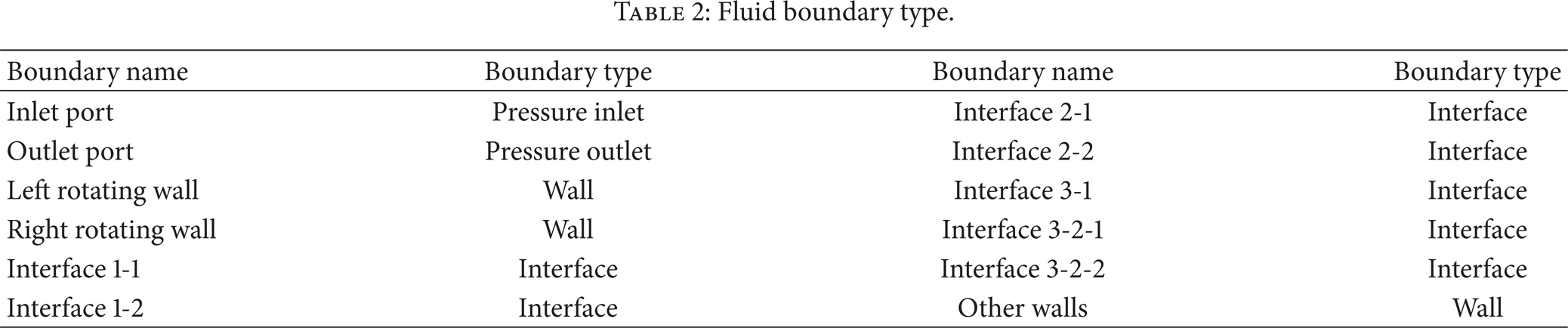
Pairing the interface 1-1 with 1-2, 2-1 with 2-2, 3-1 with 3-2-1 and 3-2-2, we guaranteed that the overlapped boundary in the pairing interfaces is an interior boundary. Therefore, we ensured that the fluid is interconnected from entrance to exit through the grid interface settings in Fluent software.

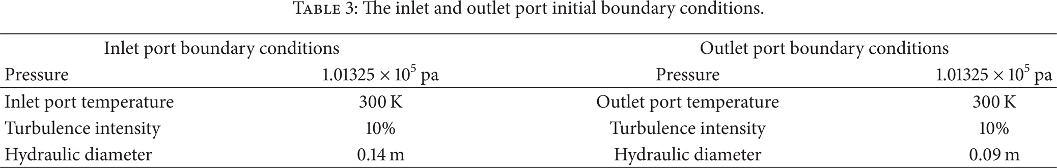
The settings of the inlet and outlet port of the initial boundary conditions are shown in Table 3.

Table 3:

The inlet and outlet port initial boundary conditions.

Inlet port boundary conditions		Outlet port boundary conditions
Pressure	1.01325 × 10⁵ pa	Pressure	1.01325 × 10⁵ pa

Inlet port temperature	300 K	Outlet port temperature	300 K
Turbulence intensity	10%	Turbulence intensity	10%
Hydraulic diameter	0.14 m	Hydraulic diameter	0.09 m

3.4. Dynamic Mesh Technique

The original grid of the screw compressor fluid model was generated in the Gambit software in which the mesh of three-dimensional fluid model can be mapped with tetrahedron and hexahedron grids. A common problem of dynamic mesh [10, 11] when used to simulate and analyze the model is that, after smoothing and remeshing, mesh distortion of some parts is very serious. Since unstructured tetrahedral grid adapts the distortion better, it is used to mesh the primitive volume fluid. The model is therefore divided into 2,317,448 tetrahedral grid cells. The grids of inlet and outlet fluid are stationary and therefore can be both structured and unstructured. However, in order to be consistent with the grid type of primitive volume fluid, the grids of the inlet and outlet fluid model are chosen to be unstructured. The fluid model at the inlet port is divided into 470,861 tetrahedral grid cells while the fluid model at the outlet port is divided into 171,296 tetrahedral grid cells. The mesh of the fluid model is shown in Figure 4.

Figure 4:

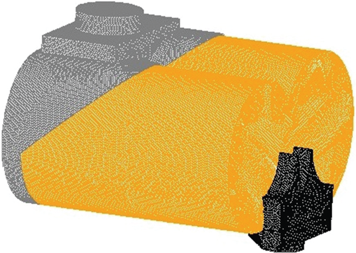
Mesh of the model.

The grid is updated automatically by Fluent triggered by the change of boundary in each iteration. The two rotors in the screw compressor follow the uniform circular motion, which has a large displacement. To simulate this motion, we combined the spring smoothing approximation model with the partial remeshing model to update the grid. When the rotation angle between male and female rotors is very small, every edge of the grid around the rotors can be seen as a spring, which has a tiny deformation when the rotors rotate. When the rotation angle becomes large, the grid begins remeshing locally to meet the requirement of the grid cell size when the mesh deformation around the rotors exceeds a certain limit.

Dynamic mesh calculation is dependent on the movement pattern [12] of the dynamic mesh zone. If the dynamic mesh zone follows a rigid body motion, both the profile function and the UDF can be used to model the movement. If the dynamic mesh zone is a deformation area, only UDF can be used to define the geometric characteristic feature and partial remeshing parameters. Therefore, if the dynamic grid area experiences both rigid body motion and deformation, UDF should be used to model the geometric change and movement. In this paper, the movement of male and female rotors is defined through the profile function because their rotation does not involve deformation and can be regarded as a rigid body motion in the dynamic simulation of the screw compressor.

The profile function of female rotor:

((rotating_left 3 point)

(time 0 1 60)

(omega z −309.813 −309.813 −309.813))

The profile function of male rotor:

((rotating_right 3 point)

(time 0 1 60)

(omega z 258.1775 258.1775 258.1775))

3.5. The Simulation Results and Analysis

The basic parameters of the screw compressor for the simulation in this paper are shown in Table 4.

Table 4:

Screw compressor basic parameters.

Parameters
Male rotor outer diameter	359.470 mm
Female rotor outer diameter	319.341 mm
Male rotor wraps angle	300.634°
Theoretical volume displacement	13.001 m³/min
Normal pressure	0.7 Mpa
Velocity of rotation	2940 rpm

The simulation results are shown in Figures 5 –9.

Figure 5:

Pressure distribution of flow domains.

Figure 6:

Velocity vectors distribution of flow domains.

Figure 7:

Density distribution of flow domains.

Figure 8:

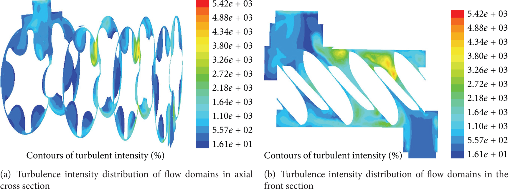
Turbulence intensity distribution.

Figure 9:

The flow pathlines based on pressure distribution of the flow domains.

Figure 5 is the screw compressor flow model pressure distribution cloud, wherein Figure 5(a) shows the pressure contours at the cross section in the axial direction, and Figure 5(b) shows pressure contours at the male and female rotors meshing zone in the front section. The red area in the figure indicates high pressure while the blue area indicates low pressure (the same below). Figure 5 shows that the maximum pressure of the entire flow domains is 0.740 Mpa, occurring in the outlet port, and the minimum pressure is −0.0628 Mpa, occurring at the inlet, the female, and the male rotor meshing zone. In particular, Figure 5(a) shows that pressure rises as the flow domains move from the inlet to the outlet port. Figure 5(b) shows that, with the plane through the male and female rotor axes dividing the flow domain, the pressure of the upper part connected to the inlet port is lower than the pressure of the lower part connected to the outlet port.

Figure 6 is the screw compressor flow model velocity vectors distribution cloud, wherein Figure 6(a) shows the velocity vectors at the cross section in the axial direction, and Figure 6(b) shows velocity vectors at the male and female rotors meshing zone in the front section. As seen from Figure 6, the velocity of the entire flow domain stays relatively stable, with the flow speed at the inlet port, the outlet port, and the convergence of wall and the male and female rotors meshing relatively larger than the rest. The inlet gas in the negative pressure state is rapidly sucked into the compression chamber, which leads to high velocity while the velocity of the fluid at the corner location of the inlet and outlet stays low; the instantaneous speed of the fluid at the outlet port connected to the pressure vessel and gas reflux is high at the instant of the outlet port being connected; the gas fleeing from the high pressure area to the low pressure area carries great velocity, which is caused by the gaps between the wall and the female and male rotors meshing.

Figure 7 is the screw compressor flow model density distribution cloud, wherein Figure 7(a) shows the density contours at the cross section in the axial direction, and Figure 7(b) shows the density contours at the male and female rotors meshing zone in the front section. The pressure is proportional to the density so the density distribution and the pressure distribution are roughly the same—the density of the low pressure area is small and the density of the high pressure area is large.

Figure 8 is the screw compressor flow model turbulence intensity cloud, wherein Figure 8(a) shows the turbulence intensity contours at the flow cross section in the axial direction, and Figure 8(b) shows the turbulence intensity of the flow at the male and female rotors meshing zone in the front section. As seen from Figure 8, the high-speed rotation of rotors drives fluid to converge together from different directions to form a strong vortex in the vicinity of the male and female rotors meshing so the nearby turbulence intensity is large. The flow fluid is relatively regular at the location of the inlet and outlet so the turbulence intensity there is small.

Figure 9 is the flow pathlines based on the pressure distribution of the screw compressor flow domains. It can be seen from Figure 9 that the gas follows vortex motion in each primitive volume from the inlet port to the outlet port, meets at the place of the male and female rotors meshing with the rotors ration, and finally gets compressed toward the outlet port. That completes the entire working cycle from suction to compression and to discharge.

4. Experimental Research and Analysis

In this paper, the screw compressor with the same parameters of those input into the fluid dynamics simulation model was studied by experiments to verify the CFD theory is suitable for the dynamic simulation of screw compressor working process. We assumed the change of pressure of every primitive volume of screw compressor in a working cycle is the same. Since each of the primitive volumes is closed at the end of the suction and the volume decreases until the gas is discharged through the outlet, a small pressure sensor with high sensitivity was embedded in the bottom of female rotor at the discharge side to measure the change of pressure inside groove from midpoint suction stroke to the completion of discharge.

The position of the pressure sensor embedded in the female rotor and in the data acquisition system is shown in Figures 10 and 11, respectively. The type of sensor is XTL-193-190 (M), the overall error of integrated nonlinearity, hysteresis, and repeatability value of the sensor is less than ±0.5% and its natural frequency is 700 Hz, its resolution is infinitesimal, the maximum working pressure is 3.5 Mpa, and the range of working temperature is from −55°C to 204°C. As shown in Figure 11, the leading wire of pressure sensor passes through the center hole of the female rotor and is connected to a slip-ring by coupling. Signals will be amplified by the signal amplifier and then it will be collected to the acquisition instrument, and finally will be processed and analyzed by data process system.

Figure 10:

The location of the pressure sensor.

Figure 11:

Test data acquisition and analysis system.

The pressure is extremely important since it is used to construct a P-V indicator diagram of the compressor. If the constructed P-V indicator diagram from the dynamic simulation is consistent with the measured one, that means the overall performance of the compressor is well predicted by the dynamic simulation. The P-V indicator diagrams of the dynamic simulation and the measured results under the full load are compared in Figure 12. As seen from the figure, the dynamic simulation results and the measured results coincide well, particularly in the compression process. In the early stage of the compression process, simulation results are off from the experimental results by a steady drop in pressure rather than decreased first and then on the rise. That is because the model for dynamic simulation has no structure of the slide valve which prevents the pressure in compression chamber from connecting with the suction chamber in the early compression stage and the pressure in compressor will increase. In the discharge process, the simulation model also accurately reflects the real discharge process of screw compressor. Overall, for the same screw compressor dynamic simulation data agrees well with the experimental data, which proves the correctness and effectiveness of the dynamic simulation method.

Figure 12:

P-V indicator diagram of measured results and simulation results.

5. Conclusions

(1) The study of the internal flow domains of a screw compressor has shown us that the pressure from the inlet to the outlet along the axial direction is increasing. We can further conclude that each primitive volume is the same and the pressure within the volume increases from the inlet to the outlet. The speed at the gap between the male and female rotors and the cavity wall is large, which shows that there is serious leakage in the gap. The turbulence intensity distribution and the flow pathlines reflect the complexity of the screw compressor internal fluid flow.

(2) Experiments were carried out to study the P-V indicator diagram of the screw compressor. By comparing diagrams of the dynamic simulation results and measured results, we observed that the two results coincide well, which proves that the numerical calculation model and dynamic simulation method in this paper are correct and effective.

(3) If an effective and reliable numerical model is established and reasonable initial conditions, boundary conditions, and parameter settings are set, CFD theory and technique can be effectively used for an accurate simulation. That again emphasizes that the numerical calculation model and the simulation method are very useful for the screw compressor design and research.

Conflict of Interests

The authors declare that there is no conflict of interests regarding the publication of this paper.

Footnotes

Acknowledgments

The financial support for this research is provided by National Nature Science Foundation of China under Grant no. 51275210 and no. 51105175, Six-Major-Talent-Summit Project of Jiangsu Province (2013-ZBZZ-016), and Industry-University-Research Foundation of Jiangsu Province (BY2013015-30). Their help is greatly appreciated.

References

Xing

, and Shu

, “Theortical and experimental study on indicator diagram of twin screw refrigeration comperssor,” International Journal of Refrigeration, vol. 27, no. 4, pp. 331–338, 2004.

, and Xing

, “Theoretical and experimental research on the working process of screw refrigeration compressor under superfeed condition,” International Journal of Refrigeration, vol. 30, no. 8, pp. 1329–1335, 2007.

Kovacevic

Stosic

Mujic

, “Advances in numerical modelling of helical screw machines,” in Proceedings of the International Compressor Engineering Conference, pp. 1158–1166, July 2010.

Kovacevic

Stosic

, and Smith

I. K.

, “A numerical study of fluid-solid interaction in screw compressors,” International Journal of Computer Applications in Technology, vol. 21, no. 4, pp. 148–158, 2004.

Cao

Gao

Xing

, and Shu

, “Experimental analysis of pressure distribution in a twin screw compressor for multiphase duties,” Experimental Thermal and Fluid Science, vol. 35, no. 1, pp. 219–225, 2011.

Zhang

Peng

, and Xing

, “Theoretical and experimental research on the discharge pressure pulsation of screw compressors,” Compressor Technology, vol. 6, pp. 3–6, 2001.

Hongfei

Hongsong

, and Handong

, “The choice of turbulence model in numerical simulation,” Journal of Projectiles, Rockets, Missiles and Guidance, vol. 4, pp. 242–244, 2006.

Lin

Zhixiang

Peng

, “Application study on the turbulence models of k-e. Quadratic equation on CFD calculation,” Ship Engineering, vol. 3, pp. 5–8, 2010.

Malcevic

and Ghattas

, “Dynamic-mesh finite element method for Lagrangian computational fluid dynamics,” Finite Elements in Analysis and Design, vol. 38, no. 10, pp. 965–982, 2002.

10.

Tang

, “Moving mesh methods for computational fluid dynamics,” in Recent Advances in Adaptive Computation , vol. 383 of Contemporary Mathematics, pp. 141–174, 2005.

11.

Klingner

B. M.

Feldman

B. E.

Chentanez

, “Fluid animation with dynamic meshes,” ACM Transactions on Graphics, vol. 25, no. 3, pp. 820–825, 2006.

12.

Ahn

H. T.

Branets

, and Carey

G. F.

, “Moving boundary simulations with dynamic mesh smoothing,” International Journal for Numerical Methods in Fluids, vol. 64, no. 8, pp. 887–907, 2010.