FPGA Implementation of Self-Organized Spiking Neural Network Controller for Mobile Robots

Abstract

Spiking neural network, a computational model which uses spikes to process the information, is good candidate for mobile robot controller. In this paper, we present a novel mechanism for controlling mobile robots based on self-organized spiking neural network (SOSNN) and introduce a method for FPGA implementation of this SOSNN. The spiking neuron we used is Izhikevich model. A key feature of this controller is that it can simulate the process of unconditioned reflex (avoid obstacles using infrared sensor signals) and conditioned reflex (make right choices in multiple T-maze) by spike timing-dependent plasticity (STDP) learning and dopamine-receptor modulation. Experimental results show that the proposed controller is effective and is easy to implement. The FPGA implementation method aims to build up a specific network using generic blocks designed in the MATLAB Simulink environment. The main characteristics of this original solution are: on-chip learning algorithm implementation, high reconfiguration capability, and operation under real time constraints. An extended analysis has been carried out on the hardware resources used to implement the whole SOSNN network, as well as each individual component block.

1. Introduction

A new computational formalism has recently emerged called spiking neural network (SNN). Unlike the traditional neural networks (e.g., the MP model), SNNs code information in the form of spike trains, just as biological neurons do. It has been proven that the spiking model can do everything that traditional models could, often with many fewer neurons [1]. SNNs can act as brain, controlling and navigating mobile robots. SNNs have at least two properties that make them interesting candidates for adaptive control of autonomous behavioral robots [2, 3]. First, the intrinsic dynamic information of SNNs is based on the precision of the spike firing times. This allows the temporal patterns of sensory-motor events to be captured and exploited more efficiently than networks with analog neurons. Second, it is possible to implement large networks of spiking neurons in tiny and low-power chips [4] because the spikes are in essence binary events and the nonlinear dynamics and the coding of spiking circuits can be provided by spiking times.

Due to these advantages SNN researchers have tried to employ SNNs in the robotic area. Floreano and colleagues [2, 3] proposed a SNN topology based on Genetic Algorithms (GA), and applied it to the Kephera robot controllers for wall following. The GA they used evolved signs (excitation/inhibition) and connections (present/absent) between neurons. Their work demonstrated that evolution can discover functional networks by searching the space of connectivity. In [5], Hagras et al. designed a mechanism to control autonomous mobile robots and to perform a wall following task, using a SNN (with Spike Response Model) in combination with online adaptive genetic algorithm to evolve weights and signs. The input layer was fed with values from the ultrasound sensors converted to spikes using a “delay coding” system. Alnajjar and Murase [6] continued working with the Kephera robot, based on Floreano's work. They successfully designed a self-organization algorithm of SNN for an autonomous robot. Letting it evolve by changing the sign and connections of the network synapses for the obstacle avoidance task and demonstrated that it accomplishes faster than using an online GA. In paper [7], Wang et al. developed a SNN controller similar to the one that Hagra and Pouds created. They trained the SNN using Hebbian learning instead of GA to make the robot capable of avoiding obstacles.

In this work, a SNN is used to control a robot based on encoded inputs from sensors obtaining information about robot's environment. The robot's goal is to pursue the brightest location in a multiple T-maze using light sensors, infrared sensors, and color sensors. In this control model the tunable parameters are the synaptic connection weights, which are evolved by spike-timing-dependent plasticity (STDP) and dopamine-receptor modulation. This work extends the STDP-SNN paradigm by linking the simulator to the robot hardware.

This paper is organized as follows. Section 2 introduces the basics of SOSNN and discusses the principle of the behavior controller in detail. Section 3 presents the hardware implementation. The paper is concluded in Section 4.

2. Spiking Neural Network with Reconfigurable Connectivity

2.1. Neuron Model

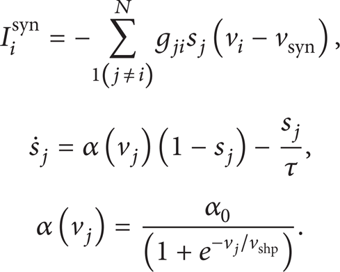
Various spiking neuron models exist, such as the leaky integrate-and-fire (I&F) neuron [8], Fitzhugh model [9], Izhikevich (IZH) model [10], and Hodgkin-Huxley (HH) model [11]. Among these models, the HH is the most biologically accurate model currently used, but it is highly complex. In the experiments described in this paper, we have chosen the IZH neuron model, which has been shown to be both biologically plausible and computationally efficient [12]. The membrane potential dynamics is described by

$\begin{array}{l}{\dot{v}}_i=\mathrm{0.04}{v}_i^{\mathrm{2}}+\mathrm{5}{v}_i+\mathrm{140}-u_i+I_{\text{input}}+I_i^{\text{syn}}\\ {\dot{u}}_i=a(b{v}_i-u_i)\end{array}$

(1)

$\text{if}\hspace{0.17em}\hspace{0.17em}{v}_i>\mathrm{30}\hspace{0.17em}\text{mV},\hspace{1em}\text{then}\{\begin{array}{cc}{v}_i⟵c\hfill & \hfill \\ u_i⟵u_i+d,\hfill & \hfill \end{array}$

(2)

where i = 1, 2, 3,…, N. N is the number of neurons. v _i represents the membrane potential of the neuron i and u _i is a membrane recovery variable. The parameter a describes the time scale of the recovery variable u _i . Smaller values result in lower recovery. The parameter b governs the degree of neuron's excitability. Neurons with larger b are prone to exhibit larger excitability and fire with a higher frequency than others. The parameter c describes the after-spike reset value of the membrane potential v _i caused by the fast high-threshold K⁺ conductances. The parameter d describes after-spike reset of the recovery variable u _i caused by slow high-threshold Na⁺ and K⁺ conductances. The model can exhibit firing patterns of all known types of cortical neurons with the choice of parameters a, b, c, and d given in [10]. In this paper, in order to establish a heterogeneous network, the initial values of b _i are randomly distributed in (0.12, 0.2). Others are set to be typical values for regular spiking type: a = 0.02, c = − 65, and d = 2 [10]. I_input stands for the externally applied current and I _i ^syn is the total synaptic current through neuron i and is governed by the dynamics of the synaptic variable s _j [13]:

$\begin{array}{c}{I}_i^{\text{syn}}=-{\displaystyle \sum }_{\mathrm{1}\left(j\ne i\right)}^N{g}_{ji}{s}_j\left(v_i-v_{\text{syn}}\right),\\ {\dot{s}}_j=\alpha \left(v_j\right)\left(\mathrm{1}-s_j\right)-\frac{s_j}{\tau },\\ \alpha \left(v_j\right)=\frac{{\alpha }_{\mathrm{0}}}{\left(\mathrm{1}+e^{-v_j/v_{\text{shp}}}\right)}.\end{array}$

(3)

Here the synaptic recovery function α(v _j ) can be taken as the Heaviside function. When the presynaptic cell is in the silent state v _j < 0, ${\dot{s}}_j$ can be reduced to ${\dot{s}}_j={-s}_j/\tau$ , where τ is the decay time constant; otherwise, s _j jumps quickly to 1 and acts on the postsynaptic cells. g _ji is the synaptic conductance from the presynaptic neuron j to the postsynaptic neuron i, and it is restricted to the range [0, g_max], where g_max is the maximum value. As only excitatory synapses are considered here, the reversal potential v_syn is set to be 0. Other parameters used in this paper are α₀ = 3, τ = 2, and v_shp = 5, which are responsible for generating reasonable action potentials and synaptic current.

2.2. Training Methods

SNN is a powerful computing tool; the complexity of the problems it can solve is enormous, but to obtain this complexity the SNN parameters must be tuned in a certain form, making it possible to obtain the desired outputs. The training algorithms of SNNs can be categorized as the supervised methods and the unsupervised methods as the classical NNs do. The unsupervised spike-based learning methods include long-term depression (LTD) learning, long-term potentiation (LTP) learning, spike timing-dependent plasticity (STDP) learning, and spike-based Hebbian learning. In this study, STDP learning is used for the proposed controller.

2.2.1. Spike Timing-Dependent Plasticity Learning

We use the pair-based rule which is the classical description of STDP and has been widely used in various studies [14–16]. The original rule expressed by (3) is a mathematical representation of the pair-based STDP rule [17]:

$\begin{array}{c}\Delta g_{ij}=g_{ij}·f\left(\Delta t\right),\\ f\left(\Delta t\right)=\{\begin{array}{c}-A^{-}·\exp \left(\frac{\Delta t}{{\tau }^{-}}\right),\hspace{1em}\text{if}\hspace{0.17em}\hspace{0.17em}\Delta t\le \mathrm{0}\\ A^{+}·\exp \left(-\frac{\Delta t}{{\tau }^{+}}\right),\hspace{1em}\text{if}\hspace{0.17em}\hspace{0.17em}\Delta t>\mathrm{0},\end{array}\end{array}$

(4)

where Δt = t _j − t _i , and t _i and t _j are the spike time of the presynaptic and postsynaptic cell, respectively (see Figure 1(a)). Parameters τ⁺ and τ⁻ determine the temporal window for synaptic medications. Parameters A⁺ and A⁻ determine the maximum amount of synaptic modification. Synapses between neurons are updated by the modification function f, which selectively strengthens the pre-to-postsynapses with relatively shorter latencies or stronger mutual correlations, while weakening the remaining synapses [13, 18]. Here, we set τ⁺ = τ⁻ = 20, A⁺ = 0.05, and A⁻ = 1.05 × A⁺ as used in [17]. With this rule g_max is set to 0.03.

Figure 1:

Pair-based STDP rule.

2.2.2. Dopamine-Receptor Modulation

Dopamine shapes a wide variety of psychomotor functions. Existing research suggests that the striatal (STR) dopamine receptors extend to the regulation of synaptic plasticity [19]. As described in Section 2.2.1, when the presynaptic neuron spikes before the postsynaptic neuron, the synaptic connection between them will be strengthened (LTP); otherwise it will be weakened (LTD). However, this strengthening or weakening tends to be too small. Only by the regulation of neurotransmitters such as dopamine (DA), changes in synaptic strength can be enhanced and maintained for a longer period [19]. Considering the effect of DA, the synaptic current can be express as follows:

$I_i^{\text{syn}}=I_i^{\text{syn}}\left(\mathrm{1}+\beta ·{\Delta }_{\text{DA}}\right),$

(5)

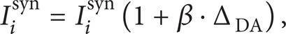
where β is the synaptic efficacy factor and Δ_DA is the dopamine concentration with respect to the default value. We have chosen β = + 0.3 for STR dopamine D1, β = − 0.3 for STR dopamine D2 [20]. Increasing the value of Δ_DA produces a hypersensitivity of the network to a point that, for Δ_DA of the order of 0.5, there is no competition between channels anymore, and all input signals are maximally activated. On the other hand, decreasing the level of tonic dopamine (Δ_DA = − 0.5) produces a system that is less reactive and that filters out all input signals that are not sufficiently high [21].

2.3. The Structure of the SNN in the Robot Behavior Controller

2.3.1. Description of Robot

We consider a wheeled mobile robot with two driving wheels. The sensors around the robot can be classified into three types. The first are ultrasonic ranging (UR) sensors HC-SR04 providing the robot with information on the distance to obstacles located in front of the sensor. There are three sensors, located in the left-front, mid-front, and right-front. The second sensor type is a cadmium sulfide cell, which measures the amount of ambient light. The last type is color sensor TCS230. There are two color sensors located in the front of the robot (left and right sides) and facing frontward.

2.3.2. Encoding the Analog Sensory Information into the Frequency Coding for the SNN's Sensory Neurons

There are several methods to map the intensity of sensory information into spiking neurons, for instance, the frequency code hypothesis, the temporal coincidence hypothesis [22], and the delay coding hypothesis [23]. In this paper, we use the classic frequency method, which maps the stimulus intensity to the firing rate of the neuron. The intensity of the stimulation is represented by the probability that the neuron emits a spike in a time interval. We have taken the firing rate of the motor neurons measured over 20 ms as speed commands to the wheels of the robot.

2.3.3. Simulation Environment and Robot's Task

We establish a three-dimensional T-maze (250 cm × 200 cm) based on ROBOTO shown in Figure 2. The robot starts from the initial position, and it needs to keep away from knocking walls and obstacles and make choices (turn left/right) in several T-intersections in order to ultimately reach the brightest point (light source) position. At each intersection, there is a red bezel or a green bezel on the left or the right, used as the clue signal of the robot.

Figure 2:

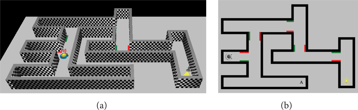
The T-maze environment for the mobile robot. (a) Three-dimensional perspective; (b) top view of 2-dimensional.

2.3.4. The Structure of SNN Controller

Figure 3 shows the structure of the SNN in the controller. There are three groups of sensory information. So in the input layer of the SNN, there are three types of sensory neurons: one light-sensor neuron, two color-sensor neurons, and three UR neurons. The role of UR neuron is to judge whether the opposite obstacle is too close that the robot needs to turn around. The light-sensor neuron is used to detect whether to end searching in the maze. In the hidden layer, there are 40 hidden neurons. These 40 hidden neurons are divided into 2 groups: H1 and H2. Neurons in each set receive the encode stimuli from the corresponding color sensor. In the output layer, there are two motor neurons. The output spikes of the 1st output neuron control the rotating speed of the left wheel and the 2nd output neuron is corresponding to the right wheel.

Figure 3:

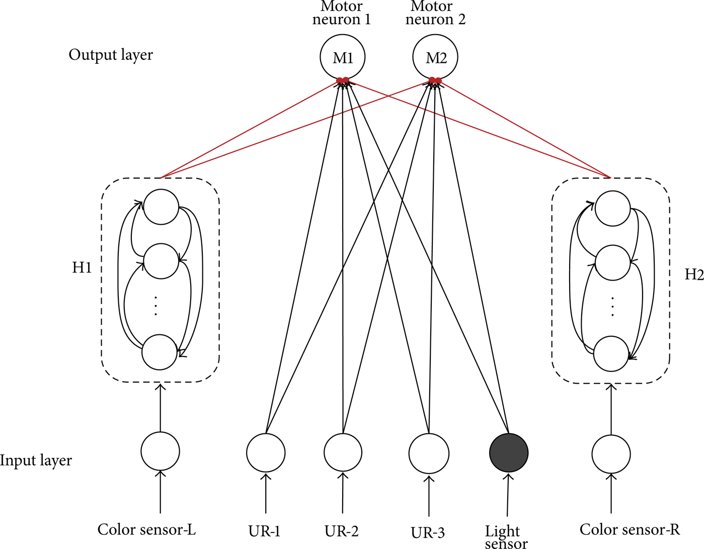
Structure of SNN in the controller. Each neuron in the hidden layer (H1 and H2) is connected to the motor neuron 1 (wheel left) and motor neuron 2 (wheel right), in the output layer. And all these synapses are excitatory.

The whole process is shown in Figure 4. Each time the robot passes through the intersection, the color sensory neurons will generate spikes by the color stimuli. These spikes generate synaptic current through the formation of synapses and stimulate the motor neurons. Assuming that the stimulation time is t _s , statistics the spikes number of the two motor neurons from t _s to t _s + T_ck (T_ck is the time interval for the statistics). If the spike number of M1 neuron is larger than the M2 neuron, it means that the left motor is more active than the right motor so that the speed of the left wheel is greater than that of the right wheel. The robot will turn right in the “T” type intersection; conversely, if the spike number of M2 neuron is greater than the M1 neuron, the robot will turn left; if the spike number of neuron M1 and M2 is equal, the robot chooses a random rotation. An example of the membrane potential and the output spikes of the motor neuron 1 are illustrated in Figure 5. In Figure 5(a), when t = 532.3 ms the membrane potential reached the firing threshold, the motor neuron output spike.

Figure 4:

Flow chart of the mobile robot behavior controller.

Figure 5:

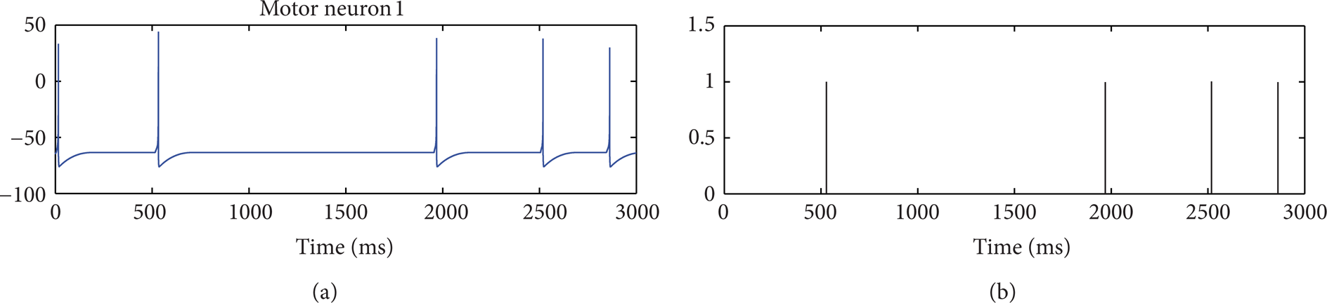
Membrane potential and outputting spikes for the motor neuron. (a) Membrane potential of the motor neuron 1; (b) Outputting spikes of the motor neuron 1.

When the robot comes near the light, the frequency of the spikes coming from the light sensor increases to its maximum and when UR-2 sensor detects the end obstacle, the signals coming from it and the other UR-sensors were not strong enough to reduce it and make the robot stop.

The Specific Equations Used in Figure 4

(a) The “Neuronal Membrane Potential Calculation” Blocks. The calculating formula of each neuron is similar to (1)–(5). The main difference is the current calculation, for example,

• hidden neurons:

  $\begin{array}{l}{\dot{v}}_k=\mathrm{0.04}{v}_k^{\mathrm{2}}+\mathrm{5}{v}_k+\mathrm{140}-u_k+I_k^{\text{syn}}\\ {\dot{u}}_k=a(b{v}_k-u_k)\\ \left(k\in \left[\mathrm{1},N_{\text{hidden}}\right]\right),\end{array}$

  (6)

• where I _k ^syn is the synaptic current from color sensor neurons;

• motor neurons:

  $\begin{array}{c}{\dot{v}}_i=\mathrm{0.04}{v}_i^{\mathrm{2}}+\mathrm{5}{v}_i+\mathrm{140}-u_i+I_{\text{motor}}+{I_i}^{\text{syn}},\\ {\dot{u}}_i=a\left(b{v}_i-u_i\right),\\ I_i^{\text{syn}}=-{\displaystyle \sum }{g}_{li}{s}_l\left(v_i-v_{\text{syn}}\right),\\ \left(i\in \left[\mathrm{1},N_{\text{motor}}\right],l\in \left[\mathrm{1},N_{\text{sensor}}\right],\left[\mathrm{1},N_{\text{hidden}}\right]\right),\end{array}$

  (7)

• where I_motor is the background current for motor neurons (we set I_motor = 3) and I _i ^syn is the synaptic current from sensor neurons and hidden neurons.

(b) The “Complete the Task” Block. The light sensor is a cadmium-sulfide cell 100 mW. It is as photoresistor, where resistance changes based on the incident light. The cell's resistance is inversely proportional to increasing light. The sensor generates an 8-bit value that encodes the light intensity value detected. Its maximum experimental output value is 252 mV, and its minimum is 0 mV. With normal light in the lab, the output was approximately 100 mV; without it the sensors give an output of approximately 10 mV. When the distance from the sensor and light source light_DIS is less than 20 cm, the sensor output light_OUT is greater than 240 mV. As a result, we set the following.

• If light_OUT > 240 then complete target; else not complete target end.

2.4. Simulation Results

2.4.1. Training Process

Figure 6 shows the timing diagram of training process. If the robot turns to the expected direction in a “T” intersection, after a short time, we give awards to the robot by setting Δ_DA = 0.5 in neuron M1 and M2; otherwise, keep the DA concentration unchanged. After several times of training, the robot can memorize the relationship of one specific stimuli, that is, “left-red color and right-green color” or “left-green color and right-red color,” and one specific action, “go left,” “go forward,” or “go right,” forming a sensory-motor contingency.

Figure 6:

Timing diagram of training process.

If the robot goes to a dead end (e.g., point A in Figure 5(b)), the training is over and the robot will reset in the initial position.

2.4.2. Testing Process

Every time the robot goes to the dead end or finds the target (light source) is an individual experiment. A set of experiments includes 50 individual experiments. We do a total of 20 sets of experiments. Figure 7 shows the probability of success (the robot finds the target) relative to the training times. It illustrates that, with the increasing of training times, the probability of the robot to find target increases. After about 60 times of training, the robot is capable of making right choices in all the “T” type intersections and finding the target with the successful rate around 80%.

Figure 7:

The probability curve of the robot to find target successfully with the training times.

3. Hardware Implementation

In this section, we focus on the hardware design, simulation, and implementation of the SNN model onto an FPGA. The approach uses Xilinx System Generator for the simulation and implementation of the neuron models and their networks. The toolboxes we use include Simulink common used blocks, Xilinx blocks, MCode blocks (MATLAB files), and Black Box blocks (Verilog HDL files). The neural network architecture is implemented on the chosen FPGA device, the Altera Cyclone IV EP4CE30F23C6N device.

3.1. Weight Memory

The weight memories are implemented as a whole using an array of Block RAMs, dedicated memory units in the FPGA. Each column of the array implements the weight memory of a slice. The organization and the data ports of the weight memories are shown in Figure 8. A counter is used to generate the address for the weight memories during a spike propagation step. The weights are arranged so they fit with the cycling of the spiking bits as the memory is read.

Figure 8:

The weight memories, implemented altogether as an array of block RAMs. Each column stores the weights for the synapses connecting each neuron of the network to the neuron instantiated by the column. An address in memory, received from the SNN controller block, points to a single bit of a weight value from each column. During spike propagation, this address increments until it reaches the most significant bit of the last weights and is then reset. The loading/unloading block on top of the memory is a serial to parallel register used during initialization and read back.

3.2. Hardware Neuron

Signed floating-point operation is expensive in FPGA implementation; in order to save the resources of FPGA, we vary the Izhikevich model by a linear transformation (8), making it possible to be implemented by the unsigned integer arithmetic.

$\begin{array}{c}\tilde{v}=\mathrm{256}\left(v+\mathrm{90}\right),\\ \tilde{u}=\mathrm{256}\left(u+\mathrm{90}\right).\end{array}$

(8)

Using (1) and (8), we get the following:

$\begin{array}{c}\phantom{\phantom{ooooooooooo}oo}{\dot{\tilde{v}}}_i=\mathrm{0.04}\frac{\mathrm{1}}{\mathrm{256}}{\tilde{v}}_i^{\mathrm{2}}-\mathrm{2.2}{\tilde{v}}_i+\mathrm{26624}-{\tilde{u}}_i+\mathrm{256}I+\mathrm{256}{I}_i^{\text{syn}},\\ {\dot{\tilde{u}}}_i=a\left[b\left({\tilde{v}}_i-\mathrm{23040}\right)-\left({\tilde{u}}_i-\mathrm{23040}\right)\right],\\ \text{if}\hspace{0.17em}{\tilde{v}}_i>\mathrm{256}(\mathrm{30}+\mathrm{90}),\hspace{1em}\text{then}\hspace{0.17em}\hspace{0.17em}\{\begin{array}{cc}{\tilde{v}}_i⟵\mathrm{256}\left(c+\mathrm{90}\right)\hfill & \hfill \\ {\tilde{u}}_i⟵{\tilde{u}}_i+\mathrm{256}d.\hfill & \hfill \end{array}\end{array}$

(9)

We substitute a = 0.02, c = − 65, and d = 8 with (9) and convert all the floating-point number to the fraction whose denominator is the integer power of 2 (e.g., 0.04 = 4/100 ≈ 41/1024),

$\begin{array}{c}\phantom{oo}\phantom{oo}{\dot{\tilde{v}}}_i=\frac{\mathrm{41}}{\mathrm{1024}}\frac{\mathrm{1}}{\mathrm{256}}{\tilde{v}}_i^{\mathrm{2}}-\frac{\mathrm{2253}}{\mathrm{1024}}{\tilde{v}}_i+\mathrm{26624}-{\tilde{u}}_i+\mathrm{256}I+\mathrm{256}{I}_i^{\text{syn}},\\ {\dot{\tilde{u}}}_i=\frac{\mathrm{41}}{\mathrm{2048}}b{\tilde{v}}_i-\mathrm{461}b-\frac{\mathrm{41}}{\mathrm{2048}}{\tilde{u}}_i+\mathrm{461},\\ \text{if}\hspace{0.17em}{\tilde{v}}_i>\mathrm{30720},\hspace{1em}\text{then}\hspace{0.17em}\hspace{0.17em}\{\begin{array}{cc}{\tilde{v}}_i⟵\mathrm{6400}\hfill & \hfill \\ {\tilde{u}}_i⟵{\tilde{u}}_i+\mathrm{2048}.\hfill & \hfill \end{array}\end{array}$

(10)

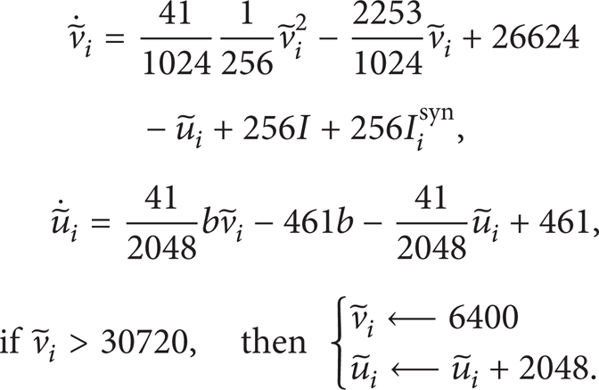
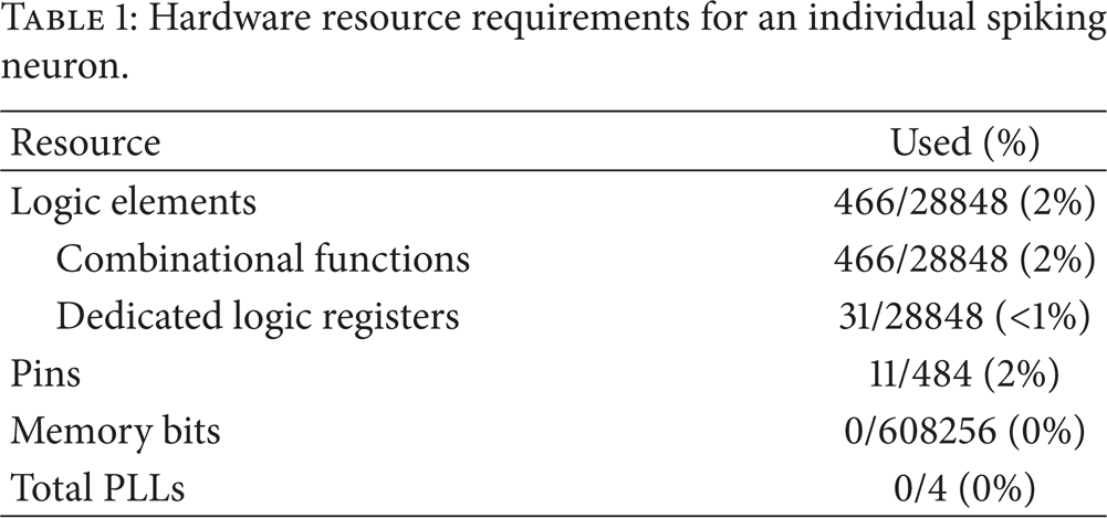
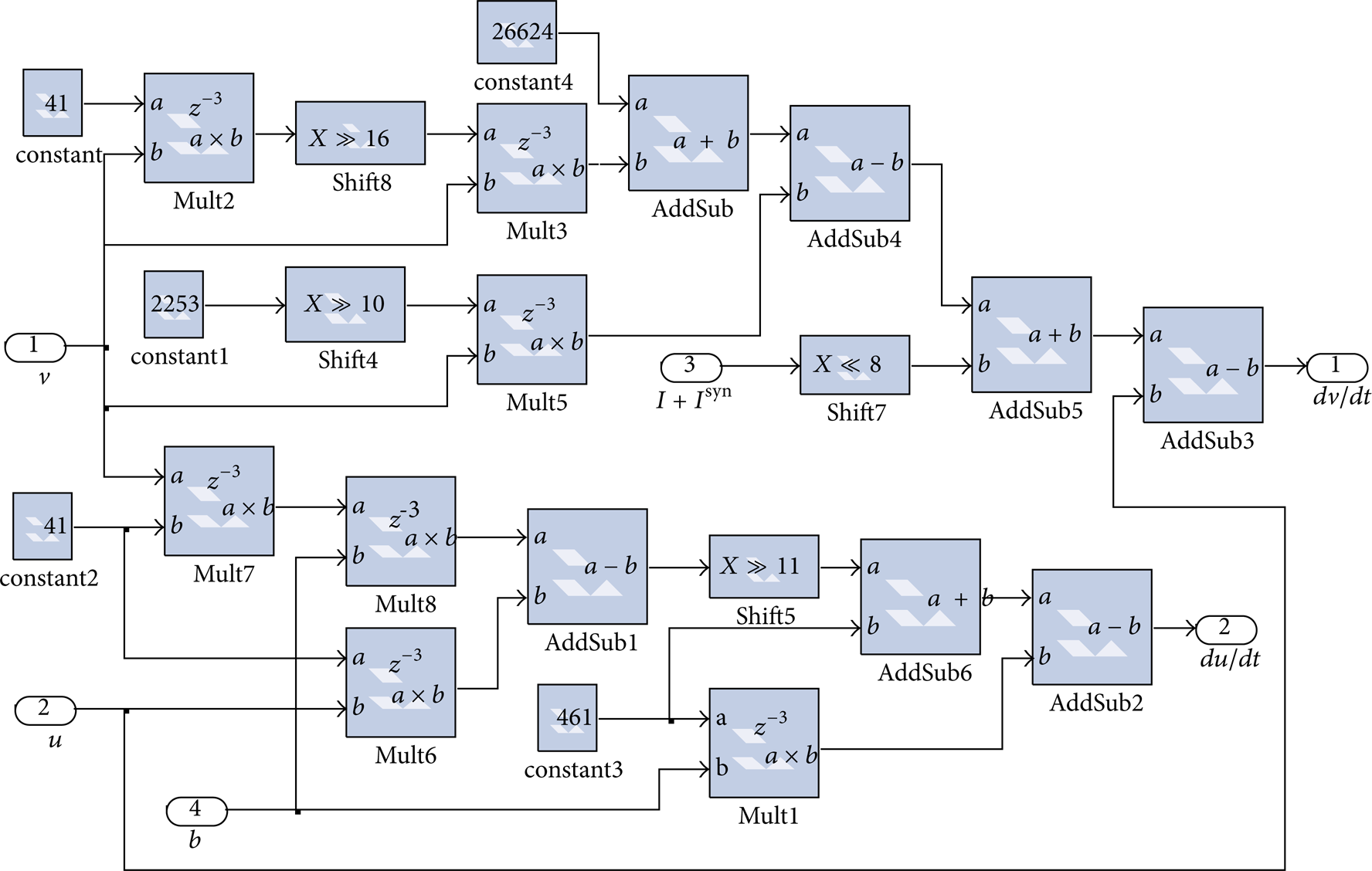
From the converted neuron model (10), we see that an individual neuron can be achieved by multipliers, adders, and shift registers (as shown in Figure 9). A Quartus II report about the utilized resources has been presented in Table 1. Figure 10 shows the testing result simulated on ModelSim.

Table 1:

Hardware resource requirements for an individual spiking neuron.

Resource	Used (%)
Logic elements	466/28848 (2%)
Combinational functions	466/28848 (2%)
Dedicated logic registers	31/28848 (<1%)
Pins	11/484 (2%)
Memory bits	0/608256 (0%)
Total PLLs	0/4 (0%)

Figure 9:

IZH neuron circuit.

Figure 10:

The testing result of the hardware spiking neuron module. The clock signal, current I, and reset signal are the input of the module; the emitting spikes and neuron membrane are the output.

3.3. Learning Module and Synapse Module

For STDP learning, we do a linear transformation (expand 256 times) similar to the neuron model. To save resource, we use a look-up table (LUT) to achieve the function of the exponent calculation formula. The address values in this STDP-LUT are from 0 to 50 (since when Δt > 50 ms, the synaptic modification in (4) is too small). The output values in this STDP-LUT are the values calculated by (4) expanded 256 times.

The synapse block is shown in Figure 11. The “comp_t” block is the STDP-LUT address calculation unit. The necessary commands for this block are the spike signal of the presynaptic/postsynaptic neuron (“pre_spike” and “post_spike”), the clock signal (“clk”). The “stdp_module” is the STDP-LUT unit. “Add” is the address, “read_en” is read control signal, “reset” is the reset signal, and “stdp” is the output signal. The “acc” block is the synaptic current accumulator unit. The necessary commands for this block are the accumulator reset command (re_acc resets the acc when a new computation is made), RAM address (addr_g provides the address of the synaptic weight), synaptic modification (stdp: modification by STDP module), RAM write enable (addr_neuron writes enable signal for neuron which is selected), and the SNN behavioral setting signal (en_str1&en_str2 sets the Dopamine-receptor modulation behaviour).

Figure 11:

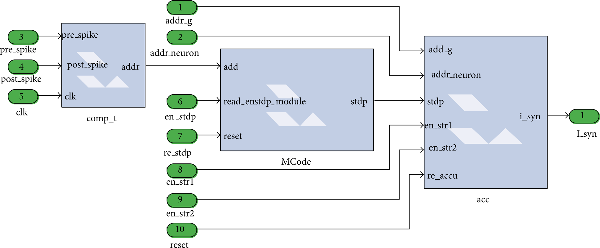
The package of STDP module and synapse module.

3.4. Experiment on a Real Robot

The wheeled mobile robot we used is shown in Figure 12. Its structure is formed by a thin and black plastic piece, upon which can be found the motherboard and all the electronic parts. At each side, there is one wheel and its encoder. It contains the main controller implemented in FPGA (Cyclone IV EP4CE30F23C6N), ultrasonic ranging module (HC-SR04), optical encoder speed module (RB-02S043), and motion control module. Arrays of sensors are located in the peripheral parts (details have been described in Section 2.3.1). Figure 13 shows the real experiment environment for the robot. The walls in the maze are 25 cm high. Experimental result shows that the robot can finally reach the goal after about 100 times training.

Figure 12:

The wheeled mobile robot.

Figure 13:

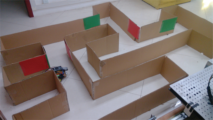
The real maze for experiment.

4. Conclusion

A novel behavior controller for mobile robots based on SNN is designed, and the hardware architecture of this SNN controller with on-chip learning controlled by a generic control unit, described in Verilog HDL code, has been presented. In the controller, the spiking neurons adopt the Izhikevich model, and the synaptic connection in the SNN is tuned by spike timing-dependent plasticity (STDP) learning and dopamine-receptor modulation. The angular velocities of the mobile robot's driving wheels can be controlled by the emitting spikes of the motor neurons directly. The simulation results show that the controller can be used in obstacle avoidance and searching targets in maze successfully. The controller has simple structure and can be implemented easily. Efforts are underway on how to set optimal parameters and select more proper training methods for the SNNs.

Conflict of Interests

The authors declare that there is no conflict of interests regarding the publication of this paper.