Research on Control Method Based on Real-Time Operational Reliability Evaluation for Space Manipulator

Abstract

A control method based on real-time operational reliability evaluation for space manipulator is presented for improving the success rate of a manipulator during the execution of a task. In this paper, a method for quantitative analysis of operational reliability is given when manipulator is executing a specified task; then a control model which could control the quantitative operational reliability is built. First, the control process is described by using a state space equation. Second, process parameters are estimated in real time using Bayesian method. Third, the expression of the system's real-time operational reliability is deduced based on the state space equation and process parameters which are estimated using Bayesian method. Finally, a control variable regulation strategy which considers the cost of control is given based on the Theory of Statistical Process Control. It is shown via simulations that this method effectively improves the operational reliability of space manipulator control system.

1. Introduction

Space manipulator plays a crucial role in construction, recovery, and equipment maintenance of space station and it therefore allays the working time and frequency of astronaut's extravehicular activity. Considering the extreme environment of the space and the difficulty in maintaining, the reliability of space manipulator has become a difficult problem worldwide [1–4]. The inherent reliability of space manipulator decreases continually in service [5], and the control of operational reliability which aims to improve the operational reliability is an economical and effective method to achieve satisfactory performance for space manipulator. Now multiple control methods have been widely used in controlling space manipulator, such as PID control [6], adaptive control [7, 8], variable structure control [9], fuzzy control [10, 11], neural network control [12, 13], and hybrid control [14]. Zhang et al. [6] aimed at trajectory tracking of robot manipulators without velocity information; the study proposed an output feedback PD control without measuring joint velocities dispense with model. Lian [15] developed a self-organizing fuzzy radial basis-function neural network (RBFN) controller (SFRBNC) for robotic systems. The SFRBNC uses an RBFN to regulate in real time these parameters of a self-organizing fuzzy controller to optimal values to achieve satisfactory performance for system control. A new approach combining computed torque control and fuzzy control is developed for trajectory tracking problems of robotic manipulators with structured uncertainty and unstructured uncertainty in [16]. Wai and Muthusamy [17] present the design and analysis of an intelligent control system that inherits the robust properties of sliding-mode control (SMC) for an n-link robot manipulator, including actuator dynamics in order to achieve a high-precision position tracking with a firm robustness. A fuzzy-neural-network inherited SMC scheme is proposed to relax the requirement of detailed system information and deal with chattering control efforts in the SMC system. Chao et al. [18] propose an adaptive tracking control method which can deal with the kinematics uncertainty and uncertainties in both link and actuator dynamics of the rigid-link flexible-joint robot system.

In those control methods, much of the interest was centered on trajectory planning and motion control. No system control model of manipulator has been built considering the effect of operational reliability up to the present, and no method for quantitative analysis of operational reliability has been proposed. On the other hand, the basic idea of current control methods is to regulate control variable when the actual value does not match the expected value in order to do a high-precision position tracking. It means that those control methods are interesting in the performance of a single task and neglect the performance stability of multiple tasks.

All those lead up to a control method based on real-time operational reliability evaluation for space manipulator. This paper introduces the method of maximizing the probability of completing task successfully using an evaluation method of operational reliability in real time and a regulation strategy of control variable.

2. Operational Reliability

The operational reliability of a space manipulator refers to the ability to complete the tasks successfully with specified control methods when it performs specified tasks. The work of space manipulator consists of a collection of a series of tasks, which is denoted by the set T:

$T=\left\{T_i\mid i=\mathrm{1,2},\dots ,n\right\}.$

(1)

For any given task T _i , m factors which determine the success of the task are denoted by I _i :

$I_i=\left\{I_{ij}\mid j=\mathrm{1,2},\dots ,m\right\}.$

(2)

When the task is performed successfully, all the values of I _ij should be positioned in a prescribed accuracy requirement, which is denoted by E _ij :

$E_{ij}=\left[{\lambda }_{ij}-{\epsilon }_{ij},{\lambda }_{ij}+{\epsilon }_{ij}\right],$

(3)

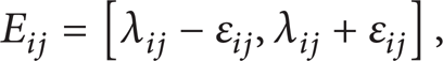
where λ _ij and ε _ij ∈ [0, + ∞) present the expectation and the error allowance of I _ij . So if I _ij ∈ E _ij (i = 1, 2,…, n, j = 1, 2,…, m), when T _i finishes, then task T _i is successful; otherwise it fails. Now a random variable X _ij is used to describe the value of I _ij ; at the end of the task execution, the distribution function of X _ij can be written as follows:

$F_{ij}\left({\lambda }_{ij}\right)=P\left\{X_{ij}<{\lambda }_{ij}\right\},\hspace{1em}j=\mathrm{1,2},\dots ,m.$

(4)

On this basis, the probability of X _ij meeting the accuracy requirements of task T _i can be expressed as follows:

$R\left(E_{ij}\right)=P\left\{{\displaystyle \bigcap }_{j=\mathrm{1}}^m{X}_{ij}\in E_{ij}\right\},$

(5)

where R(E _ij ) is the operational reliability of the space manipulator. By formula (5), it is known that operational reliability of a manipulator is the probability that each factor meets specified accuracy requirement when it performs a task. Therefore, the operational reliability of a space manipulator can also be defined as follows: the probability of successful completing specified task when using specified control method to control the manipulator. So I _ij can be called the factors influencing the operational reliability as well, and it may be the pose, velocity, or force output of the end of manipulator or some other parameters of the manipulator according to different tasks.

3. Control Model of Operational Reliability

As is shown in Figure 1, this paper presents a control model of operational reliability for manipulator. In this model, the operational reliability of the control system is considered by adding a feedback channel in order to do a closed-loop operational reliability control of the system while the manipulator is executing a specified task T _i .

Figure 1:

Block diagram of control model of operational reliability.

Under normal conditions there is no fault in the manipulator; the first step is Task Planning, including the following steps.

1. Carry out profile analysis of the specified task and identify constraints and optimization criteria in the process of movement.

2. According to the optimization criteria of the task, it is divided into several task stages.

3. Judge whether the task stage division is feasible or whether position violates the constraints or not, and output the task's intermediate point finally.

Then, trajectory planning will be called according to the intermediate point of the task, including the following steps.

1. Establish the optimization objective function.

2. Use a search algorithm to search the optimal path of the space manipulator.

Finally, the Optimal Motion Control Strategy is used to execute the trajectory planning scheme considering the dynamic time-varying constraints.

In the running process of manipulator, the operational reliability R(E _ij ) is evaluated in real time based on the current state of system. Then the evaluated R(E _ij ) is compared with the operational reliability which the task is required to meet; if R(E _ij ) is less than the task's requirement, whether control variables need to be regulated is decided by an Regulation Strategy of Control Variable, and the regulation of control variable is also calculated by that regulation strategy. Finally, the regulation superposes on the input of motion control, and the manipulator is controlled with the use of this new control variable. It makes the execution result of manipulator more similar to the trajectory planning scheme. Thus, the probability of completing task successfully is improved.

Under fault conditions, system fault which includes the source of fault and other related information is detected by Fault Diagnosis Module based on the information which provided by System Condition Detection Module. Then, Fault Self-Handling Module and Model Reconstruction Module are called to deal with the system fault, and Task Planning is recalled to continue the task.

According to the control model of operational reliability presented in the paper, the Task Planning scheme which is feasible and costs minimum is produced, and then system's noise and environment's disturbance are taken into consideration during the execution of the task so that execution result is more probably the same as the scheme of Task Planning. These can guarantee the maximum probability of completing the task successfully and the minimum cost of execution at the same time. Thus the operational reliability of the manipulator is improved.

4. Application of Control Method

According to the application of space manipulator in orbit, service tasks of space manipulator in orbit are typically divided into four tasks: transfer without load, transfer with load, capture, and assemble. More complex task consists of these four types of typical tasks [19–22]. In this paper, “transfer without load” task is used as an example to illustrate the realization of control method of operational reliability. “Transfer without load” refers to the transition motion of manipulator between two different configurations without load, mainly in the service of the following conditions: manipulator's opening from pressed state, preadjustment of configuration before performing a task, manipulator retracement, and other events after the completion of a task. In “transfer without load” task, only the accuracy of terminal position determines the success of the task, whose typical control variable is the angle of each joint.

In the process of task execution, angle information of each joint is obtained through sensors. The general expression of connecting rod transformation matrix ${}_i{}^{i-\mathrm{1}}T$ about coordinate {i} relative to coordinate {i − 1} can be acquired according to the D-H parameters and transformation relation between coordinate systems:

${}_i{}^{i-\mathrm{1}}T=\left[\begin{array}{cc}\begin{array}{cc}c{\theta }_i& -s{\theta }_i\\ s{\theta }_{i}c{\alpha }_{i-\mathrm{1}}& c{\theta }_{i}c{\alpha }_{i-\mathrm{1}}\end{array}& \begin{array}{cc}\mathrm{0}& a_{i-\mathrm{1}}\\ s{\alpha }_{i-\mathrm{1}}& -d_{i}s{\alpha }_{i-\mathrm{1}}\end{array}\\ \begin{array}{cc}s{\theta }_{i}s{\alpha }_{i-\mathrm{1}}& c{\theta }_{i}c{\alpha }_{i-\mathrm{1}}\\ \mathrm{0}& \mathrm{0}\end{array}& \begin{array}{cc}c{\alpha }_{i-\mathrm{1}}& d_{i}c{\alpha }_{i-\mathrm{1}}\\ \mathrm{0}& \mathrm{1}\end{array}\end{array}\right].$

(6)

And the transformation matrix of the ending connecting rod coordinate system {n} relative to coordinate system {0} is as follows:

${}_n{}^{\mathrm{0}}T={}_{\mathrm{1}}{}^{\mathrm{0}}T{}_{\mathrm{2}}{}^{\mathrm{1}}T{}_{\mathrm{3}}{}^{\mathrm{2}}T\cdots {}_n{}^{n-\mathrm{1}}T=\left(\begin{array}{cc}{}_n{}^{\mathrm{0}}R& {}_{\mathrm{\hspace{0.17em}\hspace{0.17em}}}{}^{\mathrm{0}}P\\ \begin{array}{cc}0& 0\end{array}& \begin{array}{cc}0& 1\end{array}\end{array}\right),$

(7)

where position vector P represents the position of the ending connecting rod and the rotation matrix R = [n o a] represents its attitude. The relationship between the pose of the ending connecting rod and the joint angles can be established based on ${}_n{}^{\mathrm{0}}T$ . The end position of manipulator in the base coordinate system is represented by

$r_o={}^{\mathrm{0}}{P}^T={\left(d_x\mathrm{\hspace{0.17em}\hspace{0.17em}}{d}_y\mathrm{\hspace{0.17em}\hspace{0.17em}}{d}_z\right)}^T.$

(8)

Every moment the target end position r _t of manipulator in the motion process is from Task Planning and trajectory planning algorithm; the observed error of end position is noted by y which is obtained through sensors with noises; and the true error of ending position is represented by θ:

$\begin{array}{c}y=r_o-r_t,\\ \theta =r_r-r_t,\end{array}$

(9)

where r _o notes the observed end position which is calculated though forward kinematics according to the joint angles detected by sensors and r _r is the true end position of the manipulator.

Compared with θ, y has noises due to the manufacturing errors, assembling errors, and environment disturbance. Therefore, y, calculated based on the information from sensors, cannot reflect the true value. Taking y as the training samples, parameter θ which is used to calculate the current operational reliability of system according to formula (5) is evaluated based on Bayesian method. After that, the current operational reliability of system is calculated and is used to compare with the preset goal of the task. If the current operational reliability is less than the task's requirements, the regulation is calculated for the end position under the condition of θ which is evaluated by Bayesian method. Finally, the regulations of each joint angle which is used to revise the control of manipulator are calculated by inverse kinematics.

4.1. Mathematical Description of the Control Process

For the closed-loop control system of manipulator, the state space equations to describe the control process can be expressed as follows:

$\begin{array}{l}{\theta }_i={\theta }_{i-\mathrm{1}}+x_{i-\mathrm{1}},\\ y_i={\theta }_i+v_i,\\ i=\mathrm{1,2},\dots ,N,\end{array}$

(10)

where θ _i = (d _ix ′, d _iy ′, d _iz ′) ^T presents the value of reliability affecting factors—the actual terminal position error for the ith control cycle; y _i = (d _ix , d _iy , d_iz) ^T presents the observed value of reliability affecting factors, namely, the terminal position error obtained by forward kinematics solution with the noise for the ith control cycle; x _i = (Δd _ix , Δd _iy , Δd _iz ) ^T presents the calculated regulation amount of control variable for the ith control cycle; the observation error fluctuation v _i obeys Gaussian distribution v _i ∼N(0, Σ).

Dimensionalities of θ _i , y _i , x _i , and v _i in formula (10) are all equal.

4.2. Operational Reliability Evaluation

Some unknown parameters in the state space equations need to be estimated online according to the process of task. According to each parameter's prior distribution in the state space equations and y _i detected in each control cycle, their posterior distribution are deduced by the Bayesian formula. As the posterior distribution of the actual terminal position error θ _i is obtained, namely, the probability density function f(θ _i ∣ y _i ), the system's real-time operational reliability is calculated according to formula (5).

4.2.1. Parameter Estimation

The basic idea of Bayesian estimation is that all unknown variables are regarded as random variables and are estimated by Bayes theorem combined with the cognitive status of unknown variables and data information obtained from reality. In this paper, we use Bayesian method to infer the unknown parameter θ₀ of the process and adjust the process accordingly. On this basis, the normal conjugate prior model can be written as follows:

$\begin{array}{c}{\theta }_{\mathrm{0}}~N_p\left({\mu }_{\mathrm{0}},{\Lambda }_{\mathrm{0}}\right),\\ y_{\mathrm{1}}\mid {\theta }_{\mathrm{0}}~N_p\left({\theta }_{\mathrm{0}}+x_{\mathrm{0}},\Sigma \right).\end{array}$

(11)

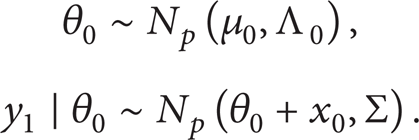
According to the Bayesian method it is obtained that

$p\left({\theta }_{\mathrm{0}}\mid y_{\mathrm{1}}\right)=\frac{p\left(y_{\mathrm{1}}\mid {\theta }_{\mathrm{0}}\right)p\left({\theta }_{\mathrm{0}}\right)}{\int p\left(y_{\mathrm{1}}\mid {\theta }_{\mathrm{0}}\right)p\left({\theta }_{\mathrm{0}}\right)d{\theta }_{\mathrm{0}}}.$

(12)

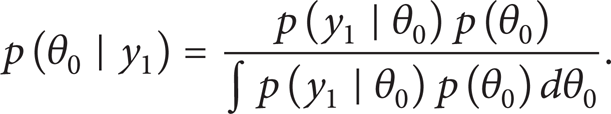
When it is solved, the distribution of θ₀ ∣ y₁ is obtained:

${\theta }_{\mathrm{0}}\mid y_{\mathrm{1}}~N_p\left(\frac{{\Sigma }^{-\mathrm{1}}\left(y_{\mathrm{1}}-x_{\mathrm{0}}\right)+{\Lambda }_{\mathrm{0}}^{-\mathrm{1}}{\mu }_{\mathrm{0}}}{{\Sigma }^{-\mathrm{1}}+{\Lambda }_{\mathrm{0}}^{-\mathrm{1}}},\frac{{\Sigma \Lambda }_{\mathrm{0}}}{\Sigma +{\Lambda }_{\mathrm{0}}}\right).$

(13)

By θ _i = θ_{i − 1} + x_{i − 1}, it is obtained that

${\theta }_{\mathrm{1}}\mid y_{\mathrm{1}}~N_p\left({\mu }_{\mathrm{1}},{\Lambda }_{\mathrm{1}}\right),$

(14)

$\begin{array}{c}{\mu }_{\mathrm{1}}={\mu }_{\mathrm{1}}^{\prime }+x_{\mathrm{0}}=\frac{{\Sigma }^{-\mathrm{1}}\left(y_{\mathrm{1}}-x_{\mathrm{0}}\right)+{\Lambda }_{\mathrm{0}}^{-\mathrm{1}}{\mu }_{\mathrm{0}}}{{\Sigma }^{-\mathrm{1}}+{\Lambda }_{\mathrm{0}}^{-\mathrm{1}}}+x_{\mathrm{0}}\\ \hspace{1em}\hspace{1em}\hspace{1em}=\frac{{\Sigma }^{-\mathrm{1}}{y}_{\mathrm{1}}+{\Lambda }_{\mathrm{0}}^{-\mathrm{1}}\left({\mu }_{\mathrm{0}}+x_{\mathrm{0}}\right)}{{\Sigma }^{-\mathrm{1}}+{\Lambda }_{\mathrm{0}}^{-\mathrm{1}}}.\end{array}$

(15)

On the basis of iteration it is obtained for the a posteriori distribution of actual terminal position error θ _i for the ith control cycle that

${\theta }_i\mid y_i~N_p\left({\mu }_i,{\Lambda }_i\right),$

(16)

where

$\begin{array}{c}{\mu }_i=\frac{{\Sigma }^{-\mathrm{1}}{y}_i+{\Lambda }_{i-\mathrm{1}}^{-\mathrm{1}}\left({\mu }_{i-\mathrm{1}}+x_{i-\mathrm{1}}\right)}{{\Sigma }^{-\mathrm{1}}+{\Lambda }_{i-\mathrm{1}}^{-\mathrm{1}}},\\ {\Lambda }_i=\frac{{\Sigma \Lambda }_{i-\mathrm{1}}}{\Sigma +{\Lambda }_{i-\mathrm{1}}}.\end{array}$

(17)

Prior distribution of the output value for the (i + 1) th control cycle is y_{i + 1} ∣ θ _i ∼N _p (θ _i + x _i , Σ).

After completing the regulation for the ith control cycle, the probability density function of y_{i + 1} ∣ y _i , x _i for the (i + 1) th control cycle can be written as follows:

$p\left(y_{i+\mathrm{1}}\mid y_i,x_i\right)={\displaystyle \int }p\left(y_{i+\mathrm{1}}\mid {\theta }_i\right)p\left({\theta }_i\mid y_i,x_i\right)d{\theta }_i.$

(18)

Because p(y_{i + 1} ∣ y _i , x _i ) obeys normal distribution, so the posteriori distribution of y_{i + 1} can be expressed as follows:

$y_{i+\mathrm{1}}\mid y_i~N\left(x_i+{\mu }_i,{\Lambda }_i+\Sigma \right).$

(19)

According to formula (17) it can be also obtained that

${\mu }_i\mid y_{i-\mathrm{1}}~N(\phantom{{\left({\left({\Sigma }^{-\mathrm{1}}+{\Lambda }_{i-\mathrm{1}}^{-\mathrm{1}}\right)}^{-\mathrm{1}}{\Sigma }^{-\mathrm{1}}\right)}^T}{x}_{i-\mathrm{1}}+{\mu }_{i-\mathrm{1}},{\left({\Sigma }^{-\mathrm{1}}+{\Lambda }_{i-\mathrm{1}}^{-\mathrm{1}}\right)}^{-\mathrm{1}}{\Sigma }^{-\mathrm{1}}·\left({\Lambda }_{i-\mathrm{1}}+\Sigma \right){\left({\left({\Sigma }^{-\mathrm{1}}+{\Lambda }_{i-\mathrm{1}}^{-\mathrm{1}}\right)}^{-\mathrm{1}}{\Sigma }^{-\mathrm{1}}\right)}^T).$

(20)

4.2.2. Operational Reliability of System in Real Time

According to the expression of the operational reliability in Section 2, the real-time operational reliability for the ith control cycle is a posteriori probability of the actual terminal position error θ _i falling within a prescribed range. According to formulas (16) and (17), the probability density function of θ _i ∣ y _i can be written as follows:

$f\left({\theta }_i\mid y_i\right)=\frac{\mathrm{1}}{\sqrt{\mathrm{2}\pi {\Lambda }_i}}\exp \left\{-\left[\frac{{\left({\theta }_i-{\mu }_i\right)}^{\mathrm{2}}}{\mathrm{2}{\Lambda }_i}\right]\right\}.$

(21)

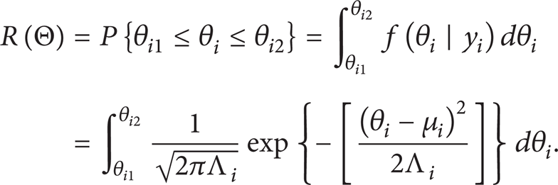
Precision range is prescribed for θ = [θ_i1, θ_i2], where θ_i1 is the precision threshold's lower limit and θ_i2 is the precision threshold's upper limit. According to formula (5), the system's current operational reliability is obtained:

$\begin{array}{c}R\left(\Theta \right)=P\left\{{{\theta }_{i\mathrm{1}}\le \theta }_i\le {\theta }_{i\mathrm{2}}\right\}={{\displaystyle \int }}_{{\theta }_{i\mathrm{1}}}^{{\theta }_{i\mathrm{2}}}f\left({\theta }_i\mid y_i\right)d{\theta }_i\\ ={{\displaystyle \int }}_{{\theta }_{i\mathrm{1}}}^{{\theta }_{i\mathrm{2}}}\frac{\mathrm{1}}{\sqrt{\mathrm{2}\pi {\Lambda }_i}}\exp \left\{-\left[\frac{{\left({\theta }_i-{\mu }_i\right)}^{\mathrm{2}}}{\mathrm{2}{\Lambda }_i}\right]\right\}d{\theta }_i.\end{array}$

(22)

4.3. Optimal Regulation Strategy

4.3.1. Performance Function of Control Process

Due to the existence of disturbance and noise of each link in the control system, excessive regulation of control variables will bring more disturbances into the system when the actual error of terminal position is within the preset accuracy requirement. And the resulting loss of accuracy is defined as regulation costs. According to [23], the performance function is expressed as follows:

$L=E\left[{\displaystyle \sum }_{i=\mathrm{1}}^N{y_i}^T{y}_i+c\delta \left(x_{i-\mathrm{1}}\right)\right],$

(23)

where E[·] is the mathematical expectation; c is the normalized regulation costs; and the formula of δ(x) is defined as follows:

$\delta \left(x\right)=\{\begin{array}{cc}\mathrm{1},\hfill & x\ne \mathrm{0}\hfill \\ \mathrm{0},\hfill & x=\mathrm{0}.\hfill \end{array}$

(24)

Therefore, considering the condition of the terminal position error and regulation costs at the same time, the optimum control strategy for manipulator is the regulation quantity sequence of control variable {x _i , i = 1, 2, 3,…, N} when the value of performance function L reaches the minimum.

4.3.2. Regulation Strategy

For convenient expression of the formula, make y _i = (d _ix , d _iy , d _iz ) ^T = (y_i1, y_i2, y_i3,) ^T ; L _i ^*(μ _i ) is the minimal expected losses from the (i + 1) th cycle to the end when the deviation for the ith cycle is μ _i , while L _i (μ _i ) denotes the minimal expected losses from the (i + 1) th cycle to the end without regulation when the deviation for the ith cycle is μ _i .

(1) Considering the Value of L _i ^*(μ _i ) When i = N − 1. When i = N − 1, namely, after the completion of the (N − 1) th cycle, the minimal expected loss of quality is written as follows:

$\begin{array}{l}{L}_{N-\mathrm{1}}^{*}\left({\mu }_{N-\mathrm{1}}\right)=\underset{x_{N-\mathrm{1}}}{\min }\left\{E\left[y_N^T{y}_N+c\delta \left(x_{N-\mathrm{1}}\right)\right]\right\}\\ \hspace{1em}\hspace{1em}\hspace{1em}\hspace{0.17em}=\underset{x_{N-\mathrm{1}}}{\min }\{{\displaystyle \sum }_{j=\mathrm{1}}^{\mathrm{3}}\left[E^{\mathrm{2}}\left(y_{Nj}\right)+\mathrm{Var}\left(y_{Nj}\right)\right]\hspace{1em}+c\delta \left(x_{N-\mathrm{1}}\right)\}.\end{array}$

(25)

And because of formula (19), it is obtained that

$L_{N-\mathrm{1}}^{*}\left({\mu }_{N-\mathrm{1}}\right)=\mathrm{tr}\left(\Sigma +{\Lambda }_{N-\mathrm{1}}\right)+\underset{x_{N-\mathrm{1}}}{\min }\left\{{\parallel {\mu }_{N-\mathrm{1}}\parallel }^{\mathrm{2}},c\right\}.$

(26)

From above the adjustment boundary ∥μ_{N − 1}∥² > c is obtained; namely, the optimal adjustment strategy after the (N − 1) th control cycle is expressed as follows:

$x_{N-\mathrm{1}}=\{\begin{array}{cc}-{\mu }_{N-\mathrm{1}},\hfill & {\parallel {\mu }_{N-\mathrm{1}}\parallel }^2>c\hfill \\ 0,\hfill & {\parallel {\mu }_{N-\mathrm{1}}\parallel }^2\le c.\hfill \end{array}$

(27)

(2) Considering the Value of L _i ^*(μ _i ) When i ∈ [0, N − 1). Next the minimal expected loss L _i ^*(μ _i ) when i ∈ [0, N − 1) is considered, which will be written as the following recursion:

$L_i^{*}\left({\mu }_i\right)=\underset{x_i}{\min }\{\phantom{+{\displaystyle \int }{L}_{i+\mathrm{1}}^{*}\left({\mu }_{i+\mathrm{1}}\right)f\left({\mu }_{i+\mathrm{1}}{y}_i,x_i\right)d{\mu }_{i+\mathrm{1}}}{\parallel {\mu }_i+x_i\parallel }^{\mathrm{2}}+\mathrm{tr}\left(\Sigma +{\Lambda }_i\right)+c\delta \left(x_i\right)+{\displaystyle \int }{L}_{i+\mathrm{1}}^{*}\left({\mu }_{i+\mathrm{1}}\right)f\left({\mu }_{i+\mathrm{1}}\mid y_i,x_i\right)d{\mu }_{i+\mathrm{1}}\},$

(28)

where f(·) is the probability density function; it leads to

$L_{N-\mathrm{2}}^{*}\left({\mu }_{N-\mathrm{2}}\right)=\mathrm{tr}\left(\Sigma +{\Lambda }_{N-\mathrm{2}}\right)+\mathrm{tr}\left(\Sigma +{\Lambda }_{N-\mathrm{1}}\right)+c+\underset{x_{N-\mathrm{2}}}{\min }\{{\parallel {\mu }_{N-\mathrm{2}}+x_{N-\mathrm{2}}\parallel }^{\mathrm{2}}+c\delta \left(x_{N-\mathrm{2}}\right)+{{\displaystyle \int }}_{\left[{\parallel {\mu }_{N-\mathrm{1}}\parallel }^{\mathrm{2}}<c\right]}\left({\parallel {\mu }_{N-\mathrm{1}}\parallel }^{\mathrm{2}}-c\right)·f\left({\mu }_{N-\mathrm{1}}\mid y_{N-\mathrm{2}},x_{N-\mathrm{2}}\right)d{\mu }_{N-\mathrm{1}}\phantom{{\parallel {\mu }_{N-\mathrm{2}}+x_{N-\mathrm{2}}\parallel }^{\mathrm{2}}+c\delta \left(x_{N-\mathrm{2}}\right)}\}.$

(29)

According to the mean value theorem of integrals, a μ_{N − 1}⁰ ∈ [∥μ_{N − 1}∥² < c] is obtained satisfying

$\begin{array}{c}{{\displaystyle \int }}_{\left[{\parallel {\mu }_{N-\mathrm{1}}\parallel }^{\mathrm{2}}<c\right]}\left({\parallel {\mu }_{N-\mathrm{1}}\parallel }^{\mathrm{2}}-c\right)f\left({\mu }_{N-\mathrm{1}}\mid y_{N-\mathrm{2}},x_{N-\mathrm{2}}\right)d{\mu }_{N-\mathrm{1}}\\ \hspace{1em}\hspace{1em}={\left({\parallel {\mu }_{N-\mathrm{1}}^{\mathrm{0}}\parallel }^{\mathrm{2}}-c\right)}_{\left[{\parallel {\mu }_{N-\mathrm{1}}\parallel }^{\mathrm{2}}<c\right]}\\ \hspace{1em}\hspace{1em}\hspace{1em}\hspace{1em}·{{\displaystyle \int }}_{\left[{\parallel {\mu }_{N-\mathrm{1}}\parallel }^{\mathrm{2}}<c\right]}f\left({\mu }_{N-\mathrm{1}}\mid y_{N-\mathrm{2}},x_{N-\mathrm{2}}\right)d{\mu }_{N-\mathrm{1}}.\end{array}$

(30)

Based on formula (20), it is obtained that

${\mu }_{N-\mathrm{1}}\mid Y^{N-\mathrm{2}},X^{N-\mathrm{2}}~N(\phantom{{\left({\left({\Lambda }_{N-\mathrm{2}}^{-\mathrm{1}}+{\Sigma }^{-\mathrm{1}}\right)}^{-\mathrm{1}}{\Sigma }^{-\mathrm{1}}\right)}^T}{\mu }_{N-\mathrm{2}}+x_{N-\mathrm{2}},{\left({\Lambda }_{N-\mathrm{2}}^{-\mathrm{1}}+{\Sigma }^{-\mathrm{1}}\right)}^{-\mathrm{1}}·{\Sigma }^{-\mathrm{1}}\left({\Lambda }_{N-\mathrm{2}}+\Sigma \right)·{\left({\left({\Lambda }_{N-\mathrm{2}}^{-\mathrm{1}}+{\Sigma }^{-\mathrm{1}}\right)}^{-\mathrm{1}}{\Sigma }^{-\mathrm{1}}\right)}^T).$

(31)

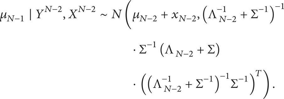
Due to the integrating range [∥μ_{N − 1}∥² < c] being symmetrical about μ_{N − 1} = 0 and f(μ_{N − 1} ∣ y_{N − 2}, x_{N − 2}) obeying normal distribution with the expectation of μ_{N − 2} + x_{N − 2} according to formula (30) the minimum value when μ_{N − 2} + x_{N − 2} = 0, that is, x_{N − 2} = − μ_{N − 2}, then L_{N − 2}^*(μ_{N − 2}) is obtained:

$\begin{array}{c}{L}_{N-\mathrm{2}}^{*}\left({\mu }_{N-\mathrm{2}}\right)\\ =\underset{x_{N-\mathrm{2}}}{\min }\{\phantom{{\displaystyle \int }}\mathrm{tr}\left(\Sigma +{\Lambda }_{N-\mathrm{2}}\right)+{\parallel {\mu }_{N-\mathrm{2}}\parallel }^{\mathrm{2}}+{\displaystyle \int }{L}_{N-\mathrm{1}}^{*}\left({\mu }_{N-\mathrm{1}}\right)f\left({\mu }_{N-\mathrm{1}}\mid y_{N-\mathrm{2}},x_{N-\mathrm{2}}=\mathrm{0}\right)·d{\mu }_{N-\mathrm{1}},\mathrm{tr}\left(\Sigma +{\Lambda }_{N-\mathrm{2}}\right)+c+{\displaystyle \int }{L}_{N-\mathrm{1}}^{*}\left({\mu }_{N-\mathrm{1}}\right)f\left({\mu }_{N-\mathrm{1}}\mid y_{N-\mathrm{2}},{x_{N-\mathrm{2}}=-\mu }_{N-\mathrm{2}}\right)·d{\mu }_{N-\mathrm{1}}\phantom{\mathrm{tr}\left(\Sigma +{\Lambda }_{N-\mathrm{2}}\right)+{\displaystyle \int }{\parallel {\mu }_{N-\mathrm{2}}\parallel }^{\mathrm{2}}}\}\\ \hspace{1em}\hspace{1em}=\underset{x_{N-\mathrm{2}}}{\min }\left\{L_{N-\mathrm{2}}\left({\mu }_{N-\mathrm{2}}\right),c+L_{N-\mathrm{2}}\left(\mathrm{0}\right)\right\}.\end{array}$

(32)

Now it is supposed that

$L_i^{*}\left({\mu }_i\right)=\min \left\{L_i\left({\mu }_i\right),c+L_i\left(\mathrm{0}\right)\right\}.$

(33)

It has been proved that the above formula sets up when i = N − 1, N − 2, and it could be easily proved when it is the (i − 1) th control cycle. Using the mathematical induction, it is easily proved that formula (33) is founded.

Thus it can be written as follows:

$x_i\left({\mu }_i\right)=\{\begin{array}{cc}-{\mu }_i,\hfill & {\parallel {\mu }_i\parallel }^{\mathrm{2}}>{\left({\mu }_i^{*}\right)}^{\mathrm{2}},\hfill \\ \mathrm{0},\hfill & {\parallel {\mu }_i\parallel }^{\mathrm{2}}\le {\left({\mu }_i^{*}\right)}^{\mathrm{2}},\hfill \end{array}$

(34)

where μ _i ^* is the ∥μ _i ∥ satisfying the equation L _i (μ _i ) = c + L _i (0). Obviously, the bigger the μ _i is, the greater the loss of accuracy is. L _i (μ _i ) increases monotonically with increasing μ _i . Therefore, the regulation boundary μ _i ^* for L _i (μ _i ) is the ∥μ _i ∥ satisfying the equation L _i (μ _i ) = c + L _i (0).

According to the equation above, the control process is regulated through updating μ _i based on the observation vector y _i , after the ith cycle has been completed. Then, ∥μ _i ∥ is used to compare with μ _i ^*. And regulation will take place if ∥μ _i ∥² > (μ _i ^*)². It could be noted that the regulation limit is not constant but varies with the cycle i.

4.3.3. Determination of Adjustment Boundary

According to formula (34), for any stage in the process of control, the equation L _i (μ _i ) = c + L _i (0) is to be solved. The solution of unknown variables μ _i is the regulation boundary. Based on formulas (17), (20), (28), and (33), the recursive equations with regulation boundary as the unknown are expressed as follows:

$\begin{array}{c}{L}_i\left({\mu }_i\right)=c+L_i\left(\mathrm{0}\right),\\ L_i\left({\mu }_i\right)=L_i^{*}\left({\mu }_i,x_i=\mathrm{0}\right),\\ L_i^{*}\left({\mu }_i\right)=\min \left\{L_i\left({\mu }_i\right),c+L_i\left(\mathrm{0}\right)\right\},\\ L_i^{*}\left({\mu }_i\right)=\underset{x_i}{\min }\{\phantom{+{\displaystyle \int }{L}_{i+\mathrm{1}}^{*}\left({\mu }_{i+\mathrm{1}}\right)f\left({\mu }_{i+\mathrm{1}}{y}_i,x_i\right)d{\mu }_{i+\mathrm{1}}}{\parallel {\mu }_i+x_i\parallel }^{\mathrm{2}}+\mathrm{tr}\left(\Sigma +{\Lambda }_i\right)+c\delta \left(x_i\right)+{\displaystyle \int }{L}_{i+\mathrm{1}}^{*}\left({\mu }_{i+\mathrm{1}}\right)f\left({\mu }_{i+\mathrm{1}}\mid y_i,x_i\right)d{\mu }_{i+\mathrm{1}}\}.\end{array}$

(35)

In the actual control, the equation is solved by numerical method, discretizing μ _i within the ± 3σ range of its distribution and determining the precision according to actual needs. For each discrete value L _i (μ _i ) and c + L _i (0) are calculated, respectively, and the discrete value of μ _i satisfying the minimum of L _i (μ _i ) − c + L _i (0) is taken as the regulation boundary.

5. Performance Analysis

5.1. Simulation for Single Task

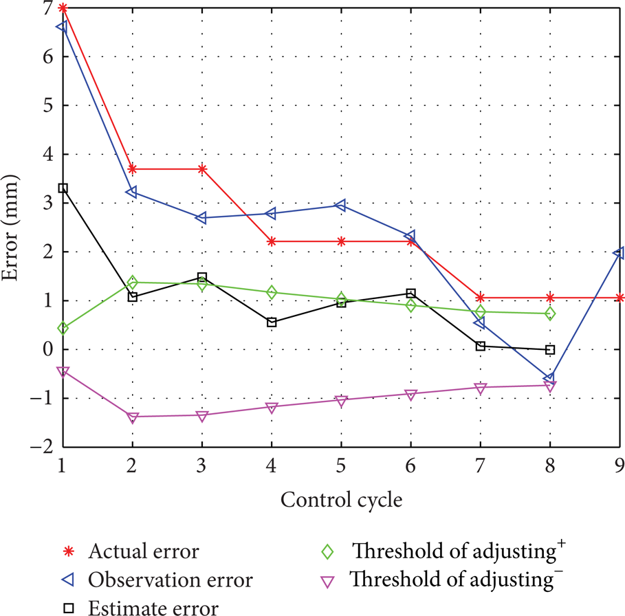
In this section, we first resort to a simulation to demonstrate the performance of the “transfer without load” task with and without application of the Control Method of Operational Reliability. The accuracy and reliability requirement of the task are, respectively, set as ± 1 mm and 0.9. The initial error of end position is set as 7 mm; the true error of end position is assumed to the distribution θ₀∼N(0, 1). Further, we introduce noise v₀ in the error of end position and assume that the noise obeys a Gaussian distribution v₀∼N(0, 1). The task was executed once with and without application of the Control Method of Operational Reliability, respectively. In Figures 2, 3, and 4, the abscissa represents the control cycle, while the ordinate represents the terminal error, using the unit of mm.

Figure 2:

Accuracy in a single task using control method of operational reliability.

Figure 3:

Changing curve of operational reliability in a single task using control method of operational reliability.

Figure 4:

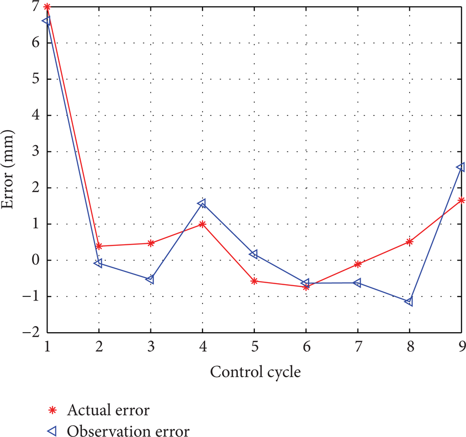
Accuracy in a single task without using control method of operational reliability.

Figure 2 shows the accuracy in a single task using control method of operational reliability. The estimation value of the manipulator's error gradually converged to its true error. The control variable was regulated, respectively, at the 1st, 2nd, and 6th cycles in the whole control process. Also, the true error gradually converged to zero smoothly and with no fluctuation.

Figure 3 shows the changing curve of operational reliability in a single task using control method of operational reliability. It could be observed that the operational reliability of the system showed an overall increasing trend and converged to 1 in the process of control.

Figure 4 shows the accuracy in a single task without using control method of operational reliability. The regulation of variables only depends on the observed error which is detected by sensors. Due to the effect of noise which exists in the detection value of the terminal position error, the true error of manipulator still fluctuated continually and could not converge, even control variables were regulated in each control cycle.

5.2. Simulation for Repeated Task

Figure 5 shows the contrast figure of accuracy distribution in 10,000 times tests. The abscissa presents the precision values, while the ordinate presents the times that true error of manipulator is equal to the corresponding precision in abscissa. The task accuracy requirement was stipulated as ± 1 mm. The probability of success of task which was executed using the control method of operational reliability is 99.03% according to the statistical data; namely, the operational reliability is 0.9903; on the other hand, the probability of success of task without using the control method of operational reliability is 71.03%; according to the same statistical method, the reliability is 0.7103 correspondingly. Having taken the two curves into consideration, we can draw the conclusion that the variance of accuracy is smaller and the fluctuation in the results of the manipulator's executing is significantly reduced when the control method of operational reliability was used.

Figure 5:

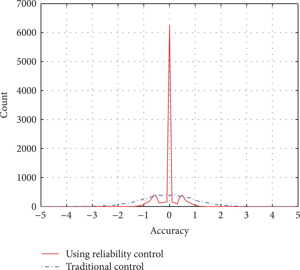
Contrast figure of accuracy distribution in 10,000 times tests.

6. Conclusion

In this paper, a control model of operational reliability is presented. In this model, operational reliability of control system is considered through adding a feedback channel which is used to evaluate the operational reliability and do closed-loop operational reliability control when the manipulator is running. On this basis, a real-time evaluation method of operational reliability is given based on Bayesian method and a regulation strategy of control variable is given as well when the manipulator does not satisfy the reliability requirement of the task.

It has been shown via simulation that the fluctuates of error after the manipulator executing a task significantly reduced, and the success rate of completing a task effectively improves at the same time by using the improved control method described in this paper. Therefore, the reliability of manipulator can be improved by using the control method of operational reliability described in this paper.

Conflict of Interests

The authors declare that there is no conflict of interests regarding the publication of this paper.