Sage Journals: Discover world-class research

Abstract

Time synchronization and localization in underwater environment are challenging due to high propagation delay, time measurement error, and node mobility. Although synchronization and localization depend on each other and have the similar process, they have been usually handled separately. In this paper, we suggest time synchronization and localization based on the semiperiodic property of seawater movement, called SLSMP. Firstly, we analyze error factors in time synchronization and localization and then propose a method to handle those errors. For more accurate synchronization, SLSMP controls the transmission instant by exploiting the pattern of seawater movement and node deployment. Then SLSMP progressively decreases the localization errors by applying the Kalman filter or averaging filter. Finally, INS (inertial navigation system) is adopted to relieve localization error caused by node mobility and error propagation problem. The simulation results show that SLSMP reduces time synchronization error by 2.5 ms and 0.56 ms compared with TSHL and MU-Sync, respectively. Also localization error is lessened by 44.73% compared with the single multilateration.

1. Introduction

Ocean infrastructures like offshore plants have been garnering great attention owing to huge potential benefits of marine resources [1, 2]. Also, necessity of real-time monitoring for marine environment is growing to immediately deal with critical accidents that can be caused by unpredicted events like high temperature of sea water, red tide, oil spill, and so on. According to this trend, many researchers from academic and industrial are studying UWSN (underwater sensor networks) recently. UWSN applications can remotely control marine architectures and monitor marine ecosystem. However, UWSN has some challenges due to the nature of underwater communication channel characterized by error-prone and long propagation delay. In addition, constant movement of underwater sensors has to be accounted for network protocol design. So, it is impossible that we adopt well-refined terrestrial communication mechanisms into the underwater environment directly.

Although time synchronization is crucial for various applications such as localization and low-power sleep scheduling MAC protocols, existing synchronization schemes did not fully consider practical issues, like channel access delay. The delay can be ignored in terrestrial scenario where propagation speeds are extremely high, but not in the water due to the low speed of acoustic signal. Furthermore, contention based MAC protocols like CSMA may cause high channel access delay, resulting in a large gap between the time recorded at a timestamp and the actual transmission instant. As a result, the synchronization error increases because it is based on the accurate time measurement. Last but not least, the node movement also affects the synchronization performance, but it is still remained as a challenge.

Existing localization schemes do not support the localization accuracy requested by recent applications such as a navigation system and a location based routing protocol. Mobility of reference nodes is critical for accurate localization, but it is totally neglected in existing researches. Also, errors in measuring the sending/receiving time, which happen due to constrained hardware capability or signal irregularity, seriously degrade the localization accuracy, but there have been no researches considering them. So, this paper proposes an enhanced time synchronization and localization called SLSMP (synchronization and localization using seawater movement pattern). SLSMP controls the transmission instant by reflecting the fact that node mobility caused by seawater movement like tide and wave follows semiperiodic patterns. Also, SLSMP compensates the sending time recorded at timestamp by removing the channel access delay from timestamp with one more transmission. In addition, the adoption of INS (inertial navigation system) mitigates the influence of node mobility on both synchronization and localization.

The contributions of this paper are listed as follows.

(i)

SLSMP accomplishes time synchronization and localization simultaneously and then it can be applied to many applications and other layers like MAC or network.

(ii)

SLSMP considers node mobility in real-time by using INS and seawater movement pattern.

(iii)

SLSMP deals with the issues of reference inaccuracy and the time measurement error that have not yet been addressed in previous researches on localization. Also, channel access delay, which significantly affects the synchronization, is removed by using application layer timestamp.

The rest of paper is organized as follows. Section 2 introduces previous works related to time synchronization and localization in UWNS. Section 3 defines the error factors in each field and then mathematically and experimentally analyzes how they affect the accuracy of synchronization and localization. Based on the analysis in Section 3, enhanced time synchronization and localization, SLSMP, are proposed in Section 4. Section 5 shows the simulation results, and Section 6 summarizes this paper and suggests future work.

2. Related Work

2.1. Time Synchronization

Time synchronization problem is caused by clock skew and offset. An angular frequency on crystal oscillator is finely drifted by several elements such as temperature, pressure, and voltage, and this variation is called “skew.” Meanwhile offset can be arisen when each sensor node has a different system booting time. TSHL is a time synchronization protocol designed for high propagation and static networks [3]. In TSHL, reference and target node exchange timestamp several times. Then reference node estimates skew and offset through linear regression by exploiting time information acquired during the message exchanges. But it is impractical that they assumed that all nodes are stationary in the underwater environment. To overcome this limitation, MU-Sync provides time synchronization considering mobile scenario [4]. MU-Sync conducts two phase synchronizations. Estimated skew and offset in the first linear regression are utilized to remove propagation delay in received timestamp and the second linear regression carried out with more accurate time information calculates the skew and offset again. MU-Sync accomplished more accurate synchronization than TSHL by improving the accuracy of timestamp. But performance of this protocol is deteriorated when nodes move constantly during the message exchanges because they regard the half of RTT (round trip time) as the propagation delay.

Meanwhile, some synchronization methods try to estimate node mobility so as to improve the accuracy. Synchronization with the Doppler effect is also one of the approaches [5–7]. Those schemes calculate propagation delay just like MU-Sync but they measure frequency shift instead of RTT. Based on relative speed observed in the frequency shift, the reference node establishes several linear equations and then derives skew and offset by solving the simultaneous equation. They, however, unrealistically assumed that Doppler effect is consistently happening during message exchange. Moreover, they did not consider angles between transmitter and receiver, which strongly affect the frequency shift measurements. In addition the performance of those protocols is nondeterministic since relative distance between nodes is changed by their own absolute position which is difficult to know in underwater scenarios. Khandoker et al. [8] have proposed synchronization using node mobility designed by Gauss-Markov model and kinematic model. However, it cannot precisely describe the exact mobility pattern because seawater movement is dynamically changed.

In contrast, SLSMP sophisticatedly measures node mobility in real-time by using INS and semiperiodic properties of seawater movement. Therefore, SLSMP can guarantee the localization accuracy, in spite of node mobility due to seawater movement.

2.2. Localization

Localization for underwater sensor networks has been widely explored, and a number of algorithms have been proposed in [9–13]. However, those protocols are not suitable for underwater networks because they do not consider node mobility that dominantly affects the localization accuracy. Localization considering node mobility was proposed in [14, 15]. Particularly, [15] suggests SLMP which localizes the nodes with two main phases, that is, mobility prediction and localization, based on node mobility patterns demonstrated as a semiperiodic property. All the nodes measure their own trajectory referring to mobility of other nodes at the prediction phase in SLMP. After reference nodes complete the mobility prediction, they broadcast their location and mobility information. If the number of its known reference nodes is equal to or larger than four, a target node conducts localization. Main contribution of the SLMP is that they introduce localization scheme considering node mobility in real-time, but the performance of localization is determined by an accuracy of the mobility prediction. In other word, SLMP cannot guarantee the accurate localization in some cases where mobility prediction is poorly carried out. Particularly, mobility prediction conducted by referring to other nodes’ movement is not appropriate in underwater because spatial correlation is low due to sparse node density. Also, it cannot promptly handle mobility variation since a mechanism detecting and correcting for mobility variation is absent in the SLMP.

Meanwhile, JSL [16] proposes localization scheme joined with time synchronization for underwater sensor networks. Time synchronization is essential for the localization because all localization schemes base on an accurate time measurement. So, JSL alternately conducts synchronization and localization and this approach simultaneously improve both of the accuracies. Furthermore, JSL enhances the localization by adopting IMM filter. IMM filter is an estimation method to trace the state of observing values. The IMM filter predicts mobility patterns of the node by running Kalman and extended Kalman filter in parallel. However, the JSL's performance might be degraded in some cases because a state transition matrix used to model all possible mobility patterns is based on probability. Also, the matrix with only some static values cannot cover dynamically changed mobility patterns. Recently, some researchers have suggested AUV (autonomous underwater vehicle)-aided localization using directional antenna in [17–20]. They improved the localization accuracy because AUV provides relatively high-precision information to the nodes. However, the usage of AUV can restrict the scope of application due to the high cost and difficulty in management. In addition, AUV itself has inaccurate location information because INS error is accumulated during a long-term mission. Consequently, all nodes using the AUV for localization cannot estimate their position correctly.

SLSMP can provide advanced localization by fully considering node mobility without any special equipment like AUV or directional antenna as mentioned above. Also, most previous researches have not considered the mobility of reference nodes and time measurement error frequently happened in underwater scenario. To the best of our knowledge, this is the first research dealing with those practical issues. In Section 3.2, we explain the problems in more detail.

3. Error Analysis

3.1. Time Synchronization

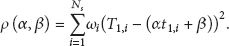
For time synchronization, SLSMP employs linear regression just like TSHL and MU-Sync except for an adoption of weighted mean square error. To improve accuracy of synchronization, we define and analyze error factors on the linear regression in this section. Linear regression is a mathematical tool to infer relationship between two dependent variables [21]. In other words, after establishing a linear equation, $y = a x + b$ , where variables x and y have dependent relationship with each other and regression processing derives a and b that make the sum of squared errors minimum among given data sets. If local time in reference and target node is regarded as x and y, skew and offset are denoted as a and b, respectively, we can synchronize the clock by deriving a and b through linear regression with given timestamps. Let us look at the message exchange process for gathering time information. The reference node writes down its sending time on timestamp and then sends it to target nodes. After receiving the timestamp, target node marks its local time. They acquire time information by repeating this unidirectional message exchange total n times and n has to be large enough to make RMSE (root mean square error) smaller than a predefined acceptable value. We can model time relation between a reference and a target node as follows:

\begin{matrix} T_{i} = α t_{i} + β, \end{matrix}

(1)

where α and β are the skew and offset of the target node and $t_{i}$ and $T_{i}$ are the local time of the reference and the target node, respectively. But random channel access delay caused by contention for channel occupation and propagation delay will be occurred in real message exchanges. Previous studies just focused on the correction of error caused by propagation delay, but this approach is insufficient for accurate time synchronization because channel access delay also affects the accuracy of timestamp as much as propagation delay does in an acoustic channel. Moreover the more nodes contend for channel occupation, the less accurate the delay prediction is. So, the elimination of channel access delay from timestamp is essential. Equation (1) can be rewritten as (2) where propagation and channel access delay in the ith transmission among n time message exchanges are denoted as $e_{p, i}$ , $e_{b, i}$ , respectively, and the sum of both delays is defined as $e_{i}$ :

\begin{matrix} T_{i} = α t_{i} + β + {α e}_{i} . \end{matrix}

(2)

${α e}_{i}$ is substituted by $e_{i}$ for simplicity ( $α ≅ 1$ ) since our concern is only the impact of the $e_{i}$ on linear regression. Then (2) can be rewritten as follows:

\begin{matrix} T_{i} = α t_{i} + β + e_{i} . \end{matrix}

(3)

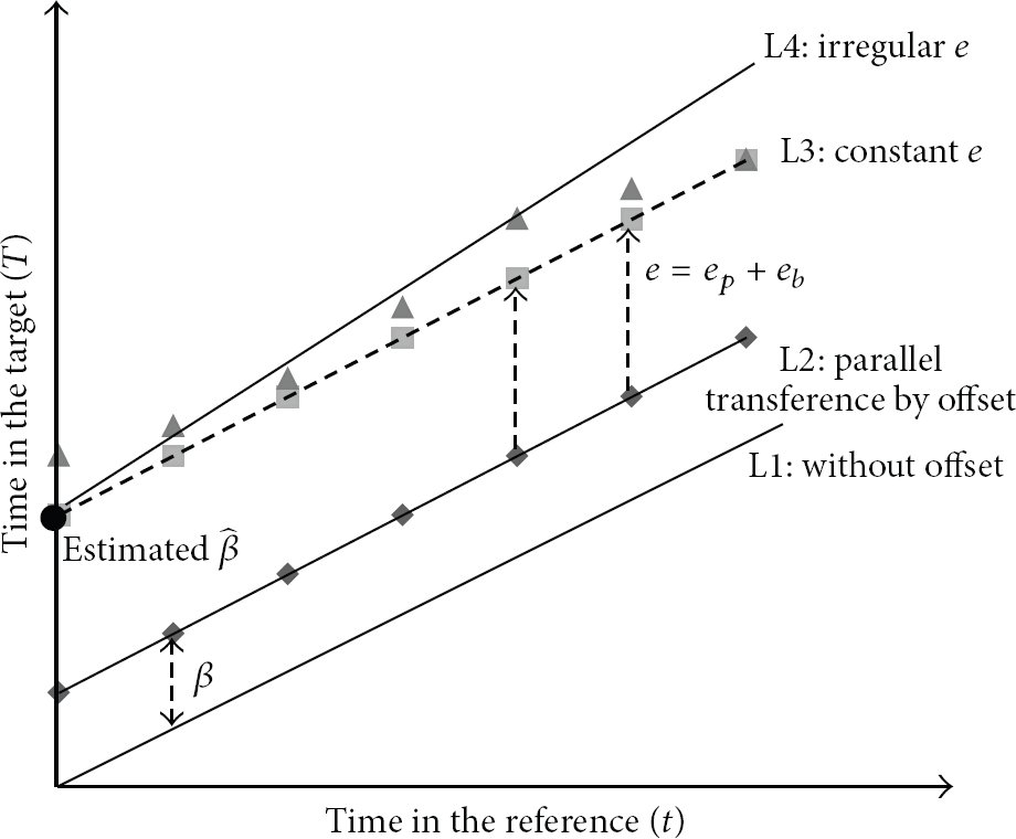
Figure 1 gives us a clue to understand the impact. A time relation between two nodes is formed as L1 and a gradient of L1 is skew. L1 moves to L2 when offset, β, is occurred by different system starting times. We may get linear equation like L4, however, because of $e_{i}$ as mentioned above. The notable thing in Figure 1 is that we can get linear equation having precise skew if all $e_{i}$ is almost same at every message exchange like L3. Strictly speaking, the fundamental error factor in skew estimation is not the propagation and channel access delay themselves but the variation of them at each communication. In previous researches, they intensely focus on how to remove the delays, but it is challenging in underwater where precise skew estimation is quite difficult since unpredictable delays take place at every communication. So our proposed protocol tries to make $e_{i}$ constant rather than removing them from timestamp. That is the novelty of our approach as compared with others.

Figure 1

Illustration of clock drift and impact of measured timestamp on the linear regression.

The sum of squared errors can be represented as follows:

\begin{matrix} ρ (α, β) = \sum_{i = 1}^{n} {(T_{i} - ({α t}_{i} + β))}^{2} . \end{matrix}

(4)

We partially differentiate (4) with α and β, respectively, and then arrange the equation as related to α and β for finding α and β which minimize $ρ (α, β)$ . The expressions are presented as follows:

\begin{matrix} \hat{α} = \frac{n \sum t_{i} T_{i} - \sum t_{i} \sum T_{i}}{n \sum t_{i}^{2} - {(\sum t_{i})}^{2}}, \\ \hat{β} = \frac{\sum t_{i}^{2} \sum T_{i} - \sum t_{i} T_{i} \sum t_{i}}{n \sum t_{i}^{2} - {(\sum t_{i})}^{2}} . \end{matrix}

(5)

Also (3) can be presented as (6) in the same manner:

\begin{matrix} ρ (α, β) = \sum_{i = 1}^{n} {(T_{i} - (α t_{i} + β + e_{i}))}^{2} . \end{matrix}

(6)

If this follows the same process mentioned above, the estimated skew and offset can be calculated, respectively, as follows:

\begin{matrix} \hat{\hat{α}} = \frac{n \sum t_{i} T_{i} - \sum t_{i} \sum T_{i} + \sum t_{i} \sum e_{i} - n \sum t_{i} e_{i}}{n \sum t_{i}^{2} - {(\sum t_{i})}^{2}}, \\ \hat{\hat{β}} = \frac{\sum t_{i}^{2} \sum T_{i} - \sum t_{i} T_{i} \sum t_{i} - \sum e_{i} \sum t_{i}^{2} + \sum t_{i} e_{i} \sum t_{i}}{n \sum t_{i}^{2} - {(\sum t_{i})}^{2}} . \end{matrix}

(7)

The error in skew estimation caused by $e_{i}$ is $\hat{\hat{α}} - \hat{α}$ and the quantity is shown as follows:

\begin{matrix} \hat{\hat{α}} - \hat{α} = \frac{\sum t_{i} \sum e_{i} - n \sum t_{i} e_{i}}{n \sum t_{i}^{2} - {(\sum t_{i})}^{2}} . \end{matrix}

(8)

If we assume that $e_{i}$ at every message exchange is equivalent and reference node sends timestamp in interval I, the numerator in (8) is concisely rewritten as

\begin{matrix} \hat{\hat{α}} - \hat{α} = \frac{n^{2} (n + 1)}{2} e I - \frac{n^{2} (n + 1)}{2} e I = 0 . \end{matrix}

(9)

As you can see in (9), although timestamps include $e_{i}$ , it does not give any impact on skew estimation when they are constant.

Meanwhile, $\hat{\hat{β}} - \hat{β}$ represents the influence of $e_{i}$ on offset estimation and it is calculated as follows:

\begin{matrix} \hat{\hat{β}} - \hat{β} = \frac{\sum t_{i} e_{i} \sum t_{i} - \sum e_{i} \sum t_{i}^{2}}{n \sum t_{i}^{2} - {(\sum t_{i})}^{2}} . \end{matrix}

(10)

The expansion of (10) under the same assumption introduced above can be simplified as follows:

\begin{matrix} \hat{\hat{β}} - \hat{β} = \frac{n^{2} {(n + 1)}^{2}}{4} - \frac{n^{2} (n + 1) (2 n + 1)}{6} . \end{matrix}

(11)

If we do not consider $e_{i}$ on offset estimation, estimated offset results from the sum of original offset and $\hat{\hat{β}} - \hat{β}$ because the equation has always negative values when n is greater than one. As a result, the bigger the average of $e_{i}$ is, the larger the error is in offset estimation.

3.2. Localization

The limitations of the previous localizations are mainly two parts: first, the absence of location updating mechanism on the reference nodes deployed in underwater; second, neglecting time measurement error commonly happened in practice. Their impact on the localization accuracy is specifically explained as follows.

3.2.1. Reference Mobility

All localization algorithms in UWSN estimate node positions in hierarchical manner. Namely, the buoy nodes become the reference node by acquiring location information using GPS. The underwater sensors deployed near the buoy are firstly localized referring to those buoy nodes, and then they also become references. These localization processes will be repeated until all nodes in the network discover their own locations. At the processes, once determined the position, underwater sensors cannot update their position because they do not use any available real-time location system like RTLS or GPS despite the fact that the locations of the sensors are continuously changed. Consequently, the gaps between known and actual current position make localization error.

Let us provide an example to help understand. In Figure 2(a), node E discovers its location as (3, 3, 3) in 3-dimensional space. After that, node E is referred to as reference node for the localization of node F. The location of node E, however, is different from previous localized position, that is, (4, 2, 4) as shown in Figure 2(b). Eventually, node E conducts localization with old information, (3, 3, 3), because it cannot detect or realize the real-time location. The localization error made by the absence of location updating is proportional to the range of movement. In addition, buoy nodes also provide inaccurate location because GPS has location error itself.

Figure 2

Localization errors caused by nonreal-time location of reference nodes.

3.2.2. Errors in Time Measurement

Localization can be categorized into range-based and range-free. In general, the range-based exploiting measured angle or distance between transmitter and receiver is known as more precise localization such as triangulation and multilateration. However, the Range-based schemes cannot guarantee theoretical accuracy when time or distance measurement includes some noises. Some noise factors are briefly summarized as follows.

(i)

Transmission delay: it means the time lag between sending time recorded on a timestamp and actual transmission moment. Commonly, transmitter records sending time at the MAC (medium access control) layer, but the node cannot send the timestamp immediately because some latency is randomly occurred for channel contention. As a result, the transmitter attempts to transfer later than the recorded time.

(ii)

Reception delay: reception delay is the elapsed time from signal detection at a device to interpretation on application layer. Such interrupt handler or radio state transition delay makes reception delay. Unfortunately, sensor nodes cannot appropriately handle since that kind of delay is unpredictable.

(iii)

Time synchronization: as we mention above, frequency of oscillator is finely varied according to external condition like temperature and pressure or by limitation in a process of manufacture. Consequently, that makes some time difference and it is known as skew. Different booting time between each node is also regarded as a main factor in time-sync problem and it is commonly called offset. If each node works on different local times due to skew and offset, localization accuracy will be dramatically dropped. If you want to know about time synchronization in more detail, you can refer to a preceding chapter.

(iv)

Acoustic speed: propagation speed of acoustic is determined according to depth, temperature, and salinity, but almost all studies regard it as constant value, 1500 m/s. This assumption is unpractical since acoustic signal arrives at each reference node with different propagation speeds.

(v)

Refraction of the signal: as mentioned above, propagation speed of acoustic signal is changed according to the state of communication medium and the variation reflects acoustic signals. Consequently, the signal travels along with some curves rather than the straight line. Therefore, ToA (time of arrival) or TDoA (time difference of arrival) which considers distance as the product of propagation speed and reception time difference between receivers cannot estimate accurate distance because they assume propagation path is straight.

Furthermore, multipath padding in shallow water, unpredictable noise in receiver and incidence angle of transmitter can also distort time measurement. To grasp the impact of reference's mobility and time measurement error on multilateration, let us refer to Figure 3. We measured localization errors while increasing the movement boundary from 2 to 4 m and errors in time measurement from 0 to 5 ms. As illustrated in Figure 3, the greater the movement and measurement error is, the more the localization error grows. If acoustic propagation speed and measured time error are denoted by v and delta $Δ t$ , respectively, the distance measurement error can be represented as $Δ t \times v$ ; for example, the error in distance estimation is about 1.5 m with 1 ms time measurement error.

Figure 3

Influence of errors in time measurement and node mobility on localization accuracy.

Although time measurement error and unreliability of the reference position severely affect localization accuracy as described above, previous researches do not consider those error factors into localization at all. In addition, most of them just focus on insignificant topics such as how to reduce the number of required reference or message overhead rather than improvement of localization accuracy. Therefore, we propose enhanced and practical UWSN localization while considering the error factors using INS and filter theories in the next section.

4. Proposed Method

4.1. System Description

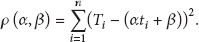
The target aquatic environment of our protocol is offshore with a depth of less than 400 m. In this application, we assume that transmission range is within 100 m even though the currently developed transmitter module can send a packet further than our assumption. This is due to the fact that multihop communication is more reliable than direct communication because multipath fading dominantly drops the packet delivery ratio in the offshore [22]. SLSMP is organized as shown in Figure 4. The reference nodes are attached to buoys and can get the global time from GPS and GPS provides real-time location to the references. We assume that sensor nodes deployed in underwater are equipped with tiny gyro and acceleration sensors thanks to MEMS (microelectro mechanical systems) technology. Those sensors act as INS (inertial navigation system) to trace the node's trajectories in real time.

Figure 4

System description.

Node deployment in underwater is another challenge and how to deploy the sensors is mainly determined by application's features. However, in general scenario, underwater researches assume that each node is fastening to seabed or ocean infrastructures with a wire or an anchor [23]. Therefore our target system follows the manner and then node mobility is just allowed within certain boundary. Also, according to the ocean hydrodynamic and real experiments, ocean currents apply periodic force to floating objects [24, 25]. In other words, nodes move around not randomly but semiperiodically. Based on this knowledge, we insist that all nodes have semiperiodical mobility pattern.

4.2. Protocol Overview

In this section, we briefly describe SLSMP protocol. SLSMP consists of three phases, namely, SP (sending point) selection based on trajectory tracking, message exchange, and time synchronization/localization. Most of all, underwater sensors record their semiperiodical mobility pattern using INS for some interval and then decide SP. SP is the only site where the target node sends a timestamp. This effort makes the target node stationary even though the node is constantly moving actually. Consequently, error caused by node mobility in synchronization/localization is markedly relieved. It will be specifically explained later. To extract the SP from the recorded trajectories, the sensor evenly divides the movement area into several small cubes and examines how many times it is located at each cube during the trajectory tracking phase. The highest hit ratio means that the node has arrived at the location frequently and it will reach the cube in the future periodically. If the node founds several points with the same hit ratio, a cube with smallest moving speed of the node is preferentially selected as SP. This is due to the fact that a node maybe sends a timestamp in the near SP instead of correct SP because the transmission can be delayed by the MAC access delay and the node moves to other places during that time. If node's moving speed per unit time is low, however, the transmission point is almost the same with the SP since the node rarely moves in the area. After selection of the SP, the target node monitors their location in real-time and sends timestamp only when it is located at SP. Upon receiving a packet, the references record reception time and receiving position and reply with a timestamp including the recorded information. After this message is exchanged several times, SLSMP completes time synchronization and localization with linear regression and filtering, respectively. In the following sections, we will describe the details of the algorithm.

4.3. Time Synchronization

From Section 3, we know that propagation and channel access delay affect the accuracy of time synchronization based on linear regression. Also, we can improve the synchronization accuracy by keeping the values as a constant at all message exchanges. The ultimate goal of SLSMP stems from these observations; thus SLSMP will try to make equivalent $e_{i}$ at every message exchange to form the time relation like L3 in Figure 1. In addition, based on the estimated skew, offset can be derived by calculating RTT. In order to achieve our design goal, we introduce two methods: first, elimination of the channel access delays from timestamps using additional one more transmission; second, maintaining the $e_{p, i}$ as the same value for every message exchange. To the best of our knowledge, this is the first research that utilizes node mobility pattern for time synchronization.

Although timestamp can be recorded at all layers except for the PHY layer, writing a transmitting time at lower layers is more desirable since unpredictable delay might be happened during packet delivery from upper to lower layers. Unfortunately, current MAC timestamp mechanisms cannot deal with time difference between the recorded transmitting time on timestamp and the real transmission instant due to the channel access delay as shown in Figure 5(a). To remove this gap, we propose application layer timestamp. 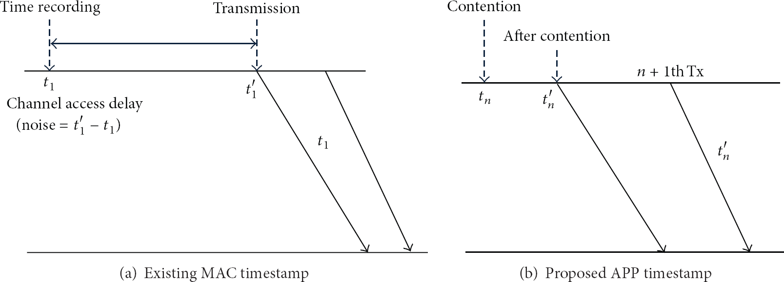In SLSMP, the ( $n + 1$ )th timestamp includes the nth transmission time as illustrated in Figure 5(b). After random channel access delay, a sensor node writes the instant of transmission on memory and then delivers the recorded time on the next transmission. A target node can acquire the nth timestamp not including channel access delay in the ( $n + 1$ )th timestamp. So sensor node can utilize a precise timestamp without channel access delay even if a number of nodes are contending for a channel. Although SLSMP requires additional transmission, it is trivial overhead in the message exchange process where numerous transmissions and receptions occurred.

Figure 5

Influence of channel access delay on timestamp.

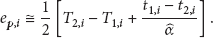
Meanwhile, to maintain the sum of channel access and propagation delays $e_{i}$ as constant, SLSMP exploits the feature of seawater movement and node deployment. As mentioned above, a target node begins message exchange by broadcasting its timestamp when it is located at SP. When a target node broadcasts the ith timestamp, it contains the ( $i - 1$ )th transmission time $T_{1, i - 1}$ and propagation delay $e_{p, i - 1}$ . A way of how to calculate the propagation delay is explained later.

If a target node broadcast timestamp, multiple references will receive the packet, so a reference among them is randomly selected for time synchronization. Upon receiving a packet, the selected reference node records the target's timestamp $T_{1, i - 1}$ , the packet reception time $t_{1, i}$ , and their receiving location, $p_{i} = (x_{i}, y_{i}, z_{i})$ , respectively. After that, the reference node sends $p_{i}$ and their replying time $t_{2, i}$ to the target node. Other nonselected reference nodes also send their reception time and position for calculation of TDoA used in localization. Upon receiving a packet from the reference, the target node checks reception time $T_{2, i}$ and calculates propagation delay as follows:

\begin{matrix} e_{p, i} ≅ \frac{1}{2} [T_{2, i} - T_{1, i} + \frac{t_{1, i} - t_{2, i}}{\hat{α}}] . \end{matrix}

(12)

The message exchange process is depicted in Figure 6. After finishing the message exchange phase, the selected reference node calculates its average receiving locations, $p_{m} = (\bar{x}, \bar{y}, \bar{z})$ . In addition, the selected reference node sets up an equation for a method of weighted least squares as follows:

\begin{matrix} ρ (α, β) = \sum_{i = 1}^{N_{s}} ω_{i} {(T_{1, i} - (α t_{1, i} + β))}^{2} . \end{matrix}

(13)

If the speed of propagation acoustic channel is v, the weight, $ω_{i}$ , is represented as follows:

\begin{matrix} ω_{i} = 1 - \frac{D_{i, m}}{v}, \end{matrix}

(14)

where $D_{a, b}$ is distance between points a and b.

Figure 6

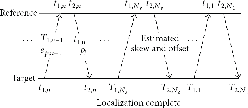
Message exchange between reference and target nodes.

The ultimate purpose of weights is to minimize the skew estimation error caused by variation of the reference's receiving locations at each message exchange. Weights multiplied by the squared errors adjust the impact of errors on skew estimation. In other words, if the receiving location is far from $P_{m}$ , the weight is decreased to reduce the impact of the error; otherwise the weight increases according to (14). Finally, we can derive skew, α, satisfying (15) using the partial derivative:

\begin{matrix} ρ (\hat{α}, \hat{β}) = \arg \min [α, β] . \end{matrix}

(15)

After estimating the skew, we calculate the offset by utilizing the estimated skew. The $e_{i}$ consist of propagation and channel access delay, but channel access delay, $e_{b, i}$ , can be ignored with application timestamp suggested in Section 4.3. Therefore we make an equation by referring to (2) as follows:

\begin{matrix} β_{i} = T_{1, i} - α (t_{1, i} + e_{p, i}), \end{matrix}

(16)

where $β_{i}$ is offset calculated in the $i + 1$ th message exchange. Ultimately, the offset between two nodes is estimated as follows:

\begin{matrix} \hat{β} = \frac{1}{k} \sum_{i = 1}^{N_{s}} β_{i} . \end{matrix}

(17)

4.4. Localization

Meanwhile, after selection of the SP, target node monitors their location in real-time and sends a timestamp to references only when it is in the SP for localization. Upon receiving a timestamp, the references record the reception point and time and reply to the target by transferring the recording information. If the number of references is greater than or equal to four, the target discovers its location by referring to them. SLSMP adopts multilateration already which introduced many previous researches. Before discussing our localization protocol, let us introduce multilateration briefly. When target node K and references A, B, C, and D are deployed in the network, we denote the position of k and a certain target node as ( $x, y, z$ ) and ( $x_{R}$ , $y_{R}$ , $z_{R}$ ), respectively ( $R \in {A, B, C, D}$ ). The corresponding ToA (time of arrival) at each reference is given by the following equations:

\begin{matrix} T_{R} = \frac{1}{v} \sqrt{{(x - x_{R})}^{2} + {(y - y_{R})}^{2} + {(z - z_{R})}^{2}}, \end{matrix}

(18)

where v is propagation speed of acoustic signal. If the node A is selected as reference point, the calculation of TDoA $τ_{A}$ between A and K is calculated by

\begin{matrix} τ_{A} = \frac{1}{v} \sqrt{x^{2} + y^{2} + z^{2}} . \end{matrix}

(19)

The calculation of TDoA $τ_{R}$ between certain reference node R and A is calculated by

\begin{array}{l} τ_{R} = T_{R} - T_{A} \\ = \frac{1}{v} (\sqrt{{(x - x_{R})}^{2} + {(y - y_{R})}^{2} + {(z - z_{R})}^{2}} \\ - \sqrt{x^{2} + y^{2} + z^{2}}) + e_{m} . \end{array}

(20)

In (20), the $e_{m}$ is time measurement error happened in actual communication. Finding a location of target (x, y, z) using (20) is not to get unique solution but to minimize the sum of squared errors, that is, optimization problem. So, in this paper, the Levenberg-Marquardt (LM) algorithm was adopted to find an optimization solution in nonlinear localization system. However, the estimated location still has some error due to the inaccuracy of the references and time measurement. Therefore, some compensation scheme is required to improve the localization performance.

Accurate location estimation with only one localization process is very difficult in harsh underwater environment containing many unpredictable measurement errors and node mobility. Instead, we can get the more accurate location by conducting multiple localization processes. In other words, localization accuracy will be gradually improved by repetitive estimation and correction operations progressing until the accuracy is stable. Therefore, SLSMP performs location estimation a total of n times only when the target is in predefined area SP. The ith estimated location of target node through multilateration is denoted by $P_{m, i}$ . Then the $P_{m, i}$ becomes input to filters for iterative data processing. Meanwhile, considered filters for error correction in this paper are the Kalman filter and averaging filter. They are explained in more detail as below.

4.4.1. Kalman Filter

The Kalman filter widely used in many fields is a recursive data processing algorithm to estimate unknown variables containing random errors [26]. The unknown values mean target location represented by (x, y, z) in underwater space. It is already introduced and utilized in some underwater localization like JSL [16], the representative localization protocol exploiting the Kalman filter. The JSL uses IMM filter, a mixture of Kalman filter and EKF (extended Kalman filter), to estimate the target location and approximate the node trajectory with state transition matrix. However, it is impossible that the state transition matrix precisely describes all possible node mobility patterns due to their natures described by probabilistic and static. As a result, localization performance might get worse considerably. Also, the EKF which smoothly linearizes nonlinear system has a possibility of divergence when initial estimation is wrong or system design is inappropriate. In contrast to the JSL, the proposed method is independent of all possible mobility patterns on the use of the Kalman filter by sending the timestamp only at the specific areas, SP. In other words, we make the system linearly to avoid impractical modeling. State variables V, state transition matrix A, and matrix H representing change of the states are determined as

\begin{matrix} V = (\begin{pmatrix} x \\ y \\ z \end{pmatrix}), H = (\begin{pmatrix} 1 & 0 & 0 \\ 0 & 1 & 0 \\ 0 & 0 & 1 \end{pmatrix}), A = (\begin{pmatrix} 1 & 0 & 0 \\ 0 & 1 & 0 \\ 0 & 0 & 1 \end{pmatrix}) . \end{matrix}

(21)

Also initial parameters adjusting Kalman gain is denoted as

\begin{matrix} Q = (\begin{pmatrix} 0 & 0 & 0 \end{pmatrix}), R = (\begin{pmatrix} 4 & 0 & 0 \\ 0 & 4 & 0 \\ 0 & 0 & 4 \end{pmatrix}) . \end{matrix}

(22)

Estimated location by the ith iteration is denoted as $P_{k, i}$ and final estimation of the node is completed through $N_{l}$ times of iteration.

4.4.2. Averaging Filter

Estimation accuracy of the Kalman filter is influenced by the reliability of the system modeling. Moreover, in cases where distribution of the measured locations or measured time errors do not follow a normal distribution, the filter performance cannot be guaranteed because the basic assumption of the Kalman filter is that the errors follow a normal distribution.

Consequently, localization using the Kalman filter has some challenge in underwater where the time measurement errors arise nondeterministically. Accordingly, we consider the potential of the averaging filter which does not require system modeling in contrast to the Kalman filter [27]. Intuitively speaking, the averaging filter estimates current state as the average of the observed data. The measured locations $P_{m, i}$ are distributed around the SP because every localization of the target is carried out only in the SP. Thus, the average of $P_{m, i}$ can improve the localization accuracy by countervailing the estimated location errors. Estimated location $P_{a, i}$ through the ith iteration of the averaging filter can be represented by recursive equation as follows:

\begin{matrix} P_{a, i} = \frac{i - 1}{i} P_{a, i - 1} + \frac{1}{i} P_{a, i} (P_{a, 0} = P_{m, 1}) . \end{matrix}

(23)

The Kalman and averaging filters are the same in terms of iterative data processing to estimate the state. The crucial difference between two filters is that the Kalman filter dynamically adapts weight to measured values at every estimation phase based on the difference between prediction and actual measurement while the averaging filter just assigns the same weight to all measured values as illustrated in (23). Therefore, the performances of Kalman filter known as optimal recursive data processing algorithm is similar to or lower than the averaging filter according to system modeling reliability and the distribution of measured locations.

Finally, the target nodes discover SP through a total of $N_{l}$ times multilateration and error correction with filters as described above. The process of each filter for localization is described in Figure 7. After that, the target nodes update their position in real time using INS to provide the newest information to other target nodes. As a result, the localization accuracy will be considerably increased by removing the impact of reference mobility in localization process.

Figure 7

The work flow of the each filter for localization.

5. Simulation

5.1. Mobility Modeling

Tidal areas are determined by the strength of tidal currents and the shallowness. The interaction of tidal currents and the sharp of bottom make residual currents. Thus a flow field in tidal areas is dominantly created by a tidal and a residual current field. We modeled the flow field as follows. The kinematic model in [15] is one of the general solutions. This model roughly approximates the node mobility. According to the model, speed of a node in X and Y directions is represented as

\begin{matrix} V_{x} = k_{1} λ \sin (k_{2} x) \cos (k_{3} y) + k_{1} λ \cos (2 k_{1} t) + k_{4}, \\ V_{y} = - λ v \cos (k_{2} x) \sin (k_{3} y) + k_{5}, \end{matrix}

(24)

where $k_{1}$ , $k_{2}$ , $k_{3}$ , $k_{4}$ , $k_{5}$ , λ, and v are probability variables related to the environmental factors. Although some papers adopt this model to simulate their protocols, we cannot directly use them in our simulation. This is the due to the fact that underwater node has some movement boundaries by a loop in our assumption. We measure trajectory of a node in x direction based on (24) by utilizing the integral and the result is depicted in Figure 8(a). The node position is periodically changed forming sine curve but one notable thing is that the node is gradually drifted to x direction. Consequently, if some boundary cannot be established, the node is away from mission area and eventually loses its purpose. As a result, this model cannot fully describe node mobility pattern because feature of deployment is ignored. Figure 8(b) shows measurement of the node trajectory with the same parameters except for boundary setting. As seen in the figure, the node trajectory has semiperiodical properties within some boundary. This is more practical model considering node deployment. In addition, the node periodically reaches the same location pointed with circles in the figure, that is, 20 m in x direction. This result supports our assumption that the node periodically arrives at some area represented by SP in this paper.

Figure 8

A node trajectory (a) without boundary restriction and (b) with boundary.

Then we simplify and approximate the model as elliptical orbit in an $x - y$ plane. The main contribution of this modeling is explained as two parts. First, according to the simulation results, the boundary width is rapidly changed with a small growth of $k_{1}$ and λ in (24). So, the model cannot show the gradual change of errors according to the growth of boundary width. Second, the kinematic model is subject to node speed rather than position. Therefore, the model cannot show impact of node movement in synchronization and localization intuitively. Our node mobility model is represented as follows:

\begin{matrix} \frac{{(x - x^{'})}^{2}}{τ^{2}} + \frac{{(y - y^{'})}^{2}}{μ^{2}} = 1, \end{matrix}

(25)

where τ and μ are subject to the normal distribution with τ and μ as the mean and $0.1 τ$ and $0.1 μ$ as the standard deviation respectably and $x^{'}$ , $y^{'}$ are initial location of the node. Our model is more simple and practical while having similar semiperiodical properties with the kinematic model. The node deployment and mobility modeling is described in Figure 9.

Figure 9

Node deployment and mobility design.

Also, the simulation parameters are summarized in Table 1. The network size is $400 \times 400 \times 400 m^{3}$ . This is because we assume that the maximum transmission range is 100 m and maximum hop count is three. According to the datasheet for Berkeley motes [28], the upper bound of skew is 40 ppm and previous synchronization literatures commonly follow that. The offset of 5 seconds is assumed between a reference and a target node at the beginning. A GPS has some location errors ranging from 0.5 m to 3 m in general and they can be increased or decreased depending on the used technology, weather condition, seawater movement, and so forth. Here, we decide the GPS error as 1.7 m without loss of generality.

Table 1

Simulation parameters.

Simulation parameter	Value
Network size	$400 \times 400 \times 400$ (m³)
Skew, α	40 (ppm)
Offset, β	5 (s)
# of node	125
GPS error	1.7 m
# of simulation	100 times
τ	2 m
μ	2 m
Topology	Grid

5.2. Time Synchronization

To evaluate SLSMP, well-known schemes, TSHL and MU-Sync using linear regression like our protocol, are selected as the comparisons. Firstly, we observed the errors on skew estimation as increasing the number of transmission and Figure 10 represents the simulation results. In this simulation, MU-Sync and TSHL need to transmit the timestamp fifty times for convergence of the accuracy of skew estimation while the number of required packets in SLSMP is just twenty. This is due to the fact that the accuracy of skew estimation is low when nodes move constantly during message exchange. This situation occupies a large part in a small amount of message exchange in comparisons. On the other hand, SLSMP prevents that problem by keeping the distance between two nodes with adjustment of transmission location and weight based linear regression. Therefore SLSMP conducts synchronization using less transmission. One notable thing is that SLSMP's estimation error looks like almost zero in the figure, but it is because the error is very small relatively as compared with others. In SLSMP, the error in case of four times of message transmissions is actually 0.023 ms and the error decreases as to the number of message exchange increases like other protocols.

Figure 10

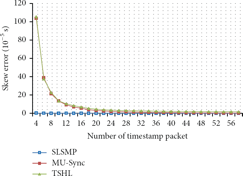
Effect of the number of timestamp on skew estimation.

Figure 11 shows the impact of channel access delay on offset estimation. As in the analysis in Section 3, errors on offset estimation are proportional to channel access delay in the compared protocols. The accuracy on offset estimation in SLSMP, however, is not affected by channel access delay because the delay is removed from timestamps. The reason why MU-Sync more accurately estimates offset than TSHL is that MU-Sync eliminates some part of channel access delay from timestamps when propagation delays are removed. From the simulation result, we can say that the SMP-Sync provides more reliable timestamps no matter how many active nodes contend for a channel occupation.

Figure 11

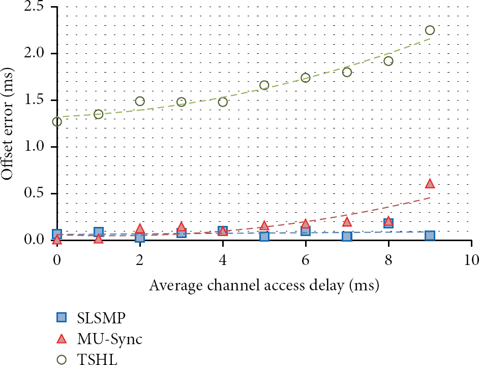
Effect of channel access delay on offset estimation.

Figure 12 shows that the error in time estimation since execution of time synchronization where average channel access delay is assumed as 10 ms. SLSMP shows better time estimation as compared with others thanks to the more precise skew and offset estimation. The accurate time estimation has advantages in terms of not only provision of accurate time but also long time synchronization interval leading to saving the energy.

Figure 12

The error in time estimation since synchronization.

Finally, we evaluated the accuracy of skew estimation in the case that each node has some randomness in their mobility. Although seawater flow cannot be abruptly changed within certain area in an instant, unpredictable external force, for example, a school of fish or fishing craft's activities, can affect the node's trajectory. Nevertheless, the sensor node still detects a proximity to the SP, because INS traces the real time location of the node. However, it takes much time for a node to reach the SP since the previous transmission. Naturally, time for synchronization will be increased and they will bring about the accumulated error in the trajectory tracking. In other words, as time goes on, the error makes a certain difference between the original SP and the estimated SP. To grasp the impact of the tracking error on SLSMP, we observed the error in skew estimation according to the tracking errors following probability distribution, N~ $(μ, 1)$ , and the mean, μ, was varied from 0 to 3.0 m. As you can see in Figure 13, the estimating errors rarely grow although the tracking error increases. This is because node recognizes wrong position as the original TP and keeps sending timestamp at the wrong position. As a result, the transmission location was still fixed at the wrong point. From the simulation result, our method is capable of handling non-periodic mobility pattern by exploiting the characteristic of node deployment and sensor fusion technology, that is, INS.

Figure 13

Effect of INS error on skew estimation.

5.3. Localization

One of the main contributions is that SLSMP considerably improves localization accuracy as well as time synchronization. In this simulation, we choose a single multilateration without the INS as a comparison. In addition, we do not take account of some cases where a target node cannot conduct localization due to the relative location from the references because the ultimate goal of the simulations is only to evaluate localization accuracy. That problem is specifically described in [13]. We denote the SLSMP with the averaging filter as SLSMP-A and the Kalman filter as SLSMP-K, respectively.

It is true that the more the number of iteration is, the better the accuracy has in location estimation using filters. However, the proposed method must control the number of messages exchanged because excessive number of messages cause severe energy consumption. So, we must find out the optimal number of message exchanges that is enough to guarantee convergence of the localization accuracy. Figure 14 shows localization errors according to the number of message exchanges where the error in time measurement is 1 ms, and $α$ and β are 2 m, respectively. Localization error gradually goes down with the increase of the number of message exchanges in SLSMP as illustrated by Figure 14. In the comparison between the two filters, the Kalman filter shows somewhat high accuracy, but the difference is trivial. This is due to the fact that system modeling and parameters adjusting Kalman gain heavily affect the estimation accuracy. Also, this is consistent with our explanation. Meanwhile, SLSMP decides the number of message exchanges as twenty based on the simulation result.

Figure 14

The localization error according to the number of iteration.

Figure 15 describes the effect of time measurement error on localization. In this simulation, the error is generated by the product of probability variable, z, following normal distribution and time error $Δ t$ . As mentioned above, among a lot of factors affecting the error, the variation of channel access delay and acoustic propagation delay is one of the most important ones. However, we consider only the latter in our simulation because the channel access delay has been already removed by adopting the application layer timestamp. The acoustic velocity c is determined by the following equation:

\begin{array}{l} c = 1449.2 + 0.016 z + 4.6 T - 0.055 T^{2} + 0.00029 T^{3} \\ + (1.34 - 0.01 T) (S - 35) [m / s], \end{array}

(26)

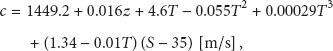
where T, S, and z are temperature, depth, and salinity, respectively. In short-haul communication, that is, within 100 m transmission range, T and z are always same in all areas in our network. If we assume that T and z are fixed and temperature is 35°C, the time measurement error is about 2 ms with 100 m commutation range in a grid topology. So, we observe the localization error while varying $Δ t$ from 0 to 2 ms. In the figure, the localization accuracy in all protocols is declined with the increase of the time errors. As you can see from the gradient of each protocol, however, SLSMP is less affected by the error as compared with the only multilateration. This is due to the fact that localization errors are corrected by the filters. Actually, SLSMP reduces localization error by 2.8 m as compared to the multilateration scheme when the time measurement error, $Δ t$ , is 2 ms. Meanwhile, the difference is gradually lessened as $Δ t$ becomes smaller, and the multilateration method gives the higher performance than SLSMP while $Δ t$ is less than 0.7 ms. This is because multilateration is enough to accurate localization itself in small time measurement error, whereas SLSMP might be affected by some outliers during interactive data processing.

Figure 15

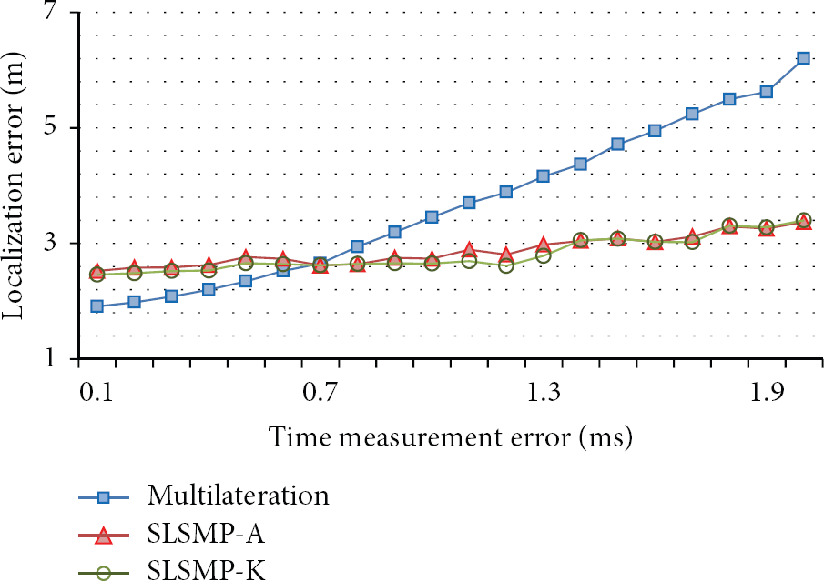
Effect of errors in time measurement on localization.

One of the advantages of SLSMP is durable against node mobility. To prove this, we observe the localization errors while changing τ from 2 to 8 m. As shown in Figure 16, the more the node mobility grows, the bigger the localization error is in all methods. However, growth rate of the error in SLSMP is relatively low than the other by using fresh location information given by INS. Actually, SLSMP reduces the localization error by 3.4 m when mobility range τ is 8 m. It means that the INS is outstanding equipment in underwater localization.

Figure 16

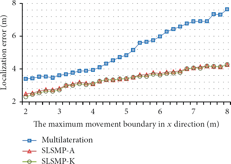
Effect of node mobility on localization.

As the localization is progressed, localization error will be accumulated. Figure 17 shows the mean of localization error from randomly chosen 16 nodes according to the hop count. As illustrated in the figure, although the localization accuracy of all methods is gradually reduced with growth of hop-distance, SLSMP shows a similar localization error at each hop distance. This is due to the fact that the location accuracy of the reference is affected by accumulated error and node mobility in the comparison. In contrast, only accumulated error affects the reference accuracy thanks to the INS relieving an impact of node mobility. From the simulation result, we can say that SLSMP is obviously practical in the deep sea where normally multihop communication is used in the networks.

Figure 17

Impact of accumulated errors according to the hop distance.

Finally, we analyze the impact of the INS accuracy on the localization. So far, SLSMP assumes that the INS provides accurately updated location to the nodes and consequently target nodes are able to send a timestamp only when they reach the exact SP. However, many industrial experts address the problem of INS error and it can rapidly be increased by an unexpected tide. Therefore, the target will send a timestamp around SP rather than correct SP due to the misunderstanding about its current location as mentioned in time synchronization simulation. In addition, the location updating is not precise anymore by the INS error and it makes the reference location inaccurate. Although the INS error problem was addressed by experts recently, the exact values have not been reported so far because the error is not predictable and controllable. In this simulation, localization error was observed while varying the INS error from 0 to 0.5 m. Figure 18 shows difference of localization error in the absence and the presence of INS errors. As shown in the figure, the localization error cannot be notably increased, though the INS error is growing. This is due to the fact that the INS error is counterbalanced on the multiple reference nodes according to size or direction of the errors. From the result, it is obvious that node mobility and time measurement error dominantly affect the localization process rather than INS error.

Figure 18

Effect of INS error on localization.

6. Conclusion

We proposed enhanced time synchronization and localization, named SLSMP, using features of seawater movement and sensor deployment. We define error factors affecting the accuracy of synchronization and localization with mathematical and experimental analysis. The adjustment of transmission instant and weighted least squares regression relieves skew estimation error caused by variation of propagation delay. Moreover, SLSMP provides more practical and accurate synchronization because the unpredictable channel access is removed by applying the application layer timestamp. Furthermore, localization accuracy is considerably improved with knowledge about sensor deployment, INS and filter technique. One interesting fact is that the Kalman filter and averaging filter have similar performance. The simulation results show that SLSMP outperforms the previous well-known time synchronization protocols, TSHL and MU-Sync, in terms of the time accuracy and SLSMP also shows better performance in practical network environment containing time measurement errors and unreality of reference node as compared with a single multilateration.

In the future, we plan to enhance our work to localize mobile objects like AUV (autonomous unmanned vehicle). To do so, we will investigate the prediction algorithm for the mobile patterns and devise how to combine SLSMP with them.

Footnotes

Acknowledgment

This work was supported by the Industrial Strategic Technology Development Program (no. 10043907) funded by the Ministry of Knowledge Economy (MKE, Korea).

References

Kheirabadi

M. T.

Mohamad

M. M.

Greedy routing in underwater acoustic sensor networks: a survey

International Journal of Distributed Sensor Networks 2013 2013 21

701834

10.1155/2013/701834

Heidemann

Wills

Syed

Research challenges and applications for underwater sensor networking

Proceedings of the IEEE Wireless Communications and Networking Conference (WCNC '06)

April 2006

Las Vegas, Nev, USA

228 235

2-s2.0-34250365027

10.1109/WCNC.2006.1683469

Syed

A. A.

Heidemann

Time synchronization for high latency acoustic networks

Proceedings of the 25th IEEE International Conference on Computer Communications (INFOCOM '06)

April 2006

Barcelona, Spain

1 12

2-s2.0-39049102879

10.1109/INFOCOM.2006.161

Chirdchoo

Soh

W.-S.

Chua

K. C.

MU-Sync: a time synchronization protocol for underwater mobile networks

Proceedings of the 3rd ACM International Workshop on Underwater Networks (WuWNet '08)

September 2008

San Francisco, Calif, USA

35 42

2-s2.0-70549108000

10.1145/1410107.1410115

Mirza

Schurgers

D-sync: doppler-based time synchronization for mobile underwater sensor networks

Proceedings of the 5th ACM International Workshop on Underwater Networks (WUWNet '10)

September 2010

Woods Hole, Mass, USA

2-s2.0-78650139691

10.1145/1868812.1868815

Liu

Wang

Peng

Zuba

Cui

J.-H.

Zhou

TSMU: a time synchronization scheme for mobile underwater sensor networks

Proceedings of the IEEE Global Telecommunications Conference (GLOBECOM '11)

December 2011

Houston, Tex, USA

1 6

2-s2.0-84857222301

10.1109/GLOCOM.2011.6134447

Liu

Wang

Zuba

Peng

Cui

Zhou

DA-Sync: a doppler assisted time synchronization scheme for mobile underwater sensor networks

IEEE Transactions on Mobile Computing 2013 1

10.1109/TMC.2013.13

Khandoker

T. I.

Fang

Huang

Sreeram

A robust time synchronization approach for underwater networks with inconsistent timestamps

Proceedings of the International Symposium on Communications and Information Technologies (ISCIT '12)

October 2012

Gold Coast, Australia

1086 1091

10.1109/ISCIT.2012.6380854

Zhou

Cui

J.-H.

Zhou

Efficient localization for large-scale underwater sensor networks

Ad Hoc Networks 2010 8 3 267 279

2-s2.0-72949095657

10.1016/j.adhoc.2009.08.005

10.

Garcia

J.-E.

Ad hoc positioning for sensors in underwater acoustic networks

Proceedings of the MTS/IEEE Techno-Ocean (OCEANS '04)

November 2004

Kobe, Japan

2338 2340

2-s2.0-19544381324

10.1109/OCEANS.2004.1406519

11.

Zhang

Cheng

A distributed protocol for multi-hop underwater robot positioning

Proceedings of the IEEE International Conference on Robotics and Biomimetics (ROBIO '04)

August 2004

Shenyang, China

480 484

2-s2.0-28344434189

10.1109/ROBIO.2004.1521826

12.

Cheng

Shu

Liang

D. H.-C.

Silent positioning in underwater acoustic sensor networks

IEEE Transactions on Vehicular Technology 2008 57 3 1756 1766

2-s2.0-44849108659

10.1109/TVT.2007.912142

13.

Cheng

Teymorian

A. Y.

Cheng

Underwater localization in sparse 3D acoustic sensor networks

Proceedings of the 27th IEEE Conference on Communications (INFOCOM '08)

April 2008

Phoenix, Ariz, USA

236 240

2-s2.0-51349120278

10.1109/INFOCOM.2007.56

14.

Mirza

Schurgers

Energy-efficient ranging for post-facto self-localization in mobile underwater networks

IEEE Journal on Selected Areas in Communications 2008 26 9 1697 1707

2-s2.0-57049173136

10.1109/JSAC.2008.081209

15.

Zhou

Peng

Cui

J.-H.

Shi

Bagtzoglou

Scalable localization with mobility prediction for underwater sensor networks

IEEE Transactions on Mobile Computing 2011 10 3 335 348

2-s2.0-78751605771

10.1109/TMC.2010.158

16.

Jun

Zhaohui

Zuba

Zheng

JSL: joint time synchronization and localization design with stratification compensation in mobile underwater sensor networks

Proceedings of the 9th Annual IEEE Communications Society Conference on Sensor, Mesh and Ad Hoc Communications and Networks (SECON '12)

June 2012

Seoul, Republic of Korea

317 325

10.1109/SECON.2012.6275793

17.

Erol

Vieira

L. F. M.

Gerla

AUV-aided localization for underwater sensor networks

Proceedings of the International Conference on Wireless Algorithms, Systems and Applications (WASA '07)

August 2007

Chicago, Ill, USA

44 54

2-s2.0-46849119215

10.1109/WASA.2007.143

18.

Luo

Guo

Dong

Hong

Zhao

LDB: localization with directional beacons for sparse 3D underwater acoustic sensor networks

Journal of Networks 2010 5 1 28 38

2-s2.0-77950869742

10.4304/jnw.5.1.28-38

19.

Waldmeyer

Tan

H.-P.

Seah

W. K. G.

Multi-stage AUV-aided localization for underwater wireless sensor networks

Proceedings of the IEEE Workshops of International Conference on Advanced Information Networking and Applications (WAINA '11)

March 2011

Singapore

908 913

2-s2.0-79957570769

10.1109/WAINA.2011.90

20.

Erol-Kantarci

Mouftah

H. T.

Oktug

Localization techniques for underwater acoustic sensor networks

IEEE Communications Magazine 2010 48 12 152 158

2-s2.0-78650880584

10.1109/MCOM.2010.5673086

21.

Montgomery

D. C.

Peck

E. A.

Vining

G. G.

Introduction to Linear Regression Analysis 2011 4th

Hoboken, NJ, USA

John Wiley & Sons

Wiley Series in Probability and Statistics

22.

Stojanovic

Preisig

Underwater acoustic communication channels: propagation models and statistical characterization

IEEE Communications Magazine 2009 47 1 84 89

10.1109/MCOM.2009.4752682

23.

Akyildiz

I. F.

Pompili

Melodia

Underwater acoustic sensor networks: research challenges

Ad Hoc Networks 2005 3 3 257 279

2-s2.0-13944252629

10.1016/j.adhoc.2005.01.004

24.

Novikov

Bagtzoglou

A. C.

Hydrodynamic model of the lower Hudson river estuarine system and its application for water quality management

Water Resources Management 2006 20 2 257 276

2-s2.0-33645093945

10.1007/s11269-006-0320-9

25.

Bagtzoglou

A. C.

Novikov

Chaotic behavior and pollution dispersion characteristics in engineered tidal embayments: a numerical investigation

Journal of the American Water Resources Association 2007 43 1 207 219

2-s2.0-33847238057

10.1111/j.1752-1688.2007.00017.x

26.

Welch

Bishop

An introduction to the Kalman filter

1995 95-041

Chapel Hill, NC, USA

University of North Carolina

27.

Makridakis

Wheelwright

S. C.

Adaptive filtering: an integrated autoregressive/moving average filter for time series forecasting

Operational Research Quarterly 1977 28 2 425 437

2-s2.0-0017609280

28.

Atmel http://www.atmel.com/

SLSMP: Time Synchronization and Localization Using Seawater Movement Pattern in Underwater Wireless Networks

Abstract

1. Introduction

2. Related Work

2.1. Time Synchronization

2.2. Localization

3. Error Analysis

3.1. Time Synchronization

3.2. Localization

3.2.1. Reference Mobility

3.2.2. Errors in Time Measurement

4. Proposed Method

4.1. System Description

4.2. Protocol Overview

4.3. Time Synchronization

4.4. Localization

4.4.1. Kalman Filter

4.4.2. Averaging Filter

5. Simulation

5.1. Mobility Modeling

5.2. Time Synchronization

5.3. Localization

6. Conclusion

Footnotes

Acknowledgment

References