Sage Journals: Discover world-class research

Abstract

This paper describes the transient dynamics behavior of oil flow in a pipe with the presence of one or two leaks through fluid dynamics simulations using the Ansys CFX commercial software. The pipe section is three-dimensional with a pipe length of 10 m, a pipe diameter of 20 cm, and leak diameter of 1.6 mm. The interest of this work is to evaluate the influence of the flow velocity, and the number and position of leaks on the transient pressure behavior. These new data may provide support for more efficient detection systems. Thus, this work intends to contribute to the development of tools of operations in oil and gas industry.

1. Introduction

Nowadays, the ducts are the way of transport most used to connect the resources of production, refinery, and, in some cases, the consumers centers. However, some accidents have happened; for instance, an accident occurred in July 2010, where a duct was broken in the State of Michigan (north of United States) and about 1, 1 million of gallons of crude oil leaked and went into the Kalamazoo River.

According to Zhang et al. [1], pipeline leak detection technologies have been playing an important role in protecting the safety of pipeline transportation. Due to corrosion, geological disasters, third party damage, and other factors, pipeline leak accidents have been happening frequently bringing great hidden hazards to the safe operation of pipelines. Therefore, it is of important practical significance to detect and locate the pipeline leaks timely, reducing or minimizing fluid loss in ducts.

Agbakwuru [2] distributed the causes of pipeline leaks in four main classes: operational, structural, unintentional, and intentional. The operational class includes all leaks due to operations with oil/gas pipeline, for instance, human error and equipment failure. The class of structural problems includes failures in pipelines as explosion, collapse, fatigue, fracture, buckling, corrosion, breakage, and so forth. The unintended damage is often caused by construction workers in nearby duct. Intentional damage can be caused by terrorist attacks and sabotage/theft, for example.

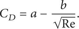
The occurrence of a leak divides the duct system into three parts: exact location, upstream, and downstream, as illustrated in Figure 2. The profiles of pressure and flow rate, over the pipeline, show the leak location. Edrisi and Kam [3] studying gas monophase flow reported that the fluid loss in the leak location can be given by (1), where P_up and T_up represent the pressure and temperature inside the duct and in the leak location, respectively, q_SC and γ_g are the gas flow rate and gas specific gravity at standard conditions, respectively, A is the opening size of the leak, and k is a constant that depends on the material and geometry. The leakage coefficient C_D is given by (2), where a and b are parameters determined by experimental conditions and Re is the Reynolds number. The authors fixed values of flow rate at input and pressure at the output of the duct and compared two permanent states, with and without leakage. The disturbances in the input pressure and in the output flow rate indicate the presence of leakage.

Edrisi and Kam [3] have used experimental results of Scott and Yi (1998) to study the use of the coefficient of leakage (C_D). The experiments consist of a methane gas monophase flow in a horizontal duct with a length of 9.46 ft and an internal diameter of 3.64 in. A range of output pressure values between 610 and 680 psia and a range of gas flow rate injection from 1 to 6 MMscf/Day were assumed as boundary conditions. The leakage is located in the middle of the duct and has its diameter varied in three values equal to 1/8, 1/4, and 3/8 inches. The C_D values range from 0.55 to 4.11. Several data analyses were made and can be seen in detail in Edrisi and Kam [3]. In Figure 1 the behavior of the flow rate and the pressure over the duct is observed. The author concluded that the coefficient of leakage is proportional to Reynolds number, differently from what is shown in (2). Consider the following:

q_{SC} = 879 C_{D} A P_{up} \sqrt{(\frac{k}{γ_{g} T_{up}}) {(\frac{2}{k + 1})}^{(k + 1) / (k - 1)}},

(1)

C_{D} = a - \frac{b}{\sqrt{Re}} .

(2)

Figure 1:

Behavior of pressure and flow rate along the pipeline with a leak.

Figure 2:

Representation of the tube with leak regions.

Zhang et al. [1] say that the method of pipeline leak detection called negative pressure wave (NPW) method is between the three widely used and investigated methods of pipeline leak detection worldwide. Actually leak detection monitoring system (LDMS) based on the NPW method has already been installed on crude oil pipelines more than 20,000 km in China, even though it has been playing a significant role in the pipeline running safety, reducing the false alarm rate. The NPW method has some drawbacks in detecting a slow leak or a small leak, resulting in a lower accuracy in a detection of a leak location. Zhang et al. [1] propose the use of a novel LDMS of long distance oil pipeline based on a dynamic pressure transmitter (DPT) to solve the main problems of signal recognition. For this propose, the authors performed experiments using the oil pipeline of PetroChina, with a pipe length of 94.21 km and a pipe diameter of 457 mm. The pipeline leaks were simulated at a distance of 75.5 km from the inlet station and the dynamic pressure transmitters were installed, respectively, in the inlet and outlet stations. The leak detection monitoring based on DPT is designed utilizing the WPE feature extraction method for pipeline leak judgment. The results show that the pipeline leak detection based on DPT has higher sensitivity and resolution than those of ordinary pressure transmitter. Moreover the leak correct recognition rate of field experiment is 96.7%, and the greatest leak localization error is 101 m.

There are variables in the leak phenomenon that are not so easy to measure in practice. Recently, some authors used the computational fluid dynamic as a tool to help in this process. The cases described below can be cited as examples.

Barbosa et al. [4] simulated the three-phase and nonisothermal flow of oil, water, and gas. The flow domain consists of a vertical duct with a length of 7 meters and a diameter of 12.5 cm. The duct has a leak with a diameter of 8 mm and located at 3.5 m from the input section of the duct. The following parameters were used: velocity of 1 m/s for water and 0.5 m/s for oil and gas and volumetric fraction of 0.8 for oil, 0.15 for water, and 0.05 for gas phase.

The results of numeric simulation showed a disturbance in the temperature field with a leakage. The fluid leak magnitude is proportional to the growth of temperature around them. The pressure drop over the duct was analyzed and it was noticed that the pressure drop is directly proportional to viscosity, initial velocity of oil, and magnitude of leak.

Sousa et al. [5] simulated the flow of a two-phase mixture (water and oil) in a vertical duct with a length of 8 meters and diameter of 15 cm containing a leak with a diameter of 6 mm located 4 m from the input section of the duct. The simulations were run using Ansys CFX. These authors changed the volumetric fraction of oil in the input flow in a range from 0.75 to 1, and they noted that the higher the volume fraction of water in the mixture, the greater the flow passing through the leak orifice.

Tavares [6] studied numerically two types of isothermal flow: two-phase (oil and water) and three-phase (oil, water, and gas), in a horizontal duct with a pipe length of 10 meters and a pipe diameter of 20 cm containing a leak with a diameter of 16 mm located 5 m from the input section of the duct. The effect of the position of the leak orifice (up, lateral, and bottom) and mixture composition (oil fraction from 90% to 80%, water fraction from 5% to 10%, and gas fraction from 0% to 10%) was analyzed.

The results showed an increase of the pressure drop at the first 0.02 s, period without leak. After this time the leak condition was defined, putting a prescribed velocity of 0.06 m/s on the leak orifice surface. Between 0.02 and 0.03 s there was a decrease in a pressure drop and then an increase until a constant value. The cases with a two-phase flow had a smaller variation of the pressure drop than the cases with a three-phase flow.

Araújo et al. [7] used the computational fluid dynamic to simulate a two-phase flow (oil and water) in a duct with leaks, studying how the size of the leak can perturb the hydrodynamic of flow inside the duct and how the volumetric fraction of oil can influence the amount of oil lost. One of the conclusions is the following: by increasing the diameter of the leak orifice, the volume of fluid leaving the orifice is greater.

To evaluate the influence of the leak in a tee junction about the flow dynamics parameter, Araújo et al. [8] simulated the oil flow in a tee junction with one or two leak orifices. The main pipe has a length of 6 m and pipe diameter of 10 cm, while the secondary pipe has the same diameter and has a length of 3 m. There is a leak in the main pipe and another leak in the secondary pipe, both with a diameter of 8 mm. By measurement of the pressure at the inlet section of the main pipe, one of the conclusions of the authors is that the leak in the main pipe causes a bigger disturbance in the pressure field than the leak in the secondary pipe.

In this sense, this paper aims to study the transient dynamic behavior of the oil flow in pipes containing one or two leaks, in terms of velocity and pressure fields, specifically, to analyze the behavior of the flow on the emergence of a leak when there is already another leak in the pipeline.

2. Methodology

2.1. Study Domain

The domain is a horizontal duct with a length of 10 meters and a diameter of 0.2 m. The pipe has two leaks with a diameter of 1.6 cm and located at 5 m and at 7.5 m from the inlet section of the duct, as illustrated in Figure 2.

The mesh utilized in the simulations is shown in Figure 3, beyond the details of the leak and inlet and outlet sections. This mesh has 326768 tetrahedral elements, and it is the result of several refinements to assure the nondependence of the numerical results with the use of this mesh in simulations, as well as a suitable computational cost.

Figure 3:

Representation of the tube mesh and details of sections: (a) leak at x = 5 m, (b) leak at x = 7.5 m, (c) input, (d) output, and (e) one of the leaks.

2.2. Mathematical Modeling

The governing equations to describe the phenomenon of the fluid flow in the pipe and leak are the conservation of mass and momentum represented, considering the Eulerian-Eulerian approach and the following assumptions:

the flow is transient and laminar;

the fluid is Newtonian, incompressible, and with constants thermophysical and chemical properties;

the flow is isothermal;

there is no occurrence of chemical reactions;

the gravitational effect was considered.

The equations that describe the flow were withdrawn from Ansys CFX.

Permanent regime:

mass conservation equation is

\nabla \cdot (ρ U) = 0,

(3)

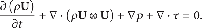
where ρ and U are, respectively, the density and the velocity vector;

momentum conservation equation is

\nabla \cdot (ρ U \otimes U) + \nabla p + \nabla \cdot τ = 0,

(4)

where p is the pressure and τ is the stress tensor.

Transient model:

mass conservation equation is

\frac{\partial ρ}{\partial t} + \nabla \cdot (ρ U) = 0,

(5)

where t is the time;

momentum conservation equation is

\frac{\partial (ρ U)}{\partial t} + \nabla \cdot (ρ U \otimes U) + \nabla p + \nabla \cdot τ = 0 .

(6)

2.3. Initial and Boundary Conditions

2.3.1. Boundary Conditions

The boundary conditions considered on the duct, Figure 2, are given by the following:

in the inlet section: constant oil velocity equal to 0.2, 0.5, or 1.0 m/s according to the case shown in Table 1;

in the outlet section: constant static pressure equal to 101325 Pa;

in the duct wall: no slip conditions, U_x = U_y = U_z = 0 m/s;

in the leak(s): five conditions were used.

When there is no leakage in the two orifices

leak 1 is closed: no flow, U_x = U_y = U_z = 0 m/s;

leak 2 is closed: no flow, U_x = U_y = U_z = 0 m/s.

When there is leakage in the first orifice (leak 1) only

leak 1 is opened: average static pressure equal to 101325 Pa;

leak 2 is closed: no slip, U_x = U_y = U_z = 0 m/s.

When there is leakage in the second orifice (leak 2) only

leak 1 is closed: no flow, U_x = U_y = U_z = 0 m/s;

leak 2 is opened: average static pressure equal to 101325 Pa.

When there is leakage in the first orifice and after 1.6 seconds there is leakage too in the second orifice.

For 0 ≤ t ≤ 1.6 s

leak 1 is opened: average static pressure equal to 101325 Pa;

leak 2 is closed: no flow, U_x = U_y = U_z = 0 m/s.

For t > 1.6 s

leak 1 is opened: average static pressure equal to 101325 Pa;

leak 2 is opened: average static pressure equal to 101325 Pa.

When there are leaks in the two orifices

leak 1 is opened: average static pressure equal to 101325 Pa;

leak 2 is opened: average static pressure equal to 101325 Pa.

Table 1:

Data used in the simulations.

Case	Oilvelocity [m/s]	Leak at 5 m from inlet section (leak 1)		Leak at 7.5 m from inlet section (leak 2)
Case	Oilvelocity [m/s]	Leak 1	t [s]	Leak 2	t [s]

01	0.2	U_x = U_y = U_z = 0	0	U_x = U_y = U_z = 0	0
02	0.2	U_x = U_y = U_z = 0	0	U_x = U_y = U_z = 0	0
03	0.2	U_x = U_y = U_z = 0	0	U_x = U_y = U_z = 0	0
04	0.2	U_x = U_y = U_z = 0	0	U_x = U_y = U_z = 0	0

05	0.5	101325 Pa	0	U_x = U_y = U_z = 0	0
06	0.5	U_x = U_y = U_z = 0	0	101325 Pa	0
07	0.5	101325 Pa	0	101325 Pa	1.6
08	0.5	101325 Pa	0	101325 Pa	0
09	1.0	101325 Pa	0	U_x = U_y = U_z = 0	0
10	1.0	U_x = U_y = U_z = 0	0	101325 Pa	0
11	1.0	101325 Pa	0	101325 Pa	1.6
12	1.0	101325 Pa	0	101325 Pa	0

2.3.2. Initial Conditions

For all cases the numerical results of the simulation of oil laminar flow in steady state without leakage like initial condition were adopted, having an inlet oil velocity of 0.5 m/s (Cases 05 to 08) and 1.0 m/s (Cases 09 to 12), a condition of no slip in the wall and in the leak, and static pressure of 101325 Pa in the outlet section of the pipe.

Optimizing the simulation time to minimize the occupation of memory in the hardware and to obtain accuracy in the results, the time step was changed throughout the simulation. From 0 to 0.01 s of flow the time step was 0.001 s, from 0.001 s to 0.1 s the value of the time step was 0.01 s, from 0.1 s to 1 s the time step was 0.1 s, and after 1 s of the flow the time step was 0.2 s. The exception occurred for Cases 07 and 11, where in the instant 1.6 s there is a new leak orifice, and the time step was reduced to 0.001 s; from 1.61 s to 1.7 s the step increased to 0.01 s, from 1.7 to 2.6 s the step was 0.1 s, and from 2.6 s to 3.2 s the time step was 0.2 s.

Data for the studied cases are shown in Table 1.

2.4. Fluid Data

The properties of the oil used in the present work are shown in Table 2.

Table 2:

Oil properties.

Properties	Oil	Source

Density (kg/m³)	868.7	Cunha [9]
Molar mass (kg/kmol)	105.47	Cunha [9]
Viscosity (Pa·s)	0.17	Cunha [9]

2.5. Mesh Refinement Study

The mesh dependence was analyzed by the refinement of the mesh in four different levels (Table 3). The convergence criterion adopted was the root mean square with a residual target of 10⁻⁸.

Table 3:

Meshes used in the refining study.

Case	Mesh	Number of hexahedral elements	Number of nodes

01	1	144694	138904
02	2	206894	199926
03	3	281810	273282
04	4	309720	300482

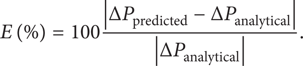
The parameter used to choose the mesh was the pressure drop. The analytical value of the pressure difference in a section of the duct with the length of 1 m was calculated from Darcy-Weisbach equation (7), where f is the friction factor. The numerical value of the pressure difference in a section of the duct with the length of 1 m was calculated from the difference between the calculated average pressure in the cross-section yz in x = 3 m and in the cross-section yz in x = 4 m (fully developed region). The relative error between analytical and numerical values is calculated from (8), where ΔP_predicted is the numerical value and ΔP_analytical is the analytical value. Consider

\frac{Δ P}{L} = \frac{f}{D} \frac{ρ U^{2}}{2},

(7)

E (%) = 100 \frac{|Δ P_{predicted} - Δ P_{analytical}|}{|Δ P_{analytical}|} .

(8)

3. Results and Discussion

3.1. Dependence of the Mesh and Validation

The values of pressure differences in the pipe section are shown in Table 4. The results indicate that there is virtually no variation between Cases 03 and 04.

Table 4:

Pressure difference as a function of the density of control volumes in the mesh.

Case	ΔP analytical[Pa]	ΔP predicted[Pa]	Percentual error

01	17 Pa	16 Pa	6.25%
02	17 Pa		6.25%
03	16 Pa		0.00%
04	16 Pa		0.00%

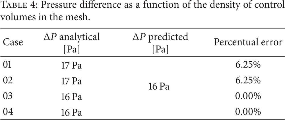
Based on these results, the mesh for Case 03 was chosen for the next simulations, because this case gives good results and a lower computational cost (lower computational time) comparing with Case 4. Further, results presented in Table 4 can be used for validation of the mesh and mathematical modeling presented in this work.

3.2. Leaks in Pipeline

3.2.1. Velocity Analysis

Figure 4 shows the behavior of oil velocity field on the longitudinal plane xy for Cases 08 and 12 (Table 1), after the flow regime reaches a permanent regime. In the details of leak region, there is a disorder in the velocity profile caused by leakage. Note that the region of leak 1 (at 5.0 m from inlet section) presents a bigger velocity than the region of leak 2 (at 7.5 m from inlet section). This behavior explains the reason of escape of a bigger volume of fluid through leak 1 than through leak 2.

Figure 4:

Velocity field. (a) Case 08 and (b) Case 12.

Figure 5 shows the velocities in the leak orifices changing with time. It is clear to notice how the presence of a new leak perturbs the velocity field around the previous leak. In Figures 6 and 7 the streamlines and the velocity vector fields are shown at 3.2 s.

Figure 5:

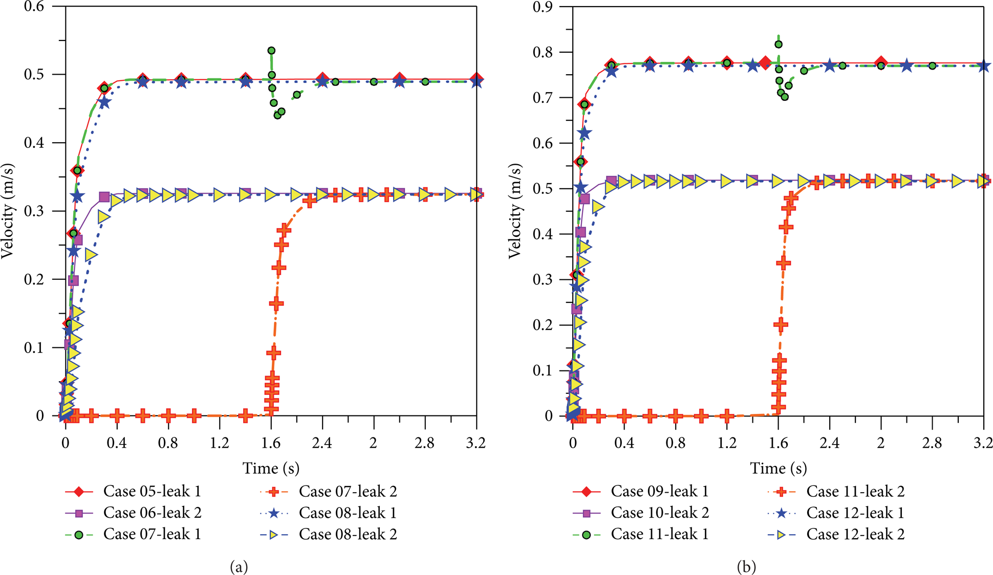
Velocity in the leak orifice. (a) Cases 05, 06, 07, and 08 and (b) Cases 09, 10, 11, and 12.

Figure 6:

Streamlines and vectors representing the velocity fields. (a) Case 05, (b) Case 06, and (c) Case 08.

Figure 7:

Streamlines and vectors representing the velocity fields. (a) Case 09, (b) Case 10, and (c) Case 12.

3.2.2. Pressure Analysis

Figure 8 shows the field of pressure on the xy longitudinal plane, for Cases 08 and 12 (Table 2), after the flow regime to acquire a permanent regime (3.2 s). In the details of leak region there is a variation in the pressure caused by leakage. Leak 1 shows a higher pressure in the neighborship than leak 2. It occurs due to leak 1 being closer to the inlet section, region in the pipe with the higher pressure, than leak 2.

Figure 8:

Pressure field. (a) Case 08 and (b) Case 12.

Figure 9 illustrates the pressure fields of Cases 08 and 12, respectively, in one axial plane and in two transverse planes passing the center of leak orifice. A discontinuity of the pressure distribution illustrating a pressure gradient toward the output of the fluid in the leak orifices is noticed.

Figure 9:

Pressure field on the axial plane and cross planes (x = 5 m and x = 7.5 m) in t = 3.2 s. (a) Case 08 and (b) Case 12.

Figures 10, 11, and 12 show the average pressures, measured at input section, changing with time. There is, in the first moments of flow, presence of a sharp decline of pressure caused by leak, followed by a sudden increase in pressure.

Figure 10:

Pressure evolution at the inlet section of the pipe as a function of the time (Cases 05, 06, 09, and 10).

Figure 11:

Pressure evolution at the inlet section of the pipe as a function of time (Cases 07, 08, 11, and 12).

Figure 12:

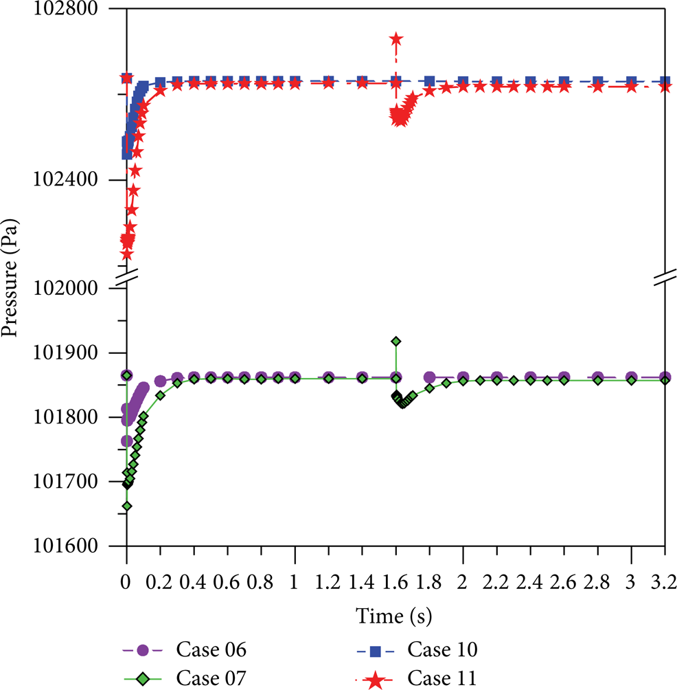
Pressure evolution at the inlet section of the pipe as a function of time (Cases 06, 07, 10, and 11).

It is visible in Figure 10 that the place of leak orifice provokes pressure variations caused by leak. The pressure drop due to the leak at 5 m from input (Cases 05 and 09) is bigger than drop due to the leak at 7.5 m from input (Cases 06 and 10).

The results shown in Figure 11 are a comparison between the situations where the two leaks are activated at the beginning of the simulation (Cases 08 and 12) and the situation where leak 1 is initialized at 0 s (the leak located at 5 m from input) and leak 2 after 1.6 s (the leak located at 7.5 m from input) (Cases 07 and 11). The time 1.6 s was chosen due to the fact that this time is enough to stabilize the pressure. It is observed that, regardless of the time of onset of leakage, if they have the same diameter and are located in the same regions, the final pressure measured in a particular section, after stabilizing the pressure, will be dependent on the inlet conditions (pressure or velocity specified).

It is noted in Figure 12 how a presence of one leak can influence the detection of another. In Cases 06 and 10 leak 2 was activated when there is no leakage before, causing disturbances in the pressure at the inlet section of the pipe. However, if leak 1 was opened previously (at 5 m), the activation of leak 2 at 1.6 s (Cases 07 and 11) causes a smaller disturbance in pressure comparing to the situation where leak 2 exists alone, and it occurs because the pressure measured at the inlet section is small around the time of 1.5 s for Cases 06 and 10.

4. Conclusions

Based on the results the following conclusions are described:

the mesh used presented results that do not depend on their sophistication, being classified as able to be used in the simulations;

the leakage causes a disturbance on the fields of velocity and pressure along the flow;

the leak closest to the duct entrance has provoked the greatest pressure drop measured at the inlet section of the pipe;

a pipeline containing two or more leaks has the same pressure measured at the input section regardless of the time of opening of the leaks and inlet fluid velocity;

the pressure drop due to the presence of a leak may vary according to other preexisting leaks in the pipe, which makes their detection difficult.

Conflict of Interests

The authors declare that there is no conflict of interests regarding the publication of this paper.

Footnotes

Acknowledgments

The authors would like to express their thanks to CAPES, CNPq, FINEP, PETROBRAS, ANP/UFCG/PRH-25, and RPCMOD for supporting this work and are also grateful to the authors of the references cited in this paper that helped in the improvement of quality.

References

Zhang

Chen

, and Jin

, “Leak detection monitoring system of long distance oil pipeline based on dynamic pressure transmitter,” Measurement, vol. 49, no. 1, pp. 382–389, 2014.

Agbakwuru

, “Oil/gas pipeline leak inspection and repair in underwater poor visibility condititons: challenges and perspectives,” Journal of Environmental Protection, vol. 3, no. 5, pp. 394–399, 2012.

Edrisi

and Kam

S. I.

, “Mechanistic leak-detection modeling for single gas-phase pipelines: lessons learned from fit to field-scale experimental data,” Advances in Petroleum Exploration and Development, vol. 5, no. 1, pp. 22–36, 2013.

Barbosa

L. M. C.

de Lima

A. G. B.

, and de Farias Neto

S. R.

, “Non-isothermal transient three-phase flow (heavy oil, water and gas) in vertical pipeline: the effect of leakage,” International Journal of Modeling and Simulation for Petroleum Industry, vol. 6, no. 12, pp. 23–31, 2012.

Sousa

J. V. N.

de Lima

A. G. B.

, and de Farias Neto

S. R.

, “Numerical analysis of heavy oil-water flow and leak detection in vertical pipeline,” Advances in Chemical Engineering and Science, vol. 3, no. 1, pp. 9–15, 2013.

Tavares

D. P. S. A.

, Non-isothermal three-phase flow in horizontal ducts with leakage: modeling and simulation [M.S. thesis], Federal University of Campina Grande, Campina Grande, Brazil, 2012, (Portuguese).

Araújo

Neto

, and Lima

, “Theoretical evaluation of two-phase flow in a horizontal duct with leaks,” Advances in Chemical Engineering and Science, vol. 3, no. 4, pp. 6–14, 2013.

Araújo

de Luna

F. D. T.

Barbosa

E. S.

Neto

, and Lima

, “Numerical study of oil flow in tee junction with leaks,” Advances in Petroleum Exploration and Development, vol. 6, no. 2, pp. 1–11, 2013.

Cunha

A. L.

, Non-isothermal enhanced recovery of heavy oil in petroleum reservoirs via numerical simulation [Dissertation] (Master in Chemical Engineering), Federal University of Campina Grande, Campina Grande, Brazil, 2010, (Portuguese).

Hydrodynamic Study of Oil Leakage in Pipeline via CFD

Abstract

1. Introduction

2. Methodology

2.1. Study Domain

2.2. Mathematical Modeling

2.3. Initial and Boundary Conditions

2.3.1. Boundary Conditions

2.3.2. Initial Conditions

2.4. Fluid Data

2.5. Mesh Refinement Study

3. Results and Discussion

3.1. Dependence of the Mesh and Validation

3.2. Leaks in Pipeline

3.2.1. Velocity Analysis

3.2.2. Pressure Analysis

4. Conclusions

Conflict of Interests

Footnotes

Acknowledgments

References