Sensitivity Analysis of the Transmission Chain of a Horizontal Machining Tool Axis to Design and Control Parameters

Abstract

This paper reports how a numerical controlled machine axis was studied through a lumped parameter model. Firstly, a linear model was derived in order to apply a modal analysis, which estimated the first mechanical frequency of the system as well as its damping coefficients. Subsequently, a nonlinear system was developed by adding friction through experimentation. Results were validated through the comparison with a commercial servoaxis equipped with a Siemens controller. The model was then used to evaluate the effect of the stiffness of the structural parts of the axis on its first natural frequency. It was further used to analyse precision, energy consumption, and axis promptness. Finally a cost function was generated in order to find an optimal value for the main proportional gain of the position loop.

1. Introduction

In the past, numerical controlled machines were intended to produce small batches. Moreover, nowadays even middle to large amounts of units are being produced using numerical controlled machines. Thus there is an increasing presence of these machines in industry spread across all economic sectors and levels of production. The market demands high precision and short production times. Machines must be as stiff as possible and must be able to work at high capacity but must have low energy consumption.

All the above desirable features may be studied through mathematical models. These can estimate the behaviour of the machine before its construction. Furthermore, once a machine is created, a physical alteration of the system is not required if models are used to study new configurations. Several authors have used mathematical models to analyse or design controlled numerical machines. In [1] a lumped parameter model was created to quantify the sensitivity of each vibration mode to a variation in the stiffness of the kinematic chain of a rotary table transmission. The former model was also mixed with an object-oriented model to consider the nonlinearities of the system. Sato [2] also proposed and validated a model of a rotary table with a worm gear. Jeong and You [3] studied the position synchronous control of a multiaxis servo system without hard couplings. To do so a model of the motor drive was formulated using circuit equations and Newton's laws. Some models have been defined using hybrid approaches [4–6] in which lumped and distributed modelling are combined. A model using robotics formalism was adopted in [7] as a new way of modelling machine tools.

In this analysis an axis was discretized into lumped bodies linked to each other by springs and dampers. The stiffness of each spring was calculated using mathematical correlations with both dimensional characteristics and material properties. The damping coefficients were estimated based on an assumption of structural damping. Friction was then identified using the procedure described in [8]. Subsequently, the dynamic equilibrium equation of each body was written and a system of equations was assembled adding the equations that came from the control action. These equations were then solved for different reference commands. Three aspects of the system were used to determine the reliability of the results: bode diagrams in frequency domain and, in time domain, position response and torque.

Finally, once the axis model was validated, it was used to carry out a sensitivity analysis of the servoaxis performance to peculiar design and control issues. In particular, in this work the effects of the stiffness of the metal support of the axis on its first modal frequency are investigated. Furthermore, a methodological criterion to optimize the main proportional gain of the control loop in terms of precision, velocity, and energy consumption is presented.

2. General Description of the Machine

The axis studied is part of a commercial numerical controlled machine with a Cartesian structure. The main objective of the axis is to position the tool used to contour the raw material longitudinally. Position errors lead to larger tolerances that negatively affect the final result.

The axis is disposed in a rotary screw arrangement (Figure 1). A ball screw is mounted on a roller pack fixed to a metal support. The system is operated by a brushless motor coupled to the ball screw through an elastic joint to avoid issues due to misalignments. The ball nut is fixed to the slide; in this manner, the turning of the screw generates a linear movement of the slide. The slide is equipped with recirculating rolling guides to constrain all degrees of freedom but the desired travel direction.

Figure 1:

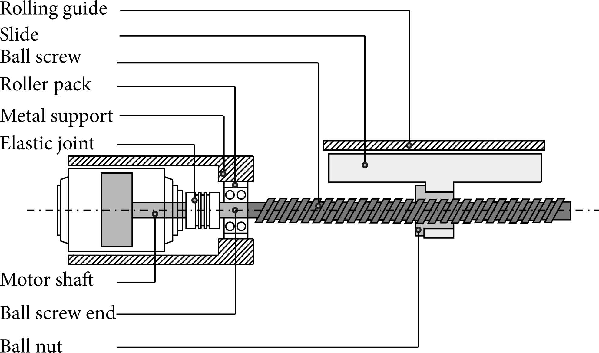
Rotary screw arrangement.

3. Mathematical Modelling

A lumped parameter model was created. By identifying all the rigid bodies with inertia, it was possible to establish the degrees of freedom of the system, that is, the rotation and axial displacement of each body. All the bodies were connected to each other by means of elastic and damping elements. Starting from a realistic representation of the axis (Figure 1), the model in Figure 2 was assembled. In the former figure, two subsystems are identified: a rotary subsystem, which comprises the motor shaft, ball screw end, and ball screw, and an axial subsystem conformed by the ball screw, ball nut, and the slide. The shaft of the motor is connected to the ball screw end through a spring plus a damper. These elements represent the stiffness and damping coefficient of the shaft plus the elastic joint in series. After it, the ball screw end and the ball screw are interfaced by an element that includes their stiffness and damping coefficient.

Figure 2:

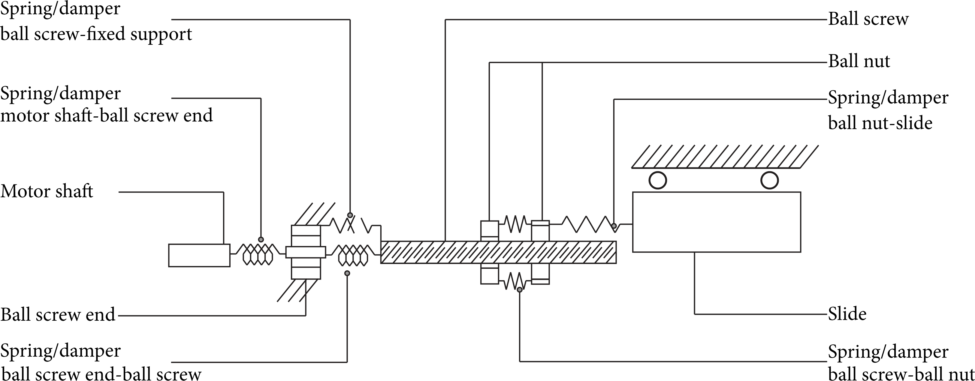
Schematic view of the axis.

The lead of the ball screw is given by its geometry. Since the subsystem conformed by the inner race, the balls, and the outer race of the ball screw-ball nut coupling is not infinitely rigid, the actual displacement of the ball nut will not be equal to that computed based on the geometry of the screw. For that reason the element “spring/damper ball screw-ball nut” was introduced in Figure 2. The left part of the ball nut has no mass; it takes into account the geometric lead. All the mass of the ball nut was assigned to the right part. The displacement of this part will be the effective travel of the nut given the compliance of the coupling. From the ball screw, through its flange, the forces are transferred to the slide where the spindles are. The element “Spring/damper ball nut-slide” represents the stiffness of the flange of the nut.

Finally, the compliance of the support of the axis was also considered: it is represented by “spring/damper ball screw-fixed support” in Figure 2. The resulting series of three springs and dampers gives the value of this element: the axial stiffness/damping of the ball screw plus the axial stiffness/damping of the bearing plus the axial stiffness/damping of the metal support of the axis.

Once the scheme of the model was created, two sets of differential equations, the axial and rotational equilibrium equations of each rigid body with inertia, were formulated to describe the dynamics of the axis. Moreover, the actuator of the system was modelled as a DC motor driven by a position and velocity control loop hardware.

The main hypothesis formulated in order to reduce the complexity of the model is detailed below:

• the friction force introduced by the recirculating rolling guides on the slide was neglected;

• the friction torque introduced by the bearing pack on the ball screw end was also neglected;

• all the friction effects were concentrated on the ball screw-ball nut coupling because of the preload of the ball nut.

3.1. Control Scheme

Figure 3 summarizes the position and control loop architecture. In the stage of position control the automatic controller and the sensor have a proportional (P) behaviour. The deviation between position command and feedback is amplified by means of the proportional gain of the position loop k _v . The position command is also transformed into velocity command compensation (feed-forward): the position reference is differentiated and multiplied by the feed-forward gain k_FF. The speed/velocity loop has a proportional-plus-integrative (PI) controller: the error between the velocity reference and its actual value is divided into two branches. One of them is multiplied by the gain k _p and the other multiplied by k _i and then integrated. Finally, the sum of the branches becomes the voltage reference to the motor.

Figure 3:

Position and velocity control loop.

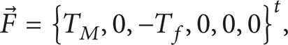
To model the actuator the following equations were used:

$\begin{array}{c}{V}_a=R{i}_a+L\frac{d}{dt}{i}_a+k_e{\dot{\theta }}_{\mathrm{1}},\\ T_M=k_T{i}_a,\end{array}$

(1)

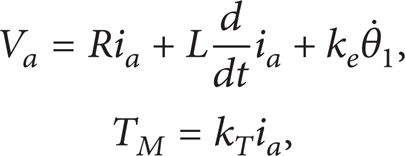
where i _a is the torque-generating current, V _a is the armature voltage, T _M is the motor torque, R is the electric resistance, L is the inductance, k _e and k _T are the electrical constant and torque constant, respectively, and θ₁ is the angular position of the motor shaft.

3.2. Rotary Subsystem

The lumped model of the transmission from the motor shaft to the ball screw is illustrated in Figure 4. The motor torque spins the rotor which is connected through an elastic/damping joint to the ball screw end. The ball screw end is treated as a separate element from the ball screw itself due to geometrical differences, and an elastic/damping linkage between them is modelled.

Figure 4:

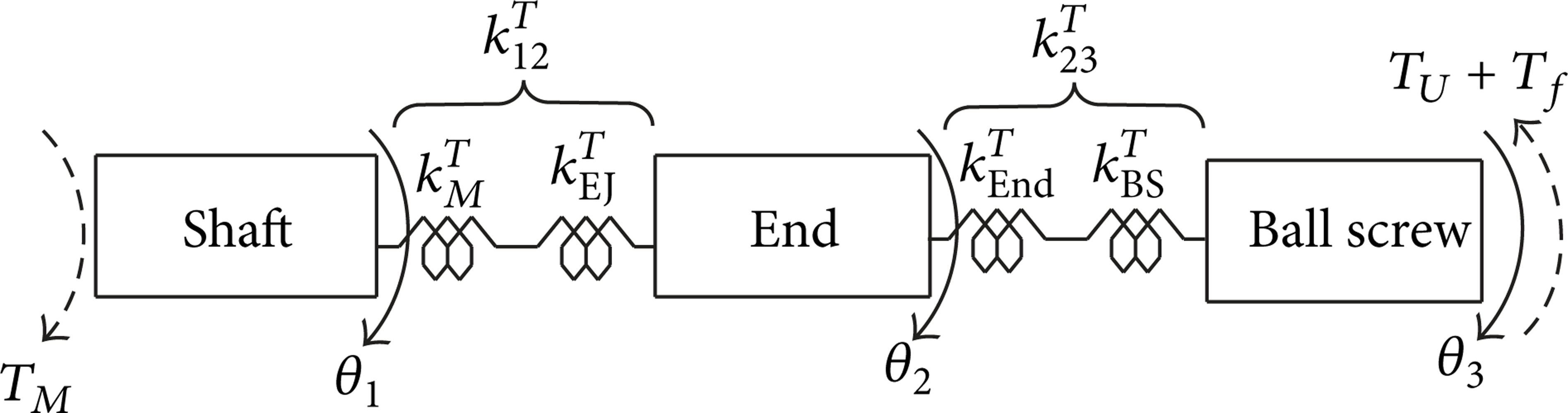
Rotary elements.

3.2.1. Motor Shaft

The dynamic equilibrium equation of the motor shaft

$T_M=J_M{\ddot{\theta }}_{\mathrm{1}}+{\beta }_{\mathrm{12}}^T\left({\dot{\theta }}_{\mathrm{1}}-{\dot{\theta }}_{\mathrm{2}}\right)+k_{\mathrm{12}}^T\left({\theta }_{\mathrm{1}}-{\theta }_{\mathrm{2}}\right)$

(2)

with

$k_{\mathrm{12}}^T={\left(\frac{\mathrm{1}}{k_M^T}+\frac{\mathrm{1}}{k_{\text{EJ}}^T}\right)}^{-\mathrm{1}}$

(3)

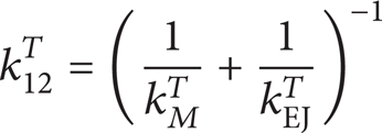
is derived from Figure 4, where θ₁ and θ₂ are the angular position of the shaft and ball screw end, respectively, J _M is the moment of inertia of the rotor plus half of the elastic joint, k _M ^T and k_EJ ^T are the torsional stiffness of the motor shaft and the elastic joint, and β₁₂ ^T is the resulting torsional damping coefficient between θ₁ and θ₂.

3.2.2. Ball Screw End

Through the elastic/damping joint, the torque is transmitted from the shaft of the motor to the ball screw end. The dynamic equilibrium equation of the ball screw end is

$\begin{array}{c}{\beta }_{\mathrm{12}}^T\left({\dot{\theta }}_{\mathrm{1}}-{\dot{\theta }}_{\mathrm{2}}\right)+k_{\mathrm{12}}^T\left({\theta }_{\mathrm{1}}-{\theta }_{\mathrm{2}}\right)\hfill \\ \hspace{1em}=J_{\text{END}}{\ddot{\theta }}_{\mathrm{2}}+{\beta }_{\mathrm{23}}^T\left({\dot{\theta }}_{\mathrm{2}}-{\dot{\theta }}_{\mathrm{3}}\right)+k_{\mathrm{23}}^T\left({\theta }_{\mathrm{2}}-{\theta }_{\mathrm{3}}\right)\end{array}$

(4)

with

$k_{\mathrm{23}}^T={\left(\frac{\mathrm{1}}{k_{\text{END}}^T}+\frac{\mathrm{1}}{k_{\text{BS}}^T}\right)}^{-\mathrm{1}}.$

(5)

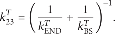
In (4) θ₃ is the angular position of the ball screw, J_END is the moment of inertia of the ball screw end plus half of the elastic joint, k_END ^T and k_BS ^T are the torsional stiffness of the ball screw end and ball screw, respectively, and β₂₃ ^T is the torsional damping coefficient between θ₂ and θ₃.

3.2.3. Ball Screw

The ball screw delivers a useful torque T _U that, through the pair screw/nut, becomes the axial force needed to move the slide. The dynamic equilibrium equation of the ball screw is

${\beta }_{\mathrm{23}}^T\left({\dot{\theta }}_{\mathrm{2}}-{\dot{\theta }}_{\mathrm{3}}\right)+k_{\mathrm{23}}^T\left({\theta }_{\mathrm{2}}-{\theta }_{\mathrm{3}}\right)=J_{\text{BS}}{\ddot{\theta }}_{\mathrm{3}}+T_U+T_f.$

(6)

The constant J_BS is the moment of inertia of this element. As mentioned in Section 2, the friction torque T _f due to preload was considered to be acting on this body.

3.3. Axial Subsystem

The elements considered that undergo axial displacement are the slide, the ball nut, and the ball screw due to the compliance of the metal support of the axis (Figure 5). The former is an undesired effect that decreases the precision of the axis.

Figure 5:

Travelling elements.

3.3.1. Ball Screw

The support of the axis yields under load. The ball screw travels with it due to the axial force F _U between ball screw and nut. This force and the useful torque are related in the following fashion:

$F_U=\frac{\mathrm{2}\pi }{p}{T}_U,$

(7)

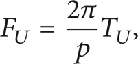
where p is the lead of the ball screw.

The expression of the dynamic equation of the axial displacement of the ball screw is

${-F_U=m}_{\text{BS}}{\ddot{x}}_{\mathrm{0}}+{\beta }_{\mathrm{0}}^A{\dot{x}}_{\mathrm{0}}+k_{\mathrm{0}}^A{x}_{\mathrm{0}}$

(8)

with

${k_{\mathrm{0}}^A=\left(\frac{\mathrm{1}}{k_S^A}+\frac{\mathrm{1}}{k_B^A}+\frac{\mathrm{1}}{k_{\text{BS}}^A}\right)}^{-\mathrm{1}}.$

(9)

In (8) and (9) x₀ is the axial displacement of the ball screw, m_BS is the mass of the ball screw, k _S ^A , k _B ^A , k_BS ^A are, respectively, the axial stiffness of the support, bearing pack, and ball screw, and β₀ ^A is the resulting axial damping coefficient between x₀ and the fixed ground.

3.3.2. Ball Nut

Because of the yielding of the screw support under load, the ball nut will travel a distance slightly different from its lead for a single revolution. The theoretical axial displacement of the nut due to the transmission ratio of the pair screw/nut taking into account the displacement x₀ is

$x_{\mathrm{1}}=x_{\mathrm{0}}+{\theta }_{\mathrm{3}}h$

(10)

with

$h\mathrm{\hspace{0.17em}\hspace{0.17em}}=\frac{p}{\mathrm{2}\pi }.$

(11)

In order to take into account the axial compliance of the system formed by the inner race of the screw, the balls, and the outer race of the nut, a spring/damper with stiffness k₁₂ ^A and resulting damping coefficient β₁₂ ^A was introduced.

Denoting with x₂ the actual degree of freedom of the nut, the force F _U between ball screw and nut loads the spring/damper element of the nut model; thus

$F_U={\beta }_{\mathrm{12}}^A\left({\dot{x}}_{\mathrm{1}}-{\dot{x}}_{\mathrm{2}}\right)+k_{\mathrm{12}}^A\left(x_{\mathrm{1}}-x_{\mathrm{2}}\right).$

(12)

Finally, the dynamic axial equilibrium equation of the body representing the mass of the ball nut is

$\begin{array}{c}{\beta }_{\mathrm{12}}^A\left({\dot{x}}_{\mathrm{1}}-{\dot{x}}_{\mathrm{2}}\right)+k_{\mathrm{12}}^A\left(x_{\mathrm{1}}-x_{\mathrm{2}}\right)\\ \hspace{1em}\hspace{1em}\hspace{1em}=m_{\text{BN}}{\ddot{x}}_{\mathrm{2}}+{\beta }_{\mathrm{23}}^A\left({\dot{x}}_{\mathrm{2}}-{\dot{x}}_{\mathrm{3}}\right)+k_{\mathrm{23}}^A\left(x_{\mathrm{2}}-x_{\mathrm{3}}\right)\end{array}$

(13)

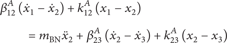
in which x₃ is the displacement of the slide, m_BN is the mass of the ball nut, k₂₃ ^A is the axial stiffness of the flange that connects the ball nut to the slide, and β₂₃ ^A is the axial damping coefficient between x₂ and x₃.

3.3.3. Slide

The dynamic axial equilibrium equation of the slide without any axial load is given by

${\beta }_{\mathrm{23}}^A\left({\dot{x}}_{\mathrm{2}}-{\dot{x}}_{\mathrm{3}}\right)+k_{\mathrm{12}}^A\left(x_{\mathrm{2}}-x_{\mathrm{3}}\right)=m_S{\ddot{x}}_{\mathrm{3}},$

(14)

where the constant m _S is the mass of the slide.

4. Modal Analysis

Putting together equations from (2) to (14) the expression

$M\frac{d^{\mathrm{2}}}{d{t}^{\mathrm{2}}}\overrightarrow{X}+B\frac{d}{dt}\overrightarrow{X}+K\overrightarrow{X}=\overrightarrow{F}$

(15)

may be written. Equation (15) shows the system of equilibrium equations on its matrix form. The vector $\overrightarrow{X}$ comprises the degrees of freedom of the model

$\overrightarrow{X}={\left\{{\theta }_{\mathrm{1}},{\theta }_{\mathrm{2}},{\theta }_{\mathrm{3}},x_{\mathrm{0}},x_{\mathrm{2}},x_{\mathrm{3}}\right\}}^t$

(16)

while the vector $\overrightarrow{F}$ is the force vector

$\overrightarrow{F}={\left\{T_M,\mathrm{0},-T_f,\mathrm{0,0},\mathrm{0}\right\}}^t,$

(17)

and M, B, and K are mass, damping, and stiffness matrices, respectively. It is straightforward to find the matrices M, B, and K; these are given by

$\begin{array}{c}M=\mathrm{diag}\left(J_M,J_{\text{EJ}},J_{\text{BS}},m_{\text{BS}},m_{\text{BN}},m_S\right)\\ K=\left(\begin{array}{cccccc}{k}_{\mathrm{12}}^T& -k_{\mathrm{12}}^T& \mathrm{0}& \mathrm{0}& \mathrm{0}& \mathrm{0}\\ -k_{\mathrm{12}}^T& k_{\mathrm{12}}^T+k_{\mathrm{23}}^T& -k_{\mathrm{23}}^T& \mathrm{0}& \mathrm{0}& \mathrm{0}\\ \mathrm{0}& -k_{\mathrm{23}}^T& k_{\mathrm{23}}^T+h^{\mathrm{2}}{k}_{\mathrm{12}}^A& h{k}_{\mathrm{12}}^A& {-hk}_{\mathrm{12}}^A& \mathrm{0}\\ \mathrm{0}& \mathrm{0}& h{k}_{\mathrm{12}}^A& k_{\mathrm{0}}^A+k_{\mathrm{12}}^A& -k_{\mathrm{12}}^A& \mathrm{0}\\ \mathrm{0}& \mathrm{0}& {-hk}_{\mathrm{12}}^A& -k_{\mathrm{12}}^A& k_{\mathrm{12}}^A+k_{\mathrm{23}}^A& -k_{\mathrm{23}}^A\\ \mathrm{0}& \mathrm{0}& \mathrm{0}& \mathrm{0}& -k_{\mathrm{23}}^A& k_{\mathrm{23}}^A\end{array}\right)\\ B=\left(\begin{array}{cccccc}{\beta }_{\mathrm{12}}^T& -{\beta }_{\mathrm{12}}^T& \mathrm{0}& \mathrm{0}& \mathrm{0}& \mathrm{0}\\ -{\beta }_{\mathrm{12}}^T& {\beta }_{\mathrm{12}}^T+{\beta }_{\mathrm{23}}^T& -{\beta }_{\mathrm{23}}^T& \mathrm{0}& \mathrm{0}& \mathrm{0}\\ \mathrm{0}& -{\beta }_{\mathrm{23}}^T& {\beta }_{\mathrm{23}}^T+h^{\mathrm{2}}{\beta }_{\mathrm{12}}^A& h{\beta }_{\mathrm{12}}^A& {-h\beta }_{\mathrm{12}}^A& \mathrm{0}\\ \mathrm{0}& \mathrm{0}& h{\beta }_{\mathrm{12}}^A& {\beta }_{\mathrm{0}}^A+{\beta }_{\mathrm{12}}^A& -{\beta }_{\mathrm{12}}^A& \mathrm{0}\\ \mathrm{0}& \mathrm{0}& {-h\beta }_{\mathrm{12}}^A& -{\beta }_{\mathrm{12}}^A& {\beta }_{\mathrm{12}}^A+{\beta }_{\mathrm{23}}^A& -{\beta }_{\mathrm{23}}^A\\ \mathrm{0}& \mathrm{0}& \mathrm{0}& \mathrm{0}& -{\beta }_{\mathrm{23}}^A& {\beta }_{\mathrm{23}}^A\end{array}\right).\end{array}$

(18)

To estimate the numeric values of matrix B, some assumptions must be done. In this particular work the damping was supposed to be only structural; that is,

$B=bK,$

(19)

where b is a constant of proportionality between damping and stiffness matrices.

Assuming an undamped system and free oscillations, (15) becomes

$M\frac{d^{\mathrm{2}}}{d{t}^{\mathrm{2}}}\overrightarrow{X}+K\overrightarrow{X}=\overrightarrow{\mathrm{0}}.$

(20)

The undamped frequencies of the system may be calculated by solving the eigenvalue-eigenvector problem in (20) (see [9]). Then the system may be transformed into its modal form and by choosing a value for the modal damping ratio ζ given a modal frequency ω of interest, the constant b may be estimated

$b=\frac{\mathrm{2}\zeta }{\omega }.$

(21)

5. Model Identification

The constants of the model have been shown so far in a nonexplicit way. Several masses, moments of inertia, stiffness, damping coefficients, and the transmission ratio have been introduced throughout this work. This section describes the methods used to estimate all the constants that appear in the model of the system.

Almost all the masses and moments of inertia were found in the parts catalogues. In some cases, such as for the ball screw, they were calculated using the material density and geometric features.

Only the stiffness of the motor shaft was found in the actuator catalogue. For all the other elements, the stiffness was computed, considering the geometry and material properties by means of CAD models of the parts.

The metal support of the axis is a complex part. The stiffness of this element was estimated using the finite element method. By applying different forces and calculating the displacement of a reference point, it was possible to identify an equivalent concentrated stiffness.

Using the masses, the moments of inertia and the stiffness matrices M and K were calculated. The first nonnull frequency of the system ω found was 152 Hz. The former frequency was calculated, considering the ball nut at the middle of the stroke of the axis. It is important to mention it because the stiffness of the ball screw is a function of the ball nut position.

By assuming only structural damping and a 3% modal damping ratio ζ for the first modal frequency ω, the damping matrix was calculated using (19) and (21).

The friction torque T _f was added to the system as an experimental curve function of the speed of the ball screw ${\dot{\theta }}_3$ . By measuring the torque-generating current for different constants speeds, Figure 6 was generated.

Figure 6:

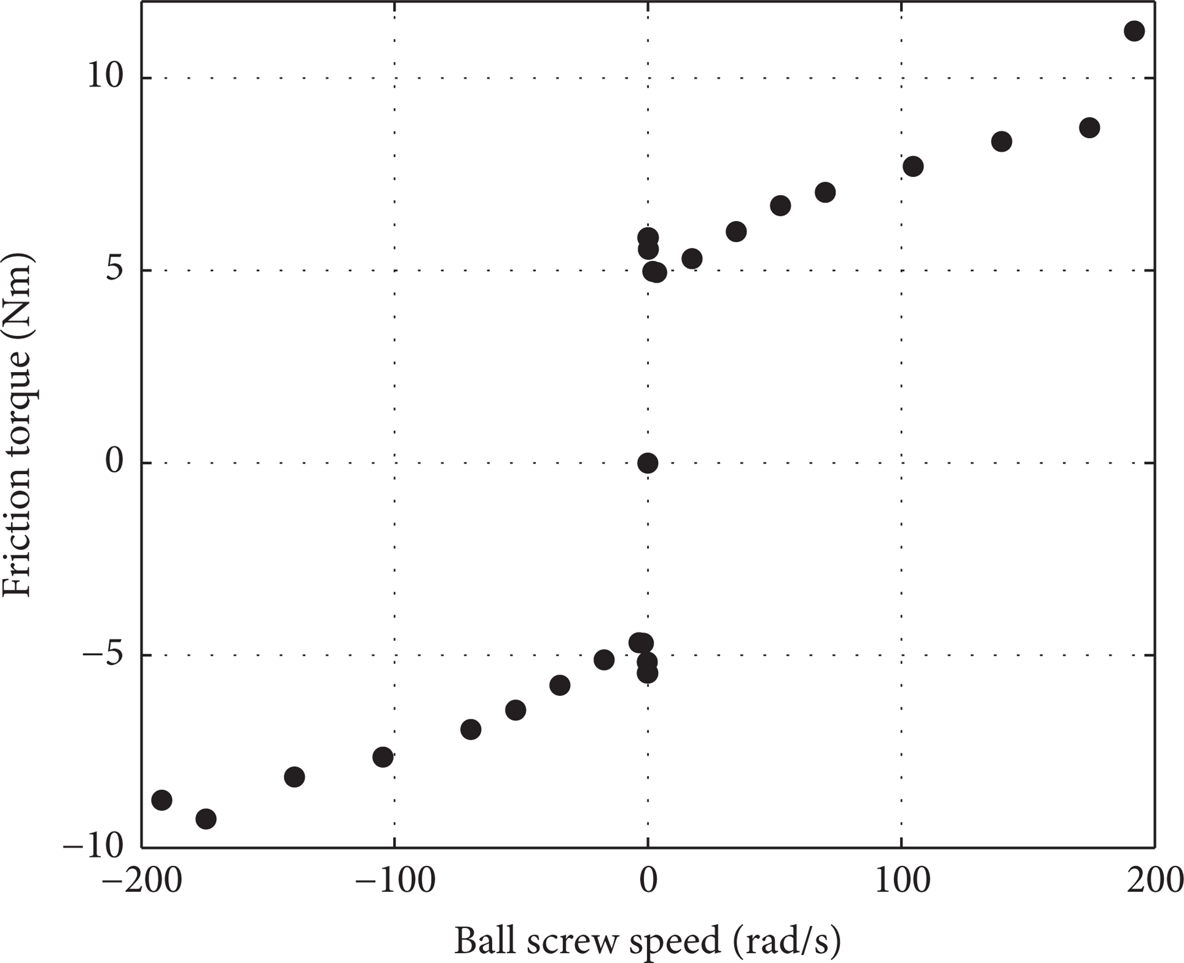
Friction on ball screw versus ball screw speed.

6. Model Validation

The model validation consisted in a comparison between the real system and the simulated response in frequency and time domain by using all the equations gathered herein plus experimental tests.

By using the internal routine of the numerical controller, the actual frequency response of the system was plotted. Figure 7 shows the response to a command of 0.01 mm of amplitude and with middle stroke as mean value. In the same figure the simulated response may be seen. From the modal analysis a first mechanical frequency equal to 152 Hz was found. By analysing the actual response of the machine it may be seen that there is a mechanical frequency nearby the former. This means that the modal analysis and stiffness calculations were performed correctly, based on the model developed. The amplitude plot highlights that some of the dynamic aspects of the system were not captured: around the first mechanical frequency of the model the real system displays two natural frequencies. However, the overall match found is fully satisfactory, in particular within the bandwidth of the system.

Figure 7:

Experimental and simulated frequency response of the axis.

In Figure 8(a) a simulated and real position response to a particular motion profile is depicted. This command will be used as a reference later on. In Figure 8(b) the simulated and real motor torque are shown. These two figures show a good match in static and transient conditions.

Figure 8:

Real and simulated responses in time domain.

7. Results and Discussion

The model was used to evaluate the performance of the axis as a function of some characteristic properties. In particular the effect of the stiffness of the structural parts of the axis on its first natural frequency was considered. Later the influence of the main proportional gain k _v in the position loop on energy consumption, static position error, and response time was analysed.

By studying the modal deformation of the springs, it is possible to determine which of them most affect the value of the first natural frequency. Given a modal form, the larger the amplitude of the modal deformation, the greater the effect on the natural frequency. In Figure 9 the first modal deformations of the system Δ₁₂ ^T , Δ₂₃ ^T , Δ₀ ^A , Δ₁₂ ^A , and Δ₂₃ ^A are plotted. It becomes clear that the first natural frequency is more sensitive to a variation in the support stiffness k₀ ^A than to the other stiffness because the magnitude of the modal deformation associated with it at least doubles the others.

Figure 9:

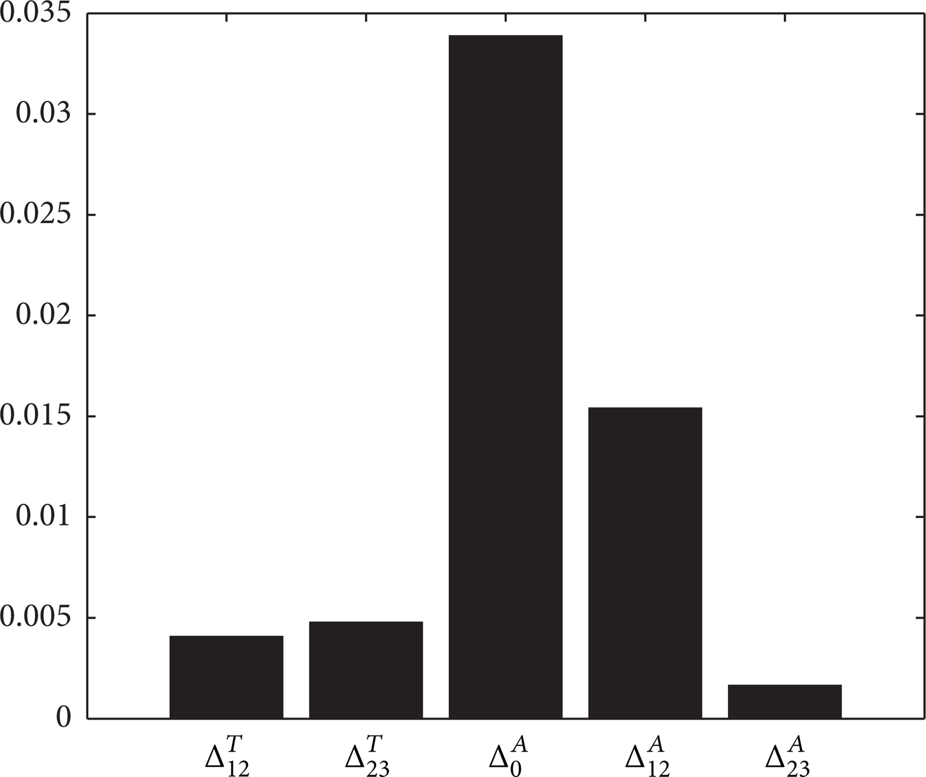
Amplitude of the first modal deformations.

To consolidate the above affirmation, Figure 10 shows the first frequency as a function of k₀ ^A which is ranging from 0.5 to 1.5 times its nominal value. The frequency changes considerably. This further proves the sensitivity to k₀ ^A .

Figure 10:

First mechanical frequency as function of k₀ ^A (ball nut in the middle of the axis stroke).

Another important aspect worth analysing is the effect of the proportional position gain k _v on the system response. Special attention was given to the energy consumption as a function of k _v . Taking as reference cycle the position command depicted in Figure 8(a), the total energy consumption was calculated for different values of k _v . It is worth mentioning that the time intervals in which the motor shaft is dragged by the screw are not considered. In those intervals the energy generated is simply dissipated. The static position error was also calculated for different values of the proportional gain of the position loop. Then, to evaluate the dynamic response of the axis, the response time τ was computed as the time the axis needs to travel from middle stroke to 99% of its end. Figure 11 shows how better performance in terms of axis precision and time response involves higher energy consumption per cycle.

Figure 11:

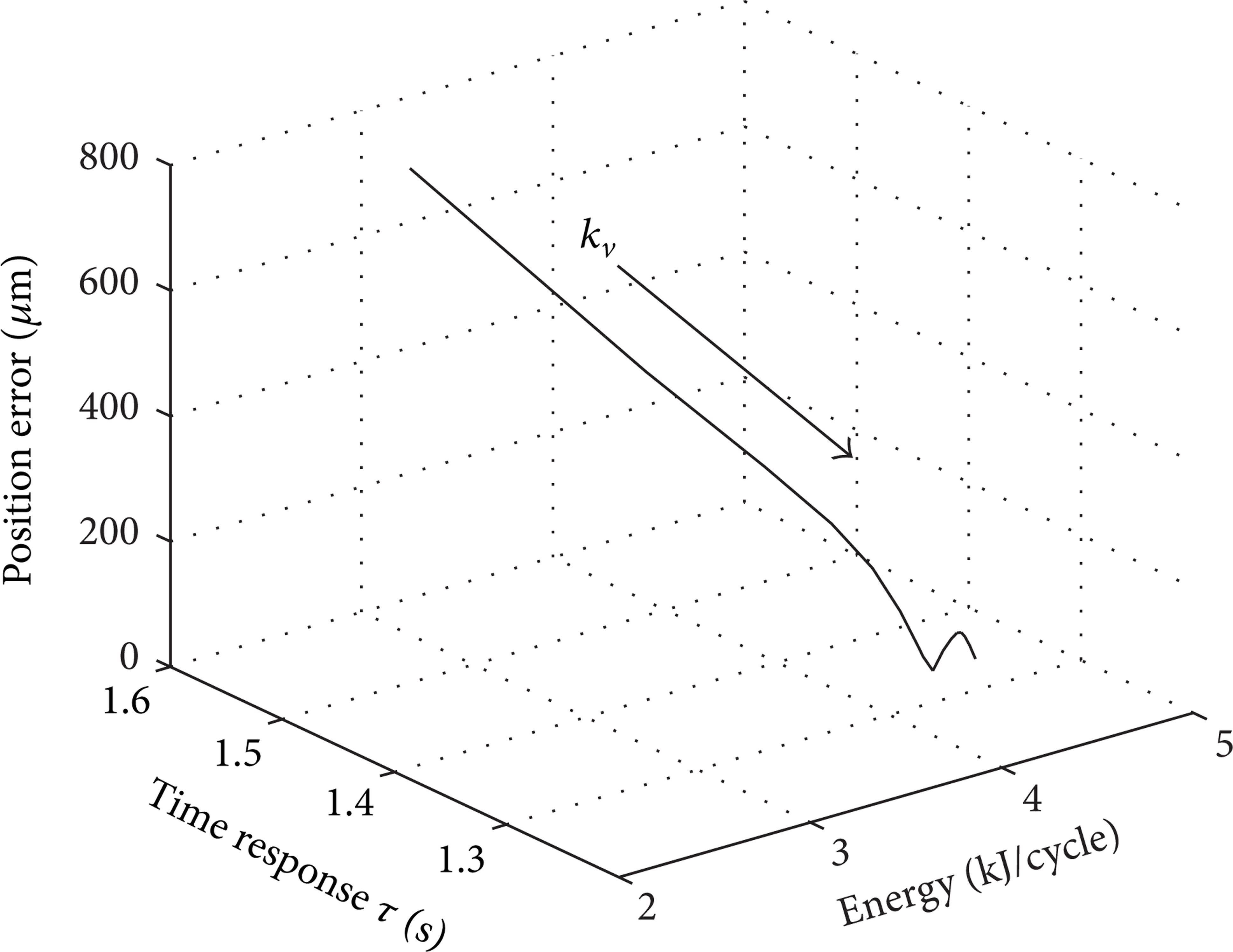
Energy consumption, position error, and time response for different values of k _v .

Energy consumption ener, static position error err, and time response τ have been analysed. All these parameters are important to evaluate the axis performance. By creating a cost function it is possible to evaluate different values of k _v in a complete way. If position error is seen as a cost, low energy consumption and settling time will decrease it. The former may be written as a cost function C(k _v ) given by

$C\left(k_v\right)=\frac{err\left(k_v\right)}{{err}_{\max }}-\frac{{ener}_{\min }}{ener\left(k_v\right)}-\mathrm{\hspace{0.17em}\hspace{0.17em}}\frac{{\tau }_{\min }}{\tau \left(k_v\right)}$

(22)

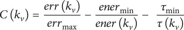
with 1 as the upper limit and −2 as the lower one. The proportional gain with the lowest value of C will theoretically be the optimal value under the point of view of this particular cost function. Table 1 summarizes Figure 11 and displays the cost function C.

Table 1:

Values of τ, static error, energy per cycle, and C as function of k _v .

k v (min−1)1	Error (µm)	τ (s)	Energy (KJ/cycle)	C (—)
625	758	1.548	2.948	−0.852
925	479	1.434	3.508	−1.127
1225	337	1.386	3.850	−1.272
1525	246	1.363	4.068	−1.366
1825	173	1.351	4.211	−1.448
2125	102	1.343	4.309	−1.531
2425	41	1.338	4.378	−1.604
2500	28	1.334	4.427	−1.620
2725	5	1.334	4.427	−1.648
3025	36	1.331	4.462	−1.603
3325	55	1.329	4.488	−1.577
3625	64	1.327	4.507	−1.563
3925	65	1.325	4.521	−1.561
4225	59	1.324	4.531	−1.569
4525	51	1.323	4.540	−1.579
4825	44	1.322	4.545	−1.588
5125	38	1.321	4.550	−1.595
5425	33	1.320	4.553	−1.602
5725	29	1.319	4.556	−1.608
6025	25	1.319	4.558	−1.613

1

Gain k _v is expressed in min⁻¹, the same unit used by the machine controller.

In Table 1 the optimal axis gain is highlighted. For k _v being equal to 2725 min⁻¹, the cost is the lowest, which means that an optimal error-energy-time combination corresponds to this value.

8. Conclusions

The work showed a method to analyse the sensitivity of the performance of a servoaxis of a tool machine to some main design parameters.

The result is obtained by developing a lumped parameter of the servoaxis that considers the deformability of its mechanical parts as well as their damping properties.

A schematization that mapped lumped stiffness parameters onto physical components was proposed. This made it possible to compute reliable stiffness values using catalogues when disposable and analytical or numerical computation technique for unknown components.

The model of the system was validated by comparison with data obtained by the tests of a real servoaxis.

A first result showed that the first mechanical frequency of the system is strongly influenced by the stiffness of the support of the axis, while the stiffness of the other components shows lower importance.

A second analysis regards the effect of the proportional gain; a criterion to identify an optimal value by considering precision, velocity, and energy consumption was formulated. The analysis put in evidence that precision is more sensitive to the axis gain than energy consumption and positioning time.

The method used to model the servoaxis showed itself to allow a reliable model to be developed and the developed model could be used to provide machine designer with information about acceptable stiffness values for the components of the servoaxis according to precision and frequency response requirements.

Conflict of Interests

The authors declare that there is no conflict of interests regarding the publication of this paper.