Sage Journals: Discover world-class research

Abstract

A wireless sensor network (WSN) consists of hundreds or thousands of sensor nodes organized in an ad hoc manner to achieve a predefined goal. Although WSNs have limitations in terms of memory and processors, the main constraint that makes WSNs different from traditional networks is the battery problem which limits the lifetime of a network. Different approaches are proposed in the literature for improving the network lifetime, including data aggregation, energy efficient routing schemes, and MAC protocols. Sink node mobility is also an effective approach for improving the network lifetime. In this paper, we investigate controlled sink node mobility and present a set of algorithms for deciding where and when to move a sink node to improve network lifetime. Moreover, we give a load-balanced topology construction algorithm as another component of our solution. We did extensive simulation experiments to evaluate the performance of the components of our mobility scheme and to compare our solution with static case and random movement strategy. The results show that our algorithms are effective in improving network lifetime and provide significantly better lifetime compared to static sink case and random movement strategy.

1. Introduction

The emergence of tiny sensor nodes as a result of advances in microelectromechanical systems has enabled wireless sensor networks (WSNs). A typical sensor node has generally an irreplaceable limited-capacity battery and therefore consuming the least amount of energy is the most critical criterion when designing any sensor network-related protocol. Since energy is the most precious resource, and in most of the applications replacing the batteries is very hard or impractical efficiently utilizing both node's and the total energy of the network is very important for a given task.

Several approaches are used in literature to minimize energy consumption in wireless sensor networks and improve network lifetime. Some of these approaches are adjusting transmit power, developing energy-efficient MAC or routing protocols, minimizing the number of messages traveling in the network, and putting some sensor nodes into sleep mode and using only a necessary set of nodes for sensing and communication.

Making the sink node mobile is another approach for improving the lifetime of WSNs. Sink node collects the incoming data from sensor nodes and when data aggregation is not used, each sensor node not only transmits its own packet to the sink, but also relays the packets of its children. Since most of the time a tree topology rooted at the sink is used to collect data, all packets are delivered to the sink node via its first-hop neighbors. As seen in Figure 1, this situation causes these nodes to deplete their energy faster than the other nodes in the network. Therefore, the main motivation behind sink mobility is to change these neighboring nodes periodically by moving the sink to different locations. A node that was a neighbor of the sink in a round and therefore had a large packet load should have a smaller packet load in the next round. This way the neighbor role is delegated fairly among all sensor nodes. In this way, on the average all nodes would have a nearly equal cumulative packet load and remaining energy levels at an arbitrary time.

Figure 1

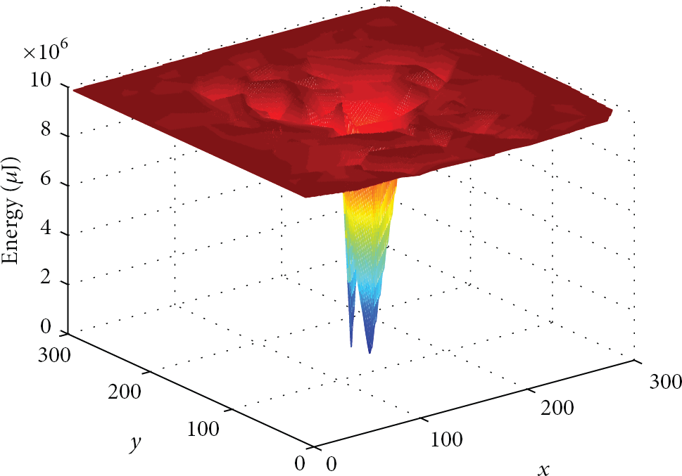
Energy map of a static sink after the first node death.

A sink mobility scheme has to address the issues of when and where to move the sink mode so that energy is consumed efficiently and in a balanced manner. Sink will stay at a point for a while and collects the data. Then it will move to a new location and will continue collecting data at that location. The time duration during which the sink stays at a fixed location is called sojourn time (or round duration) in this paper. The location where a sink stays to collect data for while is also called anchor point, migration point, or sink site. A given mobility scheme needs to also specify, which network parameters should be used to regulate this operation.

In this paper, we propose a set of algorithms for different aspects of the sink mobility problem in wireless sensor networks. We propose two sink-site determination algorithms. Additionally, we present an energy-efficient topology construction algorithm for improving the network lifetime. These issues have not been addressed together in most of the previous studies. Our simulation results show that the proposed algorithms perform better than other comparable methods and improve the network lifetime significantly.

The rest of the paper is organized as follows. In Section 2, related work about the sink mobility problem in wireless sensor networks is summarized and discussed. Section 3 describes our approach and algorithms. Results of our simulation experiments are presented in Section 4. Finally, Section 5 concludes the paper and gives future research directions.

2. Related Work

Since energy is the most precious resource in a sensor network, it should be carefully taken into consideration in any algorithm or approach related to sensor network design and operation. The studies targeting energy efficiency and network lifetime improvement in WSNs generally attack the problem in physical layer (power control [1, 2]), in data link layer (MAC protocols [3, 4]), in network layer (routing [5, 6]), or in application layer (topology control [7, 8], data gathering and aggregation [9–11], clustering [12, 13], and sleep scheduling [14]). Most of the papers deal with one of the aspects that lie only in one layer, whereas some other works [15, 16] use cross-layer design where different issues related to more than one layer are taken into consideration in order to maximize network lifetime.

Sink mobility approaches can be classified into two categories according to the moving strategy used: uncontrolled (random) and controlled [17]. In uncontrolled mobility, a third tier is used in the network, in which mobile agents (MULEs: mobile ubiquitous LAN extensions) are deployed between access points (base stations) and sensor nodes in order to collect data from sensor nodes when they get in contact, buffer the data, and finally transmit the data to the sink [18]. It is called uncontrolled, since movement is random and MULEs (for instance vehicles) move according to their needs and only exchange data if they encounter any node as a result of their movement [18].

The main motivation behind use of MULEs is to reduce transmission energy cost by using single-hop communication between a MULE and a sensor node, instead of the more expensive multihop communication traveling a long distance between the sink and a sensor node. Since communication is the most energy consuming part in network operations, this approach effectively increases network lifetime. However, since the arriving time of a MULE near a sensor node is not known a priori, two important problems emerge: large buffer size needed at nodes and large data latency. There is a trade-off between latency and energy consumption. If the application is delay tolerant, uncontrolled sink mobility becomes a good alternative. Packet losses need also to be considered if nodes do not have large enough buffers that can store the packets generated between two consecutive visits of a MULE.

In controlled mobility, sink is moved depending on network conditions (like current energy map, node density in the regions, etc.). Currently, there are three main approaches used in controlled mobility [19]. In first and mostly used one, the sink moves among the nodes and collects data without any additional entity (which is also the case in this work). In the second approach, mobile relays are used as forwarding agents, like MULEs but in a controlled manner, for communication between sensor nodes and the base station [20]. In the third approach, sensor nodes themselves are mobile [21]. Generally, sink node or relay nodes are assumed to have abundant energy resources so they do not deplete their energy during the network lifetime. Therefore it is expected that mobility of these types of nodes does not adversely affect the network lifetime. However, for sensor nodes this is not the case. As it was mentioned before, sensor nodes have very limited energy resources, which should not be wasted for mobility, topology reconstruction, and so forth, unless it is certainly necessary. That is why the first two approaches appear to be more promising for energy efficiency and longer network lifetime [19].

Choosing the appropriate scheme completely depends on the application the WSN will be used for. If we can tolerate data latency and some possible packet losses and/or we have relatively small deployment area and MULEs travel quite fast in that area, then it will be important to use data MULEs for communication in order to effectively reduce the energy consumption. However, if we have a critical application (which is our assumption in this work) that is intolerant to latency or packet losses, like earthquakes, fire detection, or battlefield surveillance, then controlled mobility (via either relays or sink) node becomes crucial. In this work, we focus on and propose algorithms for controlled sink mobility scenario.

Sink mobility differs from other approaches to save energy in the way it considers the resulting energy consumption behavior in the network. Most strategies other than sink mobility aim to minimize either average, or maximum energy consumption by using an appropriate technique; however, neither average nor maximum energy consumption based strategies consider current energy status of a node [23]. That is why they cannot avoid the nodes whose batteries are close to depletion. Unlike these approaches, in (controlled) sink mobility, current remaining energy values of sensor nodes are taken into consideration, and this helps to extend the lifetime of nodes as much as possible. This brings a serious advantage in the case where network lifetime is defined as the time passed until the first node depletes all its energy, which is commonly used definition in the literature.

Various studies deal with issues regarding sink mobility. Mobility and routing are considered together in [24]. The authors present a framework for investigating sink mobility and routing problem together in order to maximize network lifetime (MNL). They model MNL problem as a mixed integer linear programming formulation and prove its NP hardness involving multiple mobile sinks. Single sink and multiple sinks cases are investigated separately. An efficient primal-dual algorithm is given for the single sink case and it is approximated to multiple sinks case. Sink locations are constrained (to finite locations) here, as well. Numerical experiments are performed to measure the primal-dual algorithm's performance in terms of network lifetime and pause time distribution. Achievable lifetime between mobile sink and static sink (at its optimal position) is compared in line, ring, and grid networks for varying number of nodes. The difference between two approaches increases in grid networks and becomes 555% when the number of nodes is 289.

A work more similar to ours is presented in [25]. The authors present two complementary algorithms for solving the sink mobility and routing problems together. One is the scheduling algorithm, which determines the duration the sink node can stay at each candidate sink site, and the other is the routing algorithm, which finds the most energy-efficient paths for each packet from a sensor node to the sink. A linear programming (LP) formulation is given that maximizes the network lifetime, the sum of sink sojourn times at all possible locations, subject to some constraints, and then compares mobile and static sink approaches with different routing schemes. In the simulations, there are two scenarios, including just four (centers of four subsquares) and five (corners and center) different sink sites, respectively. Experiments are done and compared between static and mobile sink approaches via adding the routing parameter; however, there is no comparison between the proposed mobility model and any other mobile strategy in the paper.

In [26], authors present an LP formulation to maximize the overall network lifetime (the sum of sojourn times of the sink) instead of minimizing the energy consumptions at the sensors. It is assumed that nodes are deployed to a $L x L$ grid such that, $n = L^{2}$ , where n is the number of nodes. The authors evaluate the performance of the proposed LP model for various network sizes and compare their performance with static sink case and improve network lifetime up to almost five times. Their proposed solution results in a fair balancing of energy consumption among the sensor nodes. They can, however, measure the performance of the proposed model up to $256$ nodes due to LP constraints and restrict the network deployment to put sensor nodes to the corners of the grids.

A detailed work about controlled sink mobility is presented in [19]. The authors present a centralized mixed integer linear programming (MILP) model that determines sojourn times and the order of visits to sink sites. Moreover, a fully distributed and localized heuristic (GMRE) is developed as a solution to the problem. The deployment area is divided into grids and the corners of these grids are determined as the sink sites. The MILP formulation aims to maximize total sojourn time, as in [25], subject to some constraints. They evaluate the performance of MILP, GMRE, random movement (RM), and static sink approaches with different node deployment strategies and constraints on the sink movements. MILP and GMRE give better results than the others. Moreover, MILP performs between 30% and 50% better than GMRE.

Basagni et al. investigate the lifetime maximization problem for multiple mobile sinks case as well [27]. They first present a mixed integer linear programming (MILP) model to give a provable upper bound on the lifetime of the WSNs. The output of LP is used to provide a polynomial time centralized heuristic. Lastly, a distributed heuristic is proposed for coordinating the motion of the multiple sinks. The simulation results show that proposed schemes improve lifetime significantly compared to the cases of static sink and random sink mobility.

A distributed algorithm, mostly using local information, for delay-tolerant wireless sensor networks is given in [28]. The authors investigate the problem of maximizing the number of tours (T), such that each tour takes D (maximum delay tolerance) time units (lifetime becomes $T \cdot D$ ). They first formulate the problem, decompose it by Lagrangian relaxation, and give algorithms for these subproblems. Finally, the algorithms are combined into the main algorithm. The authors give an analysis to show that their algorithm converges to the optimal solution and verify it via simulations.

3. Proposed Algorithms

3.1. Sink-Site Determination

The main motivation behind sink-site determination (SSD) algorithms is to decrease candidate migration points in the deployment area to minimize the time needed to determine which sink site to visit next after the sojourn time at the current sink site expires. In some scenarios, sensor nodes are deployed to areas where some points may be inaccessible or very difficult to access, and thus the sink may not be able to reach them. These reasons force us to choose sink sites before the network starts operating.

In the literature, such as in [19, 25], the deployment area is divided into grids and sink sites are determined as the corners of those grids without any computation. However, in nonregular deployment, it would be better to determine the sites by considering the deployment characteristics and neighborhood information of nodes. We propose two sink-site determination algorithms in which network structure and conditions (deployment, neighborhood relationships, etc.) are taken into consideration.

3.1.1. Neighborhood-Based Sink-Site Determination Algorithm

Sometimes it can be difficult to know the exact boundaries of the deployment area and the coordinates of each sensor node in the region. In such cases, neighborhood information of the nodes can be used for determining candidate sink positions. If we are given n nodes and their neighborhood information, then our aim is to choose q nodes from the list such that the union of the neighbors of these selected nodes covers all the nodes in the area. This process is quite similar to finding a dominating set for a graph $G = (V, E)$ , which is defined as every vertex not in the dominating set D is adjacent to at least one vertex in D [29]. The dominating set problem is a special instance of the set covering problem and it is NP-complete [30] (the decision version of set covering is NP-complete, and the optimization version of set cover is NP-hard since it generalizes the NP complete vertex-cover problem [31]).

In Algorithm 1, we give a heuristic algorithm for dealing with the dominating set problem in this context. Here, first all neighbors broadcast a message in order to collect their neighborhood information. Then, this information is sent to the sink to determine possible sites. The sink node sorts the nodes in descending order with respect to their number of neighbors. Then the algorithm takes the coordinate of the node (a contributed node) with the most number of neighbors in the beginning and put those neighbors to the current neighbor list. After this step, the algorithm maintains the list of covered and uncovered nodes at each step. After first contributed node is chosen, its neighbors are saved in $c o v n$ (covered nodes) list. The $u n c o v n$ (uncovered nodes) list is simply calculated via taking set difference of universal set (all nodes) and $c o v n$ list. After initialization of those lists, the node that has the maximum number of common elements with $u n c o v n$ is chosen as the next contributed node. Then its neighbors are added to $c o v n$ list, and $u n c o v n$ list is updated. This iteration continues until $u n c o v n$ list becomes empty (i.e., $c o v n$ equals universal list). The algorithm's complexity is $O (n^{2})$ in the worst case.

Algorithm 1: Neighborhood-based SSD algorithm.

(1) procedure NBSSD

(2) for $i \leftarrow 1, N$ do

(3) $n g (i) \leftarrow i d_{r}$ ⊳ $i d_{r}$ : node id in each received msg

(4) $n s (i) \leftarrow s i z e (n g (i))$ ⊳ get size of each list

(5) end for

(6) $n s i \leftarrow s o r t (n s)$ ⊳ return indices of reverse sorted $n s$

(7) $i n d \leftarrow 1$

(8) $c n (i n d) \leftarrow n s i (1)$ ⊳ get first contributed node id

(9) $c o v n \leftarrow n g (c n (i n d))$ ⊳ get neighbor info of first cn

(10) $u n c o v n \leftarrow n o d e s - {c o v n}$ ⊳ uncovered nodes = all − covered

(11) $i n d \leftarrow i n d + 1$

(12) while $u n c o v n \neq ϕ$ do ⊳ run until all nodes are covered

(13) for $j \leftarrow 1, s i z e (n s i)$ do

(14) $c e (j) \leftarrow s i z e (n g (n s i (j)) \cap u n c o v n)$

(15) end for

(16) $c x \leftarrow \max (c e)$ ⊳ get the most intersected

(17) $c n (i n d) \leftarrow n s i (c x)$

(18) $i n d \leftarrow i n d + 1$

(19) $c o v n \leftarrow c o v n \cup n g (c n (i n d))$

(20) $u n c o v n \leftarrow n o d e s - {c o v n}$

(21) end while

(22) for $i \leftarrow 1, s i z e (c o v n)$ do

(23) $mp (i) \leftarrow c x y (c n (i))$ ⊳ migration points as coordinates of $c n$ s

(24) end for

(25) return $mp$

(26) end procedure

3.1.2. Coordinate-Based Sink-Site Determination Algorithm

It is possible to group nodes using their coordinate values (if they are known) on the sink. In the coordinate-based sink-site determination algorithm, we divide the deployment area into squares such that each one's length is equal to the transmission range. That enables us to group (cluster) nodes that can be a sink's neighbors in any round and compare their energy levels and decide which subarea to move to in the next round. The number of areas dynamically changes according to the transmission range values. The distance between any two neighbor sink sites is R, where R is the maximum transmission range. Each sink site is ideally placed at the center of a subsquare area. If area center is not accessible (because of an obstacle for instance), this can only cause some nodes not to be one-hop neighbor of the sink but to be two hops away from it.

Number of points in each subsquare should be known in order to calculate the threshold value ( $n / s$ ) and eliminate sparse areas in Algorithm 2. Given N points in the plane, how many of them lie in a given region (report the points ( $x_{i}, y_{i}$ ) such that $l_{x} \leq x_{i} \leq r_{x}$ , $l_{y} \leq y_{i} \leq r_{y}$ ) is a typical range searching or geometric search problem. Different data structures (k-d trees, range trees) can be used for answering this kind of queries [22]. K-d trees have $O (n)$ , $O (n \log n)$ , and $O (\sqrt{n} + k)$ complexity for storage, preprocessing, and querying operations, respectively (n: total number of points, k: number of reported points). Querying time can be reduced to $O (\log^{2} n + k)$ with range trees when paying the price of increase in storage from $O (n)$ to $O (n \log n)$ . We can use range trees here to query the number of points falling into each subsquare.

Algorithm 2: Coordinate-based SSD algorithm.

(1) procedure CBSSDA( $c x y, R$ ) ⊳ $c x y$ : node coordinates, R: tx range

(2) $s \leftarrow (L / R)^{2}$ ⊳s: # of sub-squares

(3) $i n d \leftarrow 1$

(4) for $i \leftarrow 1, s$ do

(5) $c mp (i) \leftarrow (x c_{i}, y c_{i})$ ⊳ coordinates of each subsquare center State

$s x y (i) \leftarrow [l x_{i}, r x_{i}] x [l y_{i}, r y_{i}]$ ⊳ subsquare coordinates in the plane

(6) end for

(7) $t \leftarrow n / s$ ⊳ set threshold

(8) $t r e e \leftarrow b u i l d 2 d r a n g e t r e e (c x y)$ ⊳ building range tree function in [22]

(9) $i n d \leftarrow 1$

(10) for $i \leftarrow 1, s i z e (c mp)$ do

(11) $n s (i) \leftarrow 2 d r a n g e q u e r y (t r e e, s x y)$ ⊳ # of nodes fall into sub-square i

(12) if $n s (i) \geq t$ then ⊳ accessible and density ≥ threshold

(13) $mp (i n d) = c mp (i)$

(14) $i n d \leftarrow i n d + 1$

(15) end if

(16) end for

(17) return $c mp$

(18) end procedure

The detailed algorithm is given in Algorithm 2. After determining the centers of each subsquare, range tree is built. Number of points in each subsquare is determined querying the tree for its coordinates in the plane. Sparse areas are eliminated if their density is below the threshold, where the threshold is determined by dividing the number of nodes by the number of subsquares. If there are many sparse areas this will decrease the number of candidate migration points. However, this situation does not cause any disconnectivity, since those areas will be connected to the sink via multihop topology.

Since each node's coordinate is known by the sink node, the area does not have to be regularly divided into squares in order to use this algorithm. The sink node can choose the node that has the minimum (x, y) pair and assume that it is located on the lower-left corner of the imaginary subsquare. Then it chooses the center of this subsquare as the candidate migration point and continues this operation until all the nodes in the area are covered. Since the algorithm iterates two times over the number of subsquares (s), its complexity is $O (n \log n)$ for range tree construction and $O (s (\log^{2} n + k))$ , where s is calculated as $(L / R)^{2}$ (L: side length and R: transmission range) and k is the number of reported points.

A dynamic sink-site selection algorithm (either neighborhood- or coordinate-based) enables us to eliminate areas on inaccessible terrains.

3.2. Sojourn Time and Movement Criterion

After candidate sink sites are determined, the sink node moves to the densest point of the area (first migration point) and the routing topology (i.e., the tree) is constructed (either via simple broadcasting or an intelligent topology construction mechanism as in Algorithm 4). The sink determines the remaining energy values of its neighbors to learn the minimum energy levels of its neighbors before packets arrive. Since energy levels are piggybacked in each packet, the sink node can compare the current minimum energy value and the initial one. If the difference between them is one unit or more, then the sink node initiates the process of determining the location to move in the next round. Sojourn time of the sink node expires when energy change of any node becomes greater than $1 / L$ of its initial energy. Some applications require a minimum sojourn time on a site in order to ensure data quality. For these cases, we can use a parameter, $t_{\min}$ (as in [19]), which is the minimum time that a sink node should stay on the current site.

Such a dynamic approach is more advantageous than a static case where a fixed number of rounds are used. For instance, a sink can immediately move to another site if a sink neighbor has a tremendous packet load and rapidly consumes its energy. However, a fixed-round approach will wait until the required number of rounds is completed, which may cause a node to die.

If the sojourn time expires (either exceeds $t_{\min}$ or a change in energy level occurs), the sink examines the minimum remaining energy value in each candidate migration point using the recent information piggybacked in the last received packets. Then it moves to the point where the minimum remaining energy level is maximum among the sites that have not been visited yet (visit added max-min approach (VMM)). When we say “have not been visited”, we mean that a site cannot be visited until the sink has moved to all of the candidate migration points once. After all visits have been completed, the visited flag will be set to zero for all of the sites and they all become available to be visited again.

The motivation behind this approach is the following: if we use just the max-min approach, then we may get stuck to a single local maximum and unable to focus on the general picture. In other words, when we are only interested in the energy dimension of the problem, then we can only ping pong among a few sink sites that have similar packet load patterns (if a deterministic topology construction algorithm is used, as in the next section). However, if we visit different sites, then we can achieve a more uniform packet load distribution. Therefore, the visit added max-min (VMM) approach, which is summarized in Algorithm 3, corresponds to visiting possible sink sites in the order of which the maximum of the minimum energy values in the sites takes precedence. Since the algorithm iterates over the number of migration points (m) and calculates minimum energy among the nodes on each site, its complexity is $O (m n)$ (where n is the number of nodes) in the worst case.

Algorithm 3: Migration algorithm.

(1) procedure MA( $mp, R$ ) ⊳ $mp$ : migration points, R: tx range

(2) $n v l \leftarrow mp$ ⊳ set not visited list

(3) $c x y_{s} \leftarrow mp (1)$ ⊳ sink goes to first migration point

(4) $n v l \leftarrow n v l - {1}$

(5) while $e > 0$ do ⊳ any node's energy is not depleted

(6) $e_{i} = e_{i} - c t x_{i} + c r_{i}$ ⊳ transmission and receive costs

(7) if $e l_{i + 1} - e l_{i} > 0$ then ⊳ if energy level change occurs

(8) for $i \leftarrow 1, s i z e (n v l)$ do

(9) $n g (i) \leftarrow d i s t (c x y, mp (i))$ ⊳ nodes in tx range of $mp (i)$

(10) $e n l (i) \leftarrow \min (e (n g (i)))$ ⊳ get min energy from $mp (i)$

(11) end for

(12) $i n d \leftarrow \max (e n l)$

(13) $n s \leftarrow n v l (i n d)$ ⊳ set next site

(14) $n v l \leftarrow n v l - {i n d}$

(15) if $n v l = ϕ$ then

(16) $n v l \leftarrow mp$

(17) end if

(18) $c x y_{s} \leftarrow mp (i n d)$ ⊳ sink moves to next migration point

(19) end if

(20) end while

(21) end procedure

Algorithm 4: Load-balanced topology construction algorithm.

(1) procedure LBTCA ⊳ initialization of sink node

(2) $ll (0) \leftarrow 0$ ⊳ logical level (hop distance to sink)

(3) $pl (0) \leftarrow N U L L$ ⊳ parent list (all ids from upper level)

(4) for $i \leftarrow 1, N$ do

(5) $ll (i) \leftarrow - 1$

(6) $pl (i) \leftarrow - 1$

(7) end for

(8) $brcs (0,0)$ ⊳ sink broadcasts its id and logical level

(9) while $ll < 0$ do ⊳ broadcast untill all nodes are reached

(10) if $rc v_{i} (j)$ then ⊳ if node i receives a msg from j

(11) if $l l_{i} < 0$ then ⊳ this is the first msg received

(12) $l l_{i} \leftarrow l l_{j} + 1$

(13) $brcs (i, l l_{i})$

(14) end if

(15) $pl (i) \leftarrow pl (i) \cup j$ ⊳ updates parent list

(16) end if

(17) end while

(18) $ml \leftarrow \max (ll)$ ⊳ get max level from leaves

(19) for $l k \leftarrow ml, 1$ do ⊳ start from leaves

(20) $c n l \leftarrow f i n d (l l, k)$ ⊳ find nodes have level of k

(21) $s pl \leftarrow s o r t (c n l, pl)$ ⊳ sort nodes according to # of parents

(22) for $i \leftarrow 1, s i z e (c n l)$ do

(23) if $s i z e (s p l_{i}) = 1$ then ⊳ assign unique option as parent

(24) $n o d e s  (i) \cdot p a r e n t \leftarrow s p l_{i} (1)$

(25) else

(26) for $j \leftarrow 1, s i z e (s p l_{i})$ do

(27) $r (j) \leftarrow e_{j} / cp l^{2}$

(28) end for

(29) $i n d \leftarrow \max (r)$

(30) $n o d e s  (i) \cdot p a r e n t \leftarrow s p l_{i} (i n d)$ ;

(31) end if

(32) $n o d e s  (p a r e n t_{i}) \cdot pl + = n o d e s  (i) \cdot pl$ ⊳ updates packet loads

(33) end for

(34) end for

(35) end procedure

3.3. Load-Balanced Topology Construction Algorithm

Repositioning the sink node requires a topology reconstruction cost, which is the main drawback of a mobility scheme. An energy-efficient topology construction algorithm is an important component of such a mobility scheme to reduce this repeating cost. A typical broadcast mechanism is used for constructing a tree-based routing topology as the basic solution.

In this mechanism, after the mobile sink moves to its initial location, it broadcasts messages in order to construct the topology from top to bottom. Each node that receives the message (i.e., the nodes in the transmission range of the sender) rebroadcasts the message after putting their ID as the parent ID in a field of the packet. Each node that receives the broadcast packet saves the parent ID. However, in the approach above, current energy levels of the nodes are not taken into consideration. An algorithm that considers the current energy levels and packet load of the nodes should yield a better network lifetime.

Algorithm 4 gives a balanced tree-based topology construction mechanism. Sink's neighbors are in the first level in the logical tree, the neighbors of its neighbors are in the second level, and so on. For each node in level l, if a neighbor node is in the logical level $l - 1$ , it becomes a candidate parent and its ID is put into the parent list. After calculating these values, the algorithm starts to run in the last logical level of the tree, namely, the leaves. The nodes in the last level of the tree are sorted according to the number of candidate parents, in ascending order. The main motivation behind sorting the nodes is to give priority to the nodes with fewer options. In this way, when we come to nodes with more options, that is, nodes with updated packet loads, a better decision can be made.

If a node has only one parent in its list, that node is designated as the parent node and its packet load is increased by the packet load of the child. If a node has more than one candidate parent, the ratio of $e / (cpl)^{2}$ (where e is current energy level and $cpl$ current packet load, resp.) is calculated for each candidate. This ratio helps the child to choose more advantageous one (has sufficient energy compared to current packet load) among possible alternatives. For instance, let us assume there are two parent alternatives, which have (4, 2) and (10, 3) as (energy level, current packet load) values, respectively. The algorithm selects the latter one, even if it has more packet load, because its ratio is bigger than the other. Since the algorithm is run from bottom to top, the packet load of the most critical nodes (i.e., sink neighbors) can be determined using the full information of the nodes below.

The algorithm consists of two main for loops. The first loop's complexity is $O (n)$ . The second loop iterates for each candidate parent of each node in each level in the tree. The outer two loops iterate over all the nodes in the area (iteration is over the nodes level by level). In the worst case, a node can access all nodes in one hop; therefore its number of neighbors can be equal to $n - 1$ . In this case, we have two loops which iterate for n and $n - 1$ nodes, respectively, which yields $O (n^{2})$ complexity.

4. Simulation Results

In this section, we present the results of the experiments that evaluate the performance of the algorithms presented in the previous part. We use MATLAB as the simulation environment. Simulations are done to observe the performance of the sink-site determination algorithms, movement criteria, and the topology reconstruction algorithm. Different metrics (network lifetime, packet latency) are examined for each category. We compare our movement scheme not only with the static sink case but also with random movement, where the sink randomly moves between predetermined sites after the sojourn time expires.

4.1. Scenarios and Parameters of the Simulation

Sensor networks generated in the simulation have N static sensor nodes and a single mobile base station (mobile sink). Those nodes are deployed to a region of interest in random and uniform manner. Square areas are used in the simulations, which are generally either $300 \times 300$ m² or $400 \times 400$ m². After the mobile sink moves to its initial location, it broadcasts messages in order to construct a tree-based multihop routing topology (sensors can reach to sink via their neighbors) from top to bottom (if a balanced tree-based topology construction is not used). After the topology construction, nodes start sensing the environment. There is a constant packet generation rate $Q_{i}$ (1 packet/s) for each sensor node $i \in N$ . In this work, we define the network lifetime as the period of time until the first node dies, which is a commonly used definition in the literature, and data latency as average hop count of a packet destined to the sink (which also implies how many nodes relay the packet up until it is reached to the sink).

The energy model and the radio characteristics used in the simulations come from [32]. Transmission energy cost is related to the number of bits and the square of distance, whereas receive energy cost is related to the number of bits. In our simulations, this energy model is applied with 50 bytes of data packets and 20 bytes of control packets (for topology construction purposes). The radio dissipates $E_{elec}$ = 50 nJ/bit to run the transceiver circuitry and $ϵ_{amp}$ = 100 pJ/bit/ $m^{2}$ for the transmit amplifier to achieve an acceptable $E_{b} / E_{n}$ [32]. Each sensor node has energy of 10 J initially. If not stated otherwise, this energy is divided into 20 levels and represented in five bits, which are piggybacked onto the data packets.

We investigate the performance of the algorithms in three sections. First, we evaluate the two proposed sink-site selection methods with another three in the literature in terms of network lifetime and data latency. Next, experiments about the performance of different movement criteria (visit added maximum of minimums, random movement, and static sink) are done for given sink sites. Lastly, typical broadcast mechanism and load-balanced topology construction algorithms are compared while other network parameters are fixed.

4.2. Sink-Site Determination Experiments

Sink sites are determined to answer the question of where to move the base station during network operation. Sink-site determination is mostly done by assigning a set of predefined points to the area. Some existing approaches are summarized in Figure 2. Figures 2(a) and 2(b) give examples for the approaches used by Papadimitriou and Georgiadis. [25]. We call these two approaches P1 and P2. In P1, center points of four grids are chosen as sink sites, whereas P2 takes four corner points and the center of the big square (coordinates are given for a $100 \times 100$ m square). In the third approach, Figure 2(c), which comes from Basagni et al. [19], the area is divided into $3 \times 3$ or $5 \times 5$ grids, totally 16 or 36 subsquares, and the corner points of subsquares are taken as candidate migration points. We call the approach using $3 \times 3$ grids B1 and the approach using $5 \times 5$ grids B2. We compare the performance of our two sink-site determination approaches (neighborhood-based set covering heuristic (NB) and coordinate-based (CB)) with these four approaches (P1, P2, B1, and B2).

Figure 2

Different sink-site selection approaches.

As can be seen in Figure 3, both neighbor- and coordinate-based approaches perform better than the other four in terms of network lifetime. The CB approach is three times better than P2 for 500 nodes as well. When we look at Figure 4, it can be seen that although P1 has the lowest network lifetime of the five approaches, it has the best data latency (average hop count) because four different sites have been optimally placed in the center of the four grids. Although the NB and CB approaches have a 25% worse data latency than P1 (since latency is not the primary concern when determining the sites), they have up to 60% better network lifetimes and better data latency than the other three (P2, B1, and B2 choose the corner of the grids which increases the average hop count to the sink, which is defined as latency) in all cases as well.

Figure 3

Sink-site determination approaches: network lifetime comparison.

Figure 4

Sink-site determination approaches: data latency comparison.

4.3. Sink Mobility Experiments

In this section, we investigate movement patterns. Before going into detail, we give information about the general structure of the experiments. As the first step of our overall scheme, we choose one of the sink-site determination methods discussed in the previous section, either the coordinate-based determination or neighborhood-based determination algorithm. For the second step, the max-min approach, the visit-added max-min approach, or the random movement approach is chosen as a strategy when moving through migration points. In RM, when the sojourn time expires, the base station moves to the coordinate of a random sink site in the area. The static sink (STS) is used as a fourth approach. As its name implies, in this case, the sink does not move between points in the area but is placed at the center of the area, which is the point that maximizes the network lifetime [33]. In all approaches, if one of the neighbors of the sink loses one or more levels of energy (out of 20 levels, 5% of its whole energy), then the sink decides to move to another point (its sojourn time expires).

In the experiment, $t_{\min}$ (as in [19]) is the minimum time the base station must stay at its current site. After this time expires, the sink controls whether one energy level change (among L values) has occurred or not. If this is so, the sink decides to move; otherwise it remains where it is until the next decision time arrives. With a $t_{\min}$ value, it is possible to observe the effect of the sink mobility trend in the network. For small values of $t_{\min}$ , the sink becomes highly mobile, whereas for larger values of $t_{\min}$ it tends to stay longer on a site, thus demonstrating a low mobility pattern. Figure 5 shows the results of different approaches under $t_{\min}$ values between 50 and 250 simulation seconds. 400 nodes are randomly deployed to an area of $300 \times 300$ m and $t_{x}$ value of 30 m. The figure shows that VMM performs better than all other approaches. Network lifetime values of VMM increase up to a point (for $t_{\min} = 200$ , in this case) and then start to decrease again. If sink changes its location too frequently this will cause higher topology construction cost. If it stays too long, then it will not utilize the benefits (even load distribution of sink's neighbors) of mobility (lifetime will decrease). That is why we see first an increase following a decrease in the results.

Figure 5

Network lifetime for 400 nodes (SSD = DSH and $t_{x} = 30$ m).

Data latency values of the approaches can be seen in Figure 6. As it is seen, static sink has the lowest latency (since it is placed in the center of the area which is optimal and stays there at the end of the network lifetime) and random movement follows it (it tends to move the sink to the center of the area mostly). VMM has lower latency than MM, and this can be seen as an achievement, since latency is decreasing while the network lifetime is increasing at the same time. RM has lower latency than VMM, since VMM uses more intelligent approach and higher network lifetime. However, when time goes to infinity, on the average, RM visits each site for equal number of times and this balances number of hop counts to the sink.

Figure 6

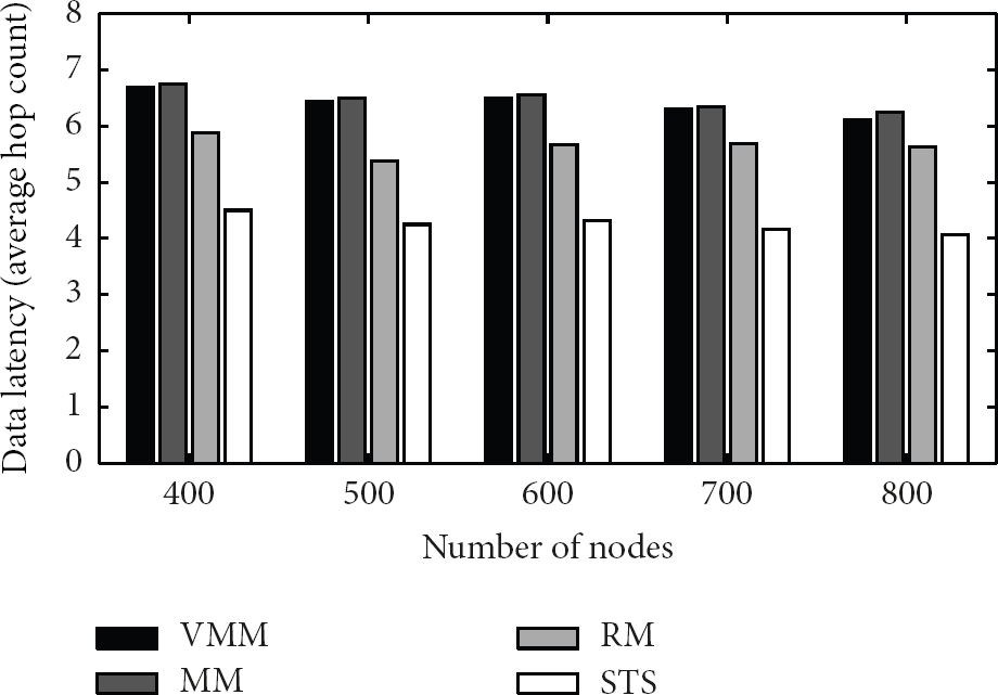
Data latency values for varying number of nodes (area side = 300 m and $t_{x} = 35$ m).

4.4. Different Network Topology Construction Mechanisms Experiments

In this section, two different topology construction algorithms are compared in terms of network lifetime and data latency. The first one uses a simple broadcast mechanism and the second uses the load-balanced approach, that is, Algorithm 4. In Figure 7, different numbers of nodes are deployed randomly to an area of $100 \times 100$ m with a transmission radius of 15 m. As can be seen from the figure, when the number of nodes increases, the load-balanced algorithm performs much better (100%) than the simple broadcast mechanism. Data latency experiments were also done, however, not shown here due to page limitations. Although the load-balanced algorithm achieves a nearly two times bigger network lifetime in some cases, it only has a 2.6% bigger average hop count value at most (this is intuitive because the load-balanced topology algorithm aims to distribute the load as uniformly as possible instead of using the shortest paths). That means the balanced tree topology construction approach significantly improves the network lifetime and causes only very low extra data latency overhead when doing that.

Figure 7

Network lifetime for different topology construction mechanisms (area side = 100 m and $t_{x} = 15$ m).

After examining different parts of the scheme, it would be reasonable here to see the overall performance of the proposed algorithms together. In this experiment, we compare two different mobility schemes with different properties. The first one uses the coordinate-based sink-site determination algorithm, VMM, and the balanced tree-based construction algorithm for topology generation. The second method uses the grid-based sink-site determination algorithm, RM, and the simple broadcast mechanism for topology construction. 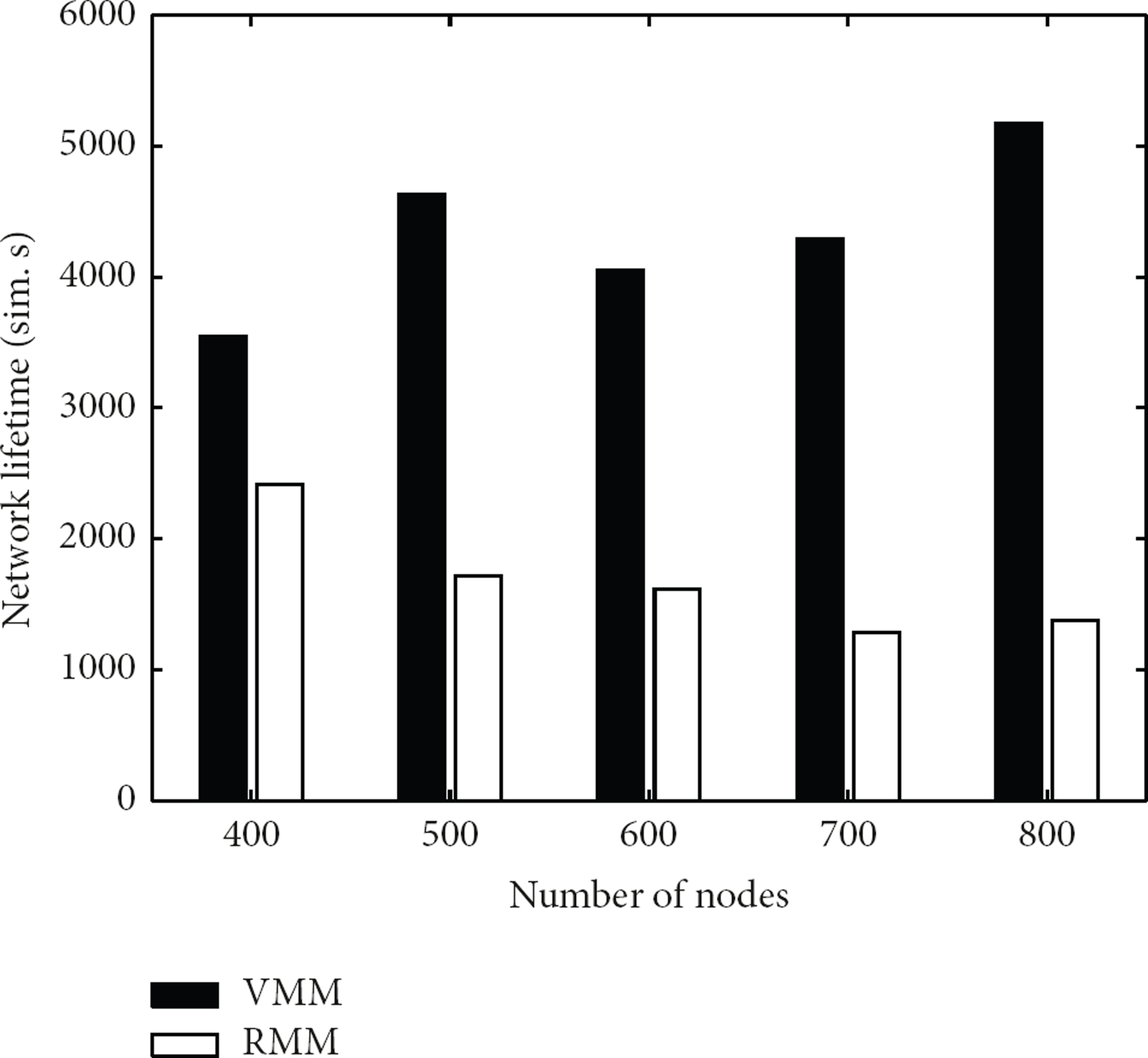In the experiment, a varying number of nodes are deployed to an area of $300 \times 300$ m² with a transmission range of 30 m. As seen in Figure 8, the network lifetime difference between these two approaches increases when the number of nodes increases. The VMM approach performs up to 3.5 times better than the random movement case, even though RM is also a mobility scheme. This brings an important improvement to the network lifetime when using different components of the scheme together.

Figure 8

Network lifetime performance of the entire scheme (area side = 300 m and $t_{x} = 30$ m).

5. Conclusion and Future Work

In this paper we investigate the controlled sink mobility problem to improve lifetime of wireless sensor networks. We deal with different components of the sink mobility problem. First, we propose two efficient sink-site determination algorithms, using neighborhood relationships and coordinates of nodes as inputs. Instead of using predefined time or round values, we also determine sojourn times using a dynamic approach. In order to choose the next site to visit, the sink node uses a visit-added max-min (VMM) approach. Unlike previous works, which used linear programming, there is no scalability problem in our approach. Moreover, a balanced tree topology construction algorithm is proposed instead of using a simple broadcast mechanism. In this algorithm, current energy levels of the nodes are taken into consideration, and packet loads are distributed, from bottom to top, using this information.

We compare the performance of our algorithms with different approaches via simulation experiments. Our sink-site determination algorithms perform better than the other four approaches from the literature. They also have lower data latency than three of the other approaches. Our VMM scheme gives better results than the random movement (RM) approach and the static sink (STS) case. Our energy-efficient topology construction algorithm performs better than the simple broadcasting mechanism in terms of network lifetime (for various node counts and transmission ranges), albeit introducing a very small extra latency overhead.

Although different components of the sink mobility problem are investigated in this study, there are still many issues to be investigated. In our work we assume nodes are randomly and uniformly deployed to the area. Different deployment strategies can also be tested and evaluated. Network lifetime definition is another point to be diversified. We define it as the time that passes until the first node exhausts its energy. There are other definitions that can be used and tested, such as the time until the percentage of messages received drops below a threshold.

Footnotes

Conflict of Interests

The authors declare that there is no conflict of interests regarding the publication of this paper.

References

Zongkai

Dasheng

Wenqing

Jianhua

Laganá

Gavrilova

M. L.

Kumar

Mun

Tan

C. J. K.

Gervasi

Energy efficient routing with power management to increase network lifetime in sensor networks

Computational Science and Its Applications—ICCSA 2004 2004 3046 46 55 Lecture Notes in Computer Science

10.1007/978-3-540-24768-5_6

Cardei

Pervaiz

M. O.

Maximum network lifetime in wireless sensor networks with adjustable sensing ranges

Proceedings of the IEEE International Conference on Wireless and Mobile Computing, Networking and Communications (WiMob'05)

August 2005

438 445

2-s2.0-33747212758

10.1109/WIMOB.2005.1512935

Nam

Kwon

Lee

Jung

Choi

Guaranteeing the network lifetime in wireless sensor networks: a MAC layer approach

Computer Communications 2007 30 13 2532 2545

2-s2.0-34548455787

10.1016/j.comcom.2007.05.031

Irandoost

Taheri

Movaghar

PL-MAC; ProLonging network lifetime with a MAC layer approach in Wireless Sensor Networks

Proceedings of the 2nd International Conference on Sensor Technologies and Applications (SENSORCOMM '08)

August 2008

109 114

2-s2.0-55849138780

10.1109/SENSORCOMM.2008.120

Chang

J.-H.

Tassiulas

Maximum lifetime routing in wireless sensor networks

IEEE/ACM Transactions on Networking 2004 12 4 609 619

2-s2.0-4644360171

10.1109/TNET.2004.833122

Park

Sahni

An online heuristic for maximum lifetime routing in wireless sensor networks

IEEE Transactions on Computers 2006 55 8 1048 1056

2-s2.0-33746924369

10.1109/TC.2006.116

Lim

T. L.

Mohan

Energy aware geographical routing and topology control to improve network lifetime in wireless sensor networks

Proceedings of the 2nd International Conference on Broadband Networks (BROADNETS '05)

October 2005

829 831

2-s2.0-33847008313

10.1109/ICBN.2005.1589683

Guo

Wang

Yang

Topology control for maximizing network lifetime in wireless sensor networks with mobile sink

Proceedings of the 10th IEEE International Conference on Mobile Ad-Hoc and Sensor Systems (MASS '13)

2013

240 248

Liang

Liu

Online data gathering for maximizing network lifetime in sensor networks

IEEE Transactions on Mobile Computing 2007 6 1 2 11

2-s2.0-33845622861

10.1109/TMC.2007.250667

10.

Dasgupta

Kalpakis

Namjoshi

Improving the lifetime of sensor networks via intelligent selection of data aggregation trees

Proceedings of the Communication Networks and Distributed Systems Modeling and Simulation Conference

2003

11.

Shoudong

Nikolaidis

Harms

J. J.

Extending sensor network lifetime via first hop data aggregation

Proceedings of the 25th IEEE International Performance, Computing, and Communications Conference (IPCCC '06)

April 2006

397 405

2-s2.0-33751070824

10.1109/.2006.1629432

12.

Qian

Zhou

Qian

Chen

Koucheryavy

Harju

Iversen

V. B.

Prolonging the lifetime of wireless sensor network via multihop clustering

Next Generation Teletraffic and Wired/Wireless Advanced Networking 2006 4003 118 129 Lecture Notes in Computer Science

10.1007/11759355_13

13.

Ferrari

Martaló

Extending the lifetime of sensor networks through adaptive reclustering

EURASIP Journal on Wireless Communications and Networking 2007 2007

2-s2.0-34250858022

10.1155/2007/31809

31809

14.

Subramanian

Fekri

Sleep scheduling and lifetime maximization in sensor networks: fundamental limits and optimal solutions

Proceedings of the 5th International Conference on Information Processing in Sensor Networks (IPSN '06)

April 2006

218 225

2-s2.0-34247402200

10.1145/1127777.1127813

15.

Kong

I. Y.

Kim

J. G.

Hwang

W. J.

Lifetime maximization by crosslayer design considering power control, mac, routing in sensor networks

International Journal of Computer Science and Society 2006 6 9

16.

Kwon

Kim

T. H.

Choi

Lee

B. G.

Cross-layer lifetime maximization under reliability and stability constraints in wireless sensor networks

International Journal of Computer Science and Society 2006 6 9

17.

Basagni

Carosi

Petrioli

Controlled vs. uncontrolled mobility in wireless sensor networks: some performance insights

Proceedings of the 66th IEEE Vehicular Technology Conference (VTC '07)

October 2007

269 273

2-s2.0-47649116185

10.1109/VETECF.2007.70

18.

Shah

R. C.

Roy

Jain

Brunette

Data mules: modeling a three-tier architecture for sparse sensor networks

Proceedings of the 1st IEEE International Workshop on Sensor Network Protocols and Applications

2003

30 41

10.1109/SNPA.2003.1203354

19.

Basagni

Carosi

Melachrinoudis

Petrioli

Wang

Z. M.

Controlled sink mobility for prolonging wireless sensor networks lifetime

Wireless Networks 2008 14 6 831 858

2-s2.0-54149084958

10.1007/s11276-007-0017-x

20.

Tong

Zhao

Adireddy

Sensor networks with mobile agents

Proceedings of the IEEE Military Communications Conference (MILCOM '03)

October 2003

688 693

2-s2.0-3142694961

21.

Teng

Bolbrock

Cao

La Porta

Sensor relocation with mobile sensors: design, implementation, and evaluation

Proceedings of the IEEE International Conference on Mobile Adhoc and Sensor Systems (MASS '07)

October 2007

1 9

2-s2.0-50249136122

10.1109/MOBHOC.2007.4428666

22.

Berg

M. d.

Cheong

Krevold

M. v.

Overmars

Computational Geometry: Algorithms and Applications 2008 3rd

Springer-TELOS

23.

Vass

Vidács

Positioning mobile base station to prolong wireless sensor network lifetime

Proceedings of the ACM Conference on Emerging Networking Experiments and Technologies (CoNEXT '05)

October 2005

300 301

2-s2.0-36349010783

10.1145/1095921.1095990

24.

Luo

Hubaux

J.-P.

Joint sink mobility and routing to maximize the lifetime of wireless sensor networks: the case of constrained mobility

IEEE/ACM Transactions on Networking 2010 18 3 871 884

2-s2.0-77953686761

10.1109/TNET.2009.2033472

25.

Papadimitriou

Georgiadis

Energy-aware routing to maximize lifetime in wireless sensor networks with mobile sink

Journal of Communications Software and Systems 2006 1 26

26.

Wang

Z. M.

Basagni

Melachrinoudis

Petrioli

Exploiting sink mobility for maximizing sensor networks lifetime

Proceedings of the 38th Annual Hawaii International Conference on System Sciences (HICSS '05)

January 2005

287

2-s2.0-27544435369

27.

Basagni

Carosi

Petrioli

Phillips

C. A.

Coordinated and controlled mobility of multiple sinks for maximizing the lifetime of wireless sensor networks

Wireless Networks 2011 17 3 759 778

2-s2.0-79955889394

10.1007/s11276-010-0313-8

28.

Yun

Xia

Behdani

Smith

J. C.

Distributed algorithm for lifetime maximization in a delay-tolerant wireless sensor network with a mobile sink

IEEE Transactions on Mobile Computing 2013 12 10 1920 1930

10.1109/TMC.2012.152

29.

Butenko

Murphey

Pardalos

P. M.

Recent Developments in Co-Operative Control and Optimization 2003

Springer

30.

Skiena

S. S.

The Algorithm Design Manual 2008 2nd

Springer

31.

Cormen

T. H.

Leiserson

C. E.

Rivest

R. L.

Stein

Introduction to Algorithms 2001 2nd

The MIT Press

32.

Heinzelman

W. R.

Chandrakasan

Balakrishnan

Energy-efficient communication protocol for wireless microsensor networks

Proceedings of the 33rd Annual Hawaii International Conference on System Siences (HICSS '00)

January 2000

223

2-s2.0-0033877788

33.

Luo

Hubaux

J.-P.

Joint mobility and routing for lifetime elongation in wireless sensor networks

Proceedings of the 24th Annual Joint Conference of the IEEE Computer and Communications Societies (IEEE-INFOCOM '05)

March 2005

1735 1746

2-s2.0-25844459686

Controlled Sink Mobility Algorithms for Wireless Sensor Networks

Abstract

1. Introduction

2. Related Work

3. Proposed Algorithms

3.1. Sink-Site Determination

3.1.1. Neighborhood-Based Sink-Site Determination Algorithm

Algorithm 1: Neighborhood-based SSD algorithm.

3.1.2. Coordinate-Based Sink-Site Determination Algorithm

Algorithm 2: Coordinate-based SSD algorithm.

3.2. Sojourn Time and Movement Criterion

Algorithm 3: Migration algorithm.

Algorithm 4: Load-balanced topology construction algorithm.

3.3. Load-Balanced Topology Construction Algorithm

4. Simulation Results

4.1. Scenarios and Parameters of the Simulation

4.2. Sink-Site Determination Experiments

4.3. Sink Mobility Experiments

4.4. Different Network Topology Construction Mechanisms Experiments

5. Conclusion and Future Work

Footnotes

Conflict of Interests

References