Sage Journals: Discover world-class research

Abstract

Sheet metal forming is an important technology in manufacturing, especially in the automotive industry. Today, engineering simulation tools based on the finite elements method are employed regularly in the design of stamping dies for sheet metal parts. However, a bad material model choice or the use of nonaccurate enough parameters can lead to imprecise simulation results. This work uses ANSYS LS-DYNA software to analyze several material models and the influence of their parameter values in FEM simulation results. The main tool to solve these problems is an application designed to assist die stamp designers. The program allows a procedure to be defined to obtain the values of the properties of an unknown material, which combines finite element simulations with real experimental results. Results obtained for the simulation of a real automotive part are analyzed and compared with the real experimental results. Parameters involved in each material model have been identified, and their influence in final results has been quantified. This is very useful to fit material properties in other simulations. This paper fulfils an identified need in the manufacturing industry. In fact, the proposed application is currently being used by a manufacturer of automotive components.

1. Introduction

Automotive industry has been a major sector of the world economy for a long time. To be competitive in this business is necessary to minimize manufacturing cost through efficient and effective design. A general goal of typical auto part manufacturing development is to produce parts with shape conformance and without cracking/tearing or wrinkling [1].

Sheet metal stamping process is among the oldest and most widely used industrial manufacturing processes [2, 3], especially in the automotive parts industry. Stamping is a critical activity characterized by short lead times and constant technological modifications in order to improve quality and reduce manufacturing costs [4]. However, each experimental setup in automotive parts industry is usually very costly and time consuming, because a trial-and-error approach through physical experiments must be implemented to search an optimal process [1].

Simulation of stamping process by means of finite element computer analysis has proved to be a powerful tool to evaluate the formability of stamping parts during process and die design procedures and is capable of helping engineers solving different technological tasks [4 –7], such as testing the impact of different lubricants or evaluating the effect of small changes in process parameters.

The sheet metal forming process, in theory, can be viewed as relatively straightforward operation where a sheet of material is plastically deformed into a desired shape. In practice, however, variations in blank dimensions, material properties, and environmental conditions make the predictability and reproducibility of a sheet metal forming process difficult [8].

Because of this, sheet metal forming results on a process that is heavily experience based and involves trial-and-error loops. The less the experience on the part geometry and material is the more these loops are repeated. In the innovative process design procedure, however, the trial-and-error loops can be reduced by means of computer simulations.

With the increasing popularity of FE simulations in automotive companies, the forming analyses of sheet metals are performed repeatedly in the design feasibility studies of production tooling and stamping dies [9]. With these analyses, the formability of the sheet material part can be calculated, but it is also possible to estimate the deformed geometry of stamped parts. To do it, it is necessary to quantify accurately the sheet metal springback [10].

The problem of springback deformations in sheet metal parts makes most of the produced parts not conform to the design geometry within the required dimensional tolerances right at the first time [11], and this dimensional accuracy becomes a crucial factor in determining the overall quality of the part as part components get smaller and tolerances get tighter [12].

It is also well known that the forming limits vary from material to material. Because of these considerations, knowledge of the behaviour of sheet metal is critical to the success of the sheet forming operation [13].

The trend to reduce weight of the cars in order to reduce the fuel consumption obliges the automotive industry to test new materials not used before. This leads to the following problem: behaviour of new materials is not as well known as behaviour of traditional ones. Constitutive modeling for classical steels can be considered as satisfactory, whereas for new high-strength steels as well as for aluminium alloys available models are still unsatisfactory [5]. Furthermore, the use of these materials makes the springback problem more important [14].

Taking into account previous exposition, it is clear that a good material model is essential when trying to simulate a stamping process by FE tools. These material models usually involve a lot of parameters, and it is quite difficult for engineers to consider all of them.

In this work, three different material models have been used to simulate a well-known stamping process. Results for each simulation are shown and discussed. A procedure to create an accurate material model is proposed. Such a procedure combines real test results, FEM simulations and optimization tools.

2. Experimental Experience: Pattern Test

To validate a simulation of a stamping process, simulations results have been often compared with experimental results in benchmark problems, such as those proposed by Buranathiti and Cao [15, 16]. The use of such benchmark tests forces the manufacturer to build a special device for each kind of test. It is also well known that material behaviour is not the same when stamping as when bending, for example. Therefore it does not seem appropriate to use just one experimental test to adjust material parameters.

To avoid this problem, the following solution is proposed [17].

Step 1. First, it is necessary to determine which manufacturing processes are going to be simulated, for example, stamping and bending.

Step 2. Next, a real experimental manufacturing process of each type is selected. Since this procedure is being applied in a real manufacturing industry, these processes have been selected from those already performed in this factory. This avoids the need to build new devices and allows the designer to use all the knowledge that has been previously acquired. The selected process will be called a pattern test, and it will be used to adjust the material parameters.

Step 3. Then, the pattern test is carried out using the new material whose parameters are going to be determined. Since the process is well known, all the modifications that appear are due to the material.

Step 4. Once material parameters have been determined, they can be used to simulate other similar processes. For example, to determine by simulation a better design for the dies of a new stamping process. By doing this, the need to build real dies decreased extremely.

This paper focuses on Step 3, that is, the way in which the material parameters should be adjusted from a real well-known pattern test.

3. Material Models Selection

The complexity of stamping processes forces the use of high-level software, which must be able to simulate contacts and dynamic loads. This paper adopts ANSYS and LS-DYNA [18].

When trying to select a material model for the blank (between the more than 100 models implemented in LS-DYNA), several aspects must be taken into account.

The model has to be applicable to metals.

It has to work with shell elements (that are generally used for meshing the blank [5]).

It must include strain-rate sensitivity.

It has to deal with plasticity.

It has to be able to study failure.

According to these statements, three material models have been selected for this study:

kinematic/isotropic elastic plastic;

strain rate dependent isotropic plasticity;

piecewise linear isotropic plasticity.

3.1. Kinematic/Isotropic Elastic Plastic Model

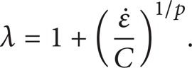
This material model is described by the expression (1) [19], based on the Cowper-Symonds model [19 –21], which scales the yield stress by a strain rate dependent factor:

σ_{y} = [1 + {(\frac{\dot{ε}}{C})}^{1 / p}] (σ_{0} + β E_{p} ε_{eff}^{p}),

(1)

where σ₀ is initial yield stress, σ_y is yield stress, $\dot{ε}$ is strain rate, and β is varying this parameter; isotropic (β = 1) or kinematic (β = 0) hardening can be obtained. In this work, isotropic hardening is supposed, so β = 1. E_p is plastic hardening modulus, defined by (2), where E_t is the tangent modulus and E is the elastic modulus:

E_{p} = \frac{E_{t} E}{E - E_{t}},

(2)

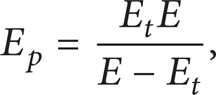
ε_eff^p is effective plastic strain, and C and p are strain rate parameters.

The following parameters have to be specified by the user in order to define properly this material when using LS-DYNA. Those parameters are as follows:

density;

Young's module;

poisson ratio;

initial yield stress;

tangent modulus;

hardening and strain rate parameters β, C, and p.

3.2. Strain Rate Dependent Isotropic Plasticity Model

In this model [19, 22], a load curve is used to describe the initial yield stress σ₀ as a function of effective strain rate ${\dot{ε}}_{eff}$ , and the yield stress σ_y is a function of the initial yield stress, the effective plastic strain ε_eff^p, and the plastic hardening modulus E_p obtained through (2). The yield stress for this material model is defined as

σ_{y} = σ_{0} {\dot{ε}}_{eff} + E_{p} ε_{eff}^{p},

(3)

where ${\dot{ε}}_{eff}$ is the effective strain rate.

In this case, material density and Poisson ratio are defined as scalar parameters, but the other properties can be defined as a function of effective strain rate. So, the entries for the model are as follows:

density;

poisson ratio;

load curve for defining the Young's module versus effective strain rate;

load curve for defining the initial yield stress versus effective strain rate;

load curve for defining the tangent modulus versus effective strain rate;

load curve for defining the Von Mises stress at failure versus effective strain rate.

3.3. Piecewise Linear Isotropic Plasticity Model

This is a multilinear elastic-plastic material option that allows stress versus strain curve input and strain rate dependency [19, 21, 23, 24]. Yield stress is expressed as

σ_{y} = λ [σ_{0} + f_{h} (ε_{eff}^{p})],

(4)

where the hardening function f_h(ε_eff^p) can be specified in tabular form. Otherwise, linear hardening is assumed as

f_{h} (ε_{eff}^{p}) = E_{p} ε_{eff}^{p} .

(5)

The parameter λ accounts for strain rate effects. There are three options to obtain it. For each of these options, the user has to specify different parameters, although there are some values that are always needed:

density;

young's module;

poisson ratio;

effective plastic true strain at failure;

initial yield stress and tangent modulus (or alternatively tabular form for f_h(ε_eff^p)).

The three options can be explained as follows.

Strain rate may be accounted for using the Cowper-Symonds model, which scales the yield stress with the factor expressed in (6). In this case, the user has to specify strain rate parameters C and p:

λ = 1 + {(\frac{\dot{ε}}{C})}^{1 / p} .

(6)

A load curve which defines λ versus strain rate can be directly introduced.

Different stress versus strain curves can be provided for various strain rates. Intermediate values are found by interpolating between curves.

4. Example: Stamping Pattern Test

The pattern test selected for the deep stamping process is being used as an example of the procedure.

This test is the first of the five stages needed to manufacture the part shown in Figure 1, which belongs to the fix system of the spare tire of a Mercedes Vito. Figures 2 and 3 show different views of the real dies used in this test.

Figure 1:

Part manufactured by five stamping stages.

Figure 2:

Pattern test for the deep stamping process. Top view.

Figure 3:

Pattern test for the deep stamping process. Bottom view.

A diagram of the position of the parts at the beginning of the test can be seen in Figure 4.

Figure 4:

Pattern test for the deep stamping process.

The blank is leaned on the bed die and the process starts with the movement of the blankholder, which applies a load to hold the blank once contact is established between them. After that, punch begins to go down, deforming the blank to obtain the part shown in Figure 5.

Figure 5:

Deformed blank obtained by pattern test.

Deformed blank was measured with a Mitutoyo coordinate measuring machine (Figure 6), and the dimension used to be compared with simulation results is shown in Figure 7.

Figure 6:

Mitutoyo coordinate measuring machine.

Figure 7:

Dimension used to compare experimental and simulation results.

5. Finite Element Simulation

As is used to do in simulation of stamping processes [5, 8, 11, 25, 26], it is divided into two major steps:

an explicit analysis that includes the blank and the dies to determine the sheet metal deformation during the stamping process;

an implicit analysis to predict the sheet metal springback deformations after the removal of the dies.

It is also common in sheet metal forming analysis to include only the surface of the dies in the finite elements model and define them as rigid entities [5]. This allows using shell elements for meshing the dies. Due to the aspect ratio of the blank, it has also been meshed with shells elements (Figure 8).

Figure 8:

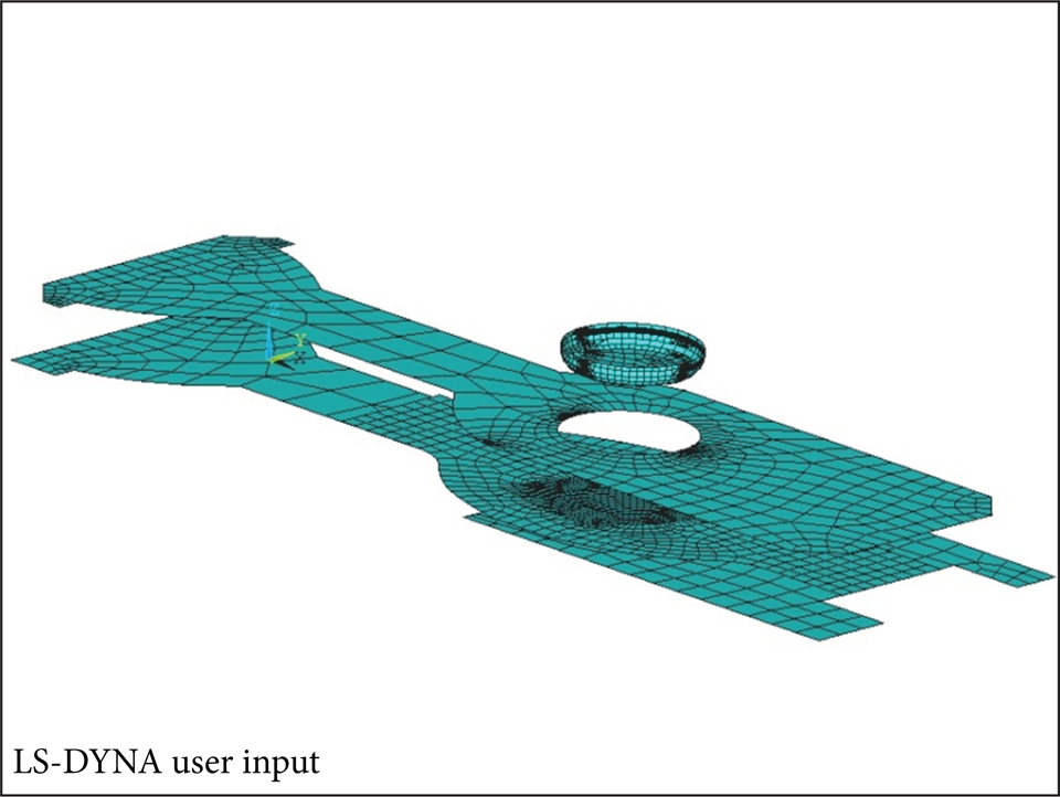
Finite element model of the dies and the blank.

Regarding the question of the material model, a nonlinear isotropic hardening model has been implemented. These isotropic hardening plasticity models that include the initial material anisotropy are the industry standards for the sheet metal process simulation and are assumed to be accurate enough [26].

Contacts between the blank and the dies have been defined using an automatic surface-to-surface contact algorithm and defining appropriate friction coefficients.

Finally, boundary and loading conditions have been specified by fixing degrees of freedom of the dies or by applying displacements and loads to them to simulate the real process (Table 1).

Table 1:

Loads and displacements used in the pattern test simulation.

TIME (s)	Punch displacement (mm)	Blankholder displacement (mm)	Blankholder load (N)

0	0	0	0
0.5	−38	−25	−90000
1	−78.5	−49.998	−90000
1.5	−116.498	−49.998	−90000
2	−78.5	−49.998	−90000
2.5	−38	−25	−90000
3	0	0	0

Deformed blank, after springback simulation, can be seen in Figure 9.

Figure 9:

Deformed blank after springback simulation.

6. Developed Application

As can be seen in previous section, building the finite element model is a hard duty, specially using high-level software as LS-DYNA.

Usually, these commercial applications are not easy to use, and the designer must employ a lot of time and effort in learning how to use them.

Because of that, an application to automate the finite element simulation has been designed [17]. This application is programmed in Matlab and offers the user a very friendly windows environment.

Since pattern tests are fixed and well known, there is no need to introduce any new parameter or command in the simulation model, just those related to material parameters. Taking this into account, the process has been programmed and it can run “blindly” for the user; that is to say that there is no need for his intervention during the simulation; furthermore, the user does not need to know how it works.

All the information that has to be introduced to define parts geometry, contact properties, loads, movements, and meshing is already collected in a subroutine that can be read by the finite element software.

Exposed procedure can be seen in Figure 10, where stages that require user intervention are drawn with solid line and those that can run “blindly” are drawn with broken line. It can be summed up as follows.

By means of the windows environment, the user chooses the kind of pattern test that is being simulated and introduces initial values for the material parameters. As a result, a text file is generated and the finite element software begins to run.

Initially, the user has to specify four different values for the material parameters, so the program will do four simulations over the same model, in order to have enough data to do an optimization.

ANSYS-LS-DYNA reads this text file, as well as the geometry of the parts (created with any CAD program) and the subroutine that includes the command orders to execute the simulations.

The value obtained for the dimension shown in Figure 7 in each simulation is stored in a text file that can be read by the MATLAB application in order to do the optimization process.

Figure 10:

Exposed procedure diagram.

7. Optimization Procedure

Once the simulation results are obtained they have to be compared with experimental ones, obtained from the physical pattern test.

This stage is also automated and only needs the user intervention in order to set the tolerance limit.

The procedure is the following.

Values obtained in the first four simulations are compared with the experimental measure.

If any of these comparisons fall inside tolerance limits, material parameters used in that simulation are considered valid.

If no one of the simulation results is accurate enough, a linear interpolation is performed to obtain new material parameters that will be used in a new simulation.

The procedure described in 1-2-3 is repeated until one of the simulation results is accurate enough. In each step, the new simulation result obtained is added to the interpolation data, as well as the material parameters used in that simulation. By doing so, in each step the interpolation process is a little bit more accurate than in previous steps, because it is built with more information.

Finally, the user gets the material parameters that allow to obtain a simulation result that falls inside tolerance limits. All the procedures that have been performed to obtain them have run hiddenly to the user, as can be seen in Figure 10.

8. Materials Models Study

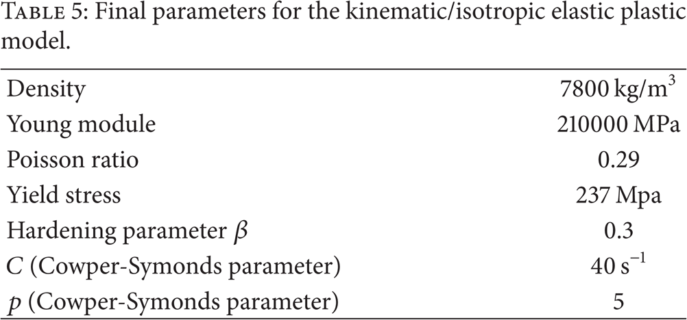
8.1. Kinematic/Isotropic Elastic Plastic Model

In this case, basic parameters like density, Poisson ratio, and Young's module will remain constant, as long as they are not expected to vary too much from one steel to another. They adopt the following values (see Table 2).

Table 2:

Initial parameters for the kinematic/isotropic elastic plastic model.

Density	7800 kg/m³
Young module	210000 MPa
Poisson ratio	0.29

So, the study is focused on the influence of those parameters that define the plastic and dynamic behavior of the material.

8.1.1. Hardening Parameter β

This parameter has a major influence in stamping processes with several steps, in which the material plasticizes more than once. Since this is not the case, it is expected that the influence of β is minimal. In spite of it, simulations have been carried out to validate this supposition, with β values of 0, 0.3 [27], and 1. As it was expected, obtained results were identical.

In following simulations, β = 0.3 is assumed.

Even in process with several stages, it can be also pointed that, looking at (1), the hardening parameter has minor influence if the tangent modulus is quite small relative to the initial yield stress (this occurs when the material has low strain hardening). This is the case of this example, so, even if the blank plasticizes again, the influence of β will not be very important.

8.1.2. Strain Rate Parameters in the Cowper-Symonds Model C and p

In this case, initial values have been selected according to examples provided by LS-DYNA users guide [28]. Starting with p = 5 and C = 40 s⁻¹, different values of C and p have been tested in order to study their influence in final results. Table 3 collects these values and the obtained depth.

Table 3:

Influence of C and p parameters.

Parameter C (s⁻¹)	Parameter p	Depth (mm)

10	5	15.8407
40	5	15.8805
100	5	15.9192
40	3	15.8974
40	7	15.8325

According to these values, it can be concluded that multiplying C by 10, produces a variation of less than 0.5% in the result. Analogous, multiplying p by 2.33 produces a variation of 0.4% in the result. Since variations in the final depth are not very important, initial values of p = 5 and C = 40 s⁻¹ have been kept.

8.1.3. Tangent Modulus

After several simulations with different values for the tangent modulus, it has been observed that values over 25000 MPa produce wrinkles in the blank. It was also seen that values over 3000 MPa produce stress values that are over the material limits. Because of that, a tangent modulus of 2000 MPa has been adopted.

8.1.4. Yield Stress

Without a doubt, this is the most important parameter in the characterization of this material model. Table 4 shows the results obtained by simulating the process with different values of the Young module.

Table 4:

Influence of the Young module.

Young module (MPa)	Depth (mm)

220	15.92
230	15.8982
237	15.8805
245	15.8383
250	15.8246

As can be seen, not very large variations (about 13.6%) produce significant differences in the final depth (about 0.6%). It can also be observed that for σ₀ = 237 MPa the final depth is 15.8805 mm, very close to the depth obtained from the real test (15.88 mm).

Table 5 shows the combination of parameters that lean to best results for this material model.

Table 5:

Final parameters for the kinematic/isotropic elastic plastic model.

Density	7800 kg/m³
Young module	210000 MPa
Poisson ratio	0.29
Yield stress	237 Mpa
Hardening parameter β	0.3
C (Cowper-Symonds parameter)	40 s⁻¹
p (Cowper-Symonds parameter)	5

8.2. Strain Rate Dependent Isotropic Plasticity Model

Initially, density, Young module, and poisson ratio kept the values used in the previous material model (see Table 2). However, Young module can be defined by a curve that represents it versus the strain rate. This possibility has been also studied as shown below.

8.2.1. Yield Stress

Yield stress has been defined by the load curve shown in Figure 11, which relates yield stress to effective strain rate.

Figure 11:

Load curve for defining the initial yield stress versus effective strain rate.

Three load curves have been implemented: an original one, obtained from the material by a real traction test, and two modified curves (shown in broken line) used to analyze the influence of this parameter. Results are shown in Table 6.

Table 6:

Influence of the yield stress in the strain rate dependent model.

Multiplier factor	Depth (mm)

0.8	15.7871
0.9	15.6797
1	15.7132

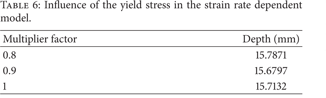
In this case, varying the yield stress about 25%, results vary about 0.5%.

8.2.2. Tangent Modulus

As has been explained previously, the use of the strain rate dependent isotropic plasticity model allows to introduce the tangent modulus as function of the strain rate. By defining this load curve, a final depth of 15.8474 mm has been obtained. This represents a variation of a 0.85% regarding the initial value of 15.7132 mm.

8.2.3. Young's Module

Other possibility of this material model is to introduce a load curve to define the Young's module as a function of the strain rate. There are references [20] that have established that the variation is not very important for strain rates higher than 2000 s⁻¹. In this case, a final depth of 15.7132 mm has been obtained. This result, as well as bibliographical fonts, concludes that Young's module can be considered as constant in this material model, since results do not change significantly by considering its dependency to strain rate.

8.3. Piecewise Linear Isotropic Plasticity Model

This material model can be defined in three different ways. All of them have been analyzed, and for all of them initial values of density, Young module, and Poisson ratio are the same as those shown in Table 2. Another needed value is the tangent modulus. A value of 2000 MPa has been used in order to keep the same values used with other models.

8.3.1. Strain Rate Is Accounted for Using the Cowper-Symonds Model

Cowper-Symonds parameters C and p have to be introduced in order to use (6). Initial yield stress and tangent modulus (or alternatively tabular form for f_h(ε_eff^p)) are also needed. In this case, C and p have the same values as in the original model (C = 40 s⁻¹ and p = 5), and f_h(ε_eff^p) has been introduced as a curve shown in Figure 12, which corresponds to a constant tangent modulus of 2000 MPa and a constant initial yield stress of 237 MPa.

Figure 12:

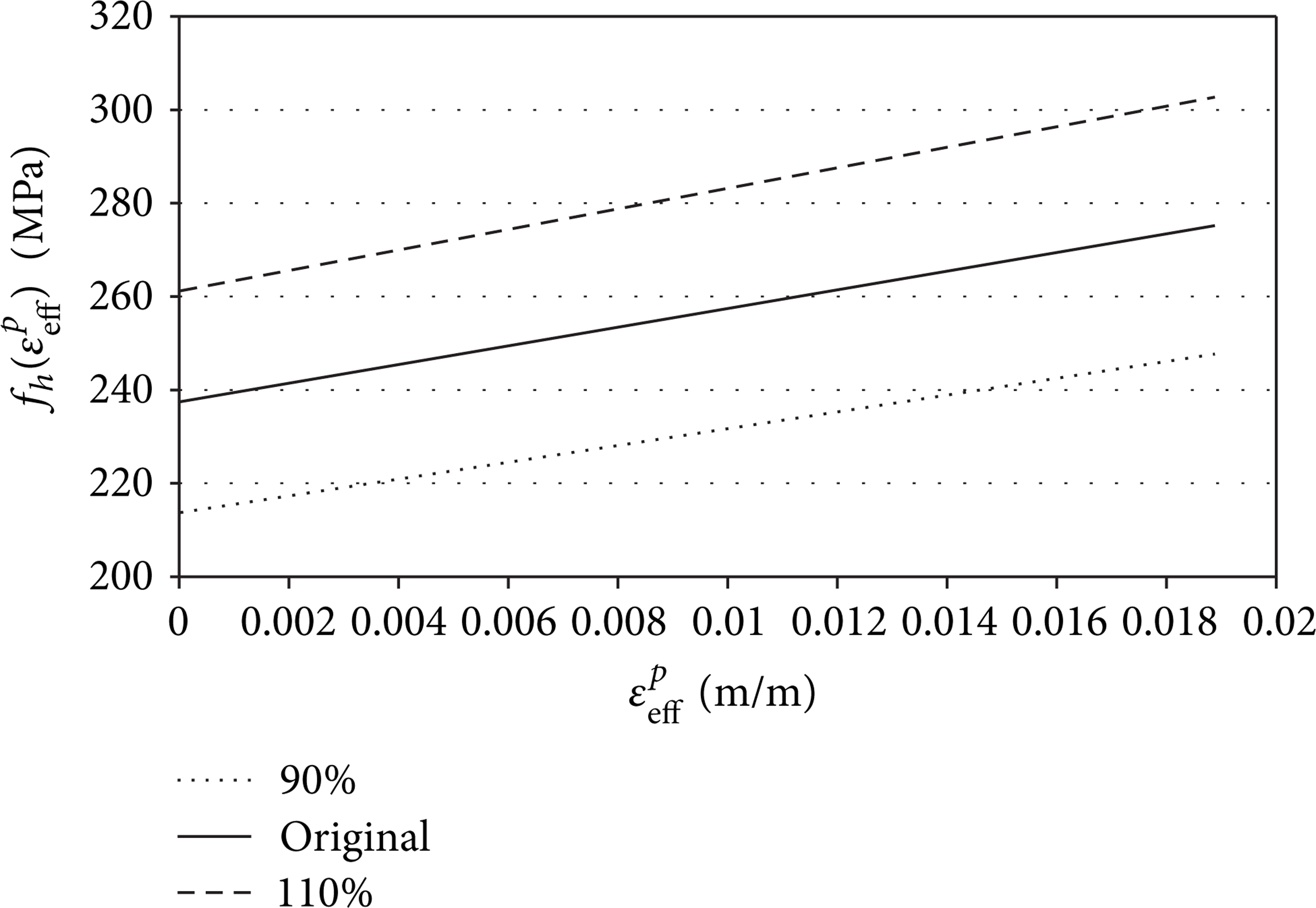
Curve to introduce f_h(ε_eff^p) in the piecewise linear isotropic plasticity model.

This curve has been modified by multiplier factors obtaining other two curves also plotted in Figure 12. Table 7 shows the results of the three simulations, which vary about 0.4% by varying f_h(ε_eff^p) about 22%. Multiplier factors have been also applied to the effective plastic strain (for a given strain, the stress is less than before, so the elastic recovering is smaller). For this assumption, by varying ε_eff^p about 11%, results vary about 0.27% (see Table 8).

Table 7:

Obtained depths for different multiplier factors applied to f_h(ε_eff^p).

Multiplier factor	Depth (mm)

0.9	15.9108
1	15.8888
1.1	15.8484

Table 8:

Obtained depths for different multiplier factors applied to the effective plastic strain.

Multiplier factor	Depth (mm)

0.95	15.9088
1	15.8888
1.05	15.8653

8.3.2. Load Curve Which Defines λ versus Strain Rate Is Directly Introduced

Instead of applying the Cowper-Symonds model, parameter λ involved in (6) can be directly introduced by a curve like the one shown in Figure 13. In this case, a final depth of 15.9838 mm has been obtained, which represents a 0.6% difference with respect to the constant λ case.

Figure 13:

Curve to define the scale parameter λ versus strain rate.

8.3.3. Different Stress versus Strain Curves Is Provided for Various Strain Rates

Ten different curves have been introduced in order to define the stress-strain relation. Strain rates have been selected according to the real ones, and they vary from 0.0004 s⁻¹ to 8 s⁻¹. Obtained depth is 15.8791 mm, just a 0.005% away from the real measured depth.

9. Obtained Results

Pattern test exposed previously has been examined as an example of the proposed optimization process.

Firstly, a deep analysis has been done to adjust all the parameters that can influence the simulation result and that do not depend on the material, that is, mesh size and boundary conditions. These parameters have been adjusted taken into account previous knowledge and real results obtained over well-known materials.

Once that the model is accurate enough for these known situations it is time for adjusting the parameters of a high-strength steel.

In the experimental test, the displacement of the punch is 16.5 mm. For this value, the final depth of the manufactured part, measured by the MMC machine, is 15.9 mm.

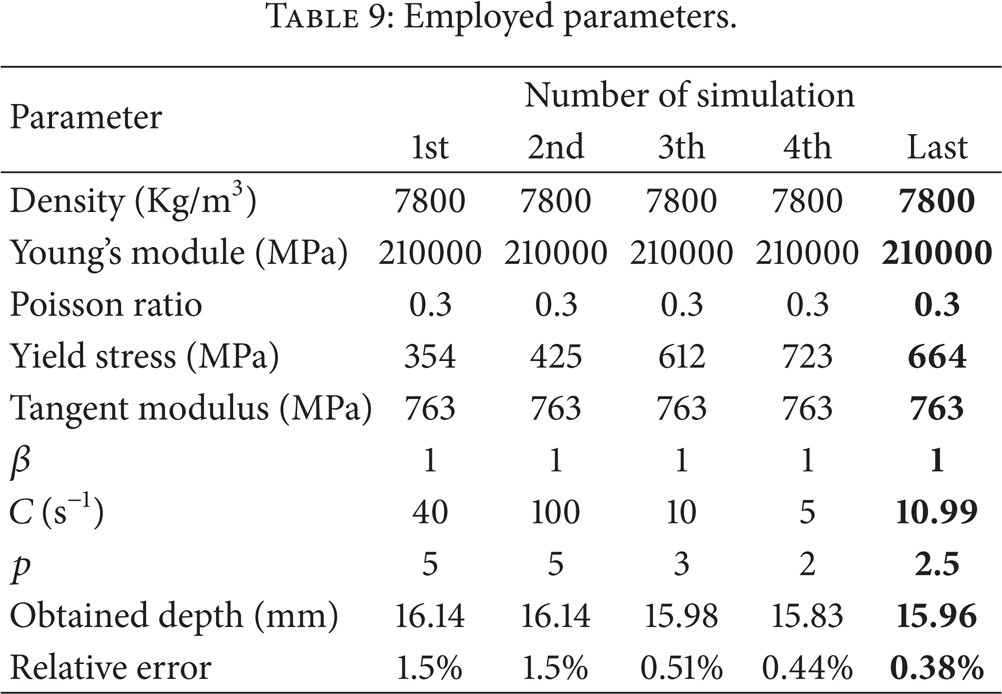
Initial values for the material parameters and the depths obtained for each combination can be seen in Table 9. The last column shows the parameters values obtained after optimization, considering a tolerance limit for the relative error of 0.5%.

Table 9:

Employed parameters.

Parameter	Number of simulation
Parameter	1st	2nd	3th	4th	Last

Density (Kg/m³)	7800	7800	7800	7800	7800
Young's module (MPa)	210000	210000	210000	210000	210000
Poisson ratio	0.3	0.3	0.3	0.3	0.3
Yield stress (MPa)	354	425	612	723	664
Tangent modulus (MPa)	763	763	763	763	763
β	1	1	1	1	1
C (s⁻¹)	40	100	10	5	10.99
p	5	5	3	2	2.5
Obtained depth (mm)	16.14	16.14	15.98	15.83	15.96
Relative error	1.5%	1.5%	0.51%	0.44%	0.38%

To validate these results, obtained parameters have been used in a new deep stamping process. Dies employed in it are shown in Figure 14 and deformed blank can be seen in Figure 15.

Figure 14:

Second simulation dies.

Figure 15:

Second simulation deformed blank.

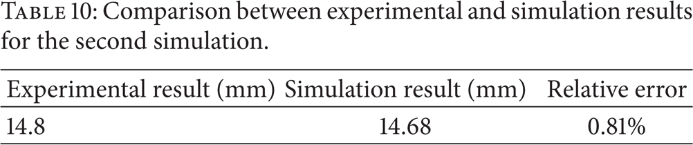
In this case, the dimension used to validate the model is the one shown in Figure 16. A comparison between results obtained through simulation and by means of the real test is shown in Table 10.

Table 10:

Comparison between experimental and simulation results for the second simulation.

Experimental result (mm)	Simulation result (mm)	Relative error

14.8	14.68	0.81%

Figure 16:

Dimension used to compared experimental and simulation results in the second simulation.

10. Conclusions

According to previous expositions and results, the following can be concluded.

A procedure to simulate real sheet metal forming processes by means of finite elements has been established.

Such a procedure has been automated and allows performing simulations with no user intervention, avoiding the difficulty of using a high-level program as LS-DYNA.

By using this automated procedure, a methodology to adjust material parameters has been developed.

Experimental tests used to validate simulation results are real applications of the industry instead of benchmark theoretical tests. This allows using previous knowledge of the designer to particularize material characterization for each kind of process and avoids building specific tooling.

Parameters involved in each material model have been identified and their influence in final results has been quantified. This is very useful to fit material properties in other simulations.

In the characterization of the three tested models, the most important parameter is the yield stress.

In the strain rate dependent isotropic plasticity model and in the piecewise linear isotropic plasticity model, considering the variation of the Young's module with the strain rate does not modify results significantly, so quite accurate results can be obtained by using a constant value. This option requires less knowledge of the material.

The kinematic/isotropic elastic plastic model is the simplest one and the more appropriate when the material behavior is not well known.

The piecewise linear isotropic plasticity model can be the more accurate, but many material parameters have to be obtained by experimental tests on real specimens.

Parameters obtained by this methodology lead to very accurate simulation results and can be used in other simulations that involve the same kind of test and the same material.

Conflict of Interests

The authors declare that there is no conflict of interests regarding the publication of this paper.

References

Buranathiti

and Kositpipat

, “Analysis and design of body jack case stamping for fewer production steps,” Journal of Materials Processing Technology, vol. 205, no. 1–3, pp. 451–458, 2008.

Oudjene

Penazzi

, and Batoz

J.-L.

, “Towards the three-dimensional FE analysis of rapid prototyping tools for sheet metal stamping process,” Finite Elements in Analysis and Design, vol. 43, no. 8, pp. 611–619, 2007.

Samuel

, “Numerical and experimental investigations of forming limit diagrams in metal sheets,” Journal of Materials Processing Technology, vol. 153–154, no. 1–3, pp. 424–431, 2004.

Silva

M. B.

Baptista

R. M. S. O.

, and Martins

P. A. F.

, “Stamping of automotive components: a numerical and experimental investigation,” Journal of Materials Processing Technology, vol. 155–156, no. 1–3, pp. 1489–1496, 2004.

Tekkaya

A. E.

, “State-of-the-art of simulation of sheet metal forming,” Journal of Materials Processing Technology, vol. 103, no. 1, pp. 14–22, 2000.

Wei

and Yuying

, “Multi-objective optimization of sheet metal forming process using Pareto-based genetic algorithm,” Journal of Materials Processing Technology, no. 1–3, pp. 499–506, 2008.

Song

J.-H.

Huh

, and Kim

S.-H.

, “A simulation-based design parameter study in the stamping process of an automotive member,” Journal of Materials Processing Technology, vol. 189, no. 1–3, pp. 450–458, 2007.

Narasimhan

and Lovell

, “Predicting springback in sheet metal forming: an explicit to implicit sequential solution procedure,” Finite elements in analysis and design, vol. 33, no. 1, pp. 29–42, 1999.

Taylor

Cao

Karafillis

A. P.

, and Boyce

M. C.

, “Numerical simulations of sheet-metal forming,” Journal of Materials Processing Tech, vol. 50, no. 1–4, pp. 168–179, 1995.

10.

Gau

J. T.

, A Study of the Influence of the Bauschinger Effect on Springback in Two-Dimensional Sheet Metal Forming. Center For Advanced Materials and Manufacturing of Automotive Components, The Ohio State University, 1999.

11.

Firat

, “U-channel forming analysis with an emphasis on springback deformation,” Materials and Design, vol. 28, no. 1, pp. 147–154, 2007.

12.

Ling

Y. E.

Lee

H. P.

, and Cheok

B. T.

, “Finite element analysis of springback in L-bending of sheet metal,” Journal of Materials Processing Technology, vol. 168, no. 2, pp. 296–302, 2005.

13.

Chen

M. H.

Gao

Zuo

D. W.

, and Wang

, “Application of the forming limit stress diagram to forming limit prediction for the multi-step forming of auto panels,” Journal of Materials Processing Technology, vol. 187–188, pp. 173–177, 2007.

14.

Morestin

Boivin

, and Silva

, “Elasto plastic formulation using a kinematic hardening model for springback analysis in sheet metal forming,” Journal of Materials Processing Technology, vol. 56, no. 1–4, pp. 619–630, 1996.

15.

Buranathiti

and Numisheet

C. J.

, “Benchmark2005 analysis on forming of an automotive underbody cross member: benchmark 2,” in Proceedings of the 6th International Conference and Workshop on Numerical Simulation of 3D Sheet Metal Forming Process (NUMISHEET '05), Smith

Zhang

Wang

C. T.

, Eds., p. 1113, AIP Conference Proceedings, Detroit, Mich, USA, 2005.

16.

Buranathiti

and Cao

, “Numisheet2005 benchmark analysis on forming of an automotive deck lid inner panel: benchmark 1,” in Proceedings of the 6th International Conference and Workshop on Numerical Simulation of 3D Sheet Metal Forming Processes (NUMISHEET '05), pp. 996–1003, usa, August 2005.

17.

Gauchía

Álvarez-Caldas

Quesada

, and Román

J. L. San

, “Material parameters in a simulation of metal sheet stamping,” Proceedings of the Institution of Mechanical Engineers D, vol. 223, no. 6, pp. 783–791, 2009.

18.

Lstc, “Ls-Dyna: User's Manual,” Tech. Rep. Version 971, LSTC, Livermore, Calif, USA, 2006.

19.

Hallquist

J. O.

, “Ls-Dyna Theoretical Manual,” Tech. Rep., LSTC, Livermore, Calif, USA, 1998.

20.

Cowper

G. R.

and Symonds

P. S.

, “Strain Hardening and Strain Rate Effects in the Impact Loading of Cantilever Beams,” Tech. Rep. 28, Brown University, Providence, RI, USA, 1958.

21.

Dietenberger

Buyuk

, and Kan

C. D.

, Development of A High StrAin-RAte Dependent Vehicle Model, Bamberg, Germany, 2005.

22.

Lihua

Xuefan

Qiang

, “Characterization of dynamic behavior of Pb-free material 95.7Sn3.8Ag0.5Cu and its determination of dynamic constitutive model parameters,” in Proceedings of the International Conference on Thermal, Mechanical and Multi-Physics Simulation and Experiments in Microelectronics and Micro-Systems (EuroSimE '08), April 2008.

23.

Peixinho

and Pinho

A. C. M.

, “Dent resistance of aluminium and magnesium alloys,” Proceedings of the Institution of Mechanical Engineers D, vol. 220, no. 9, pp. 1191–1198, 2006.

24.

Zhu

, “Modeling-technique for reliability assessment of portable electronic product subjected to drop impact loads,” in Proceedings of the 53rd Electronic Components and Technology Conference, pp. 100–104, May 2003.

25.

Esat

Darendeliler

, and Gokler

M. I.

, “Finite element analysis of springback in bending of aluminium sheets,” Materials and Design, vol. 23, no. 2, pp. 223–229, 2002.

26.

Micari

Forcellese

Fratini

Gabrielli

, and Alberti

, “Springback evaluation in fully 3-D sheet metal forming processes,” CIRP Annals, vol. 46, no. 1, pp. 167–137, 1997.

27.

García

C. M.

Celentano

D. J.

, and Flores

F. G.

, Simulación Numérica Y Validación Experimental Del Proceso De Embutición Profunda: Aplicación A Un CAso Industrial, Mecánica Computacional, 2003.

28.

Ansys , “Ansys Ls-Dyna User's Guide. Ansys Release 10.0,” Tech. Rep., ANSYS, Canonsburg, Pa, USA, 2005.

Material Characterization for FEM Simulation of Sheet Metal Stamping Processes

Abstract

1. Introduction

2. Experimental Experience: Pattern Test

3. Material Models Selection

3.1. Kinematic/Isotropic Elastic Plastic Model

3.2. Strain Rate Dependent Isotropic Plasticity Model

3.3. Piecewise Linear Isotropic Plasticity Model

4. Example: Stamping Pattern Test

5. Finite Element Simulation

6. Developed Application

7. Optimization Procedure

8. Materials Models Study

8.1. Kinematic/Isotropic Elastic Plastic Model

8.1.1. Hardening Parameter β

8.1.2. Strain Rate Parameters in the Cowper-Symonds Model C and p

8.1.3. Tangent Modulus

8.1.4. Yield Stress

8.2. Strain Rate Dependent Isotropic Plasticity Model

8.2.1. Yield Stress

8.2.2. Tangent Modulus

8.2.3. Young's Module

8.3. Piecewise Linear Isotropic Plasticity Model

8.3.1. Strain Rate Is Accounted for Using the Cowper-Symonds Model

8.3.2. Load Curve Which Defines λ versus Strain Rate Is Directly Introduced

8.3.3. Different Stress versus Strain Curves Is Provided for Various Strain Rates

9. Obtained Results

10. Conclusions

Conflict of Interests

References