Maximizing Lifetime of Three-Dimensional Corona-Based Wireless Sensor Networks

Abstract

In a wireless sensor network (WSN), the energy of nodes closer to the sink node is usually exhausted sooner than others. This is known as the energy hole problem, which heavily affects the lifetime of the network. In this work, we study the lifetime maximization problem of a three-dimensional corona-based WSN with uniformly distributed sensor nodes and data transmission workload. We first derive the optimal configuration of the first layer of the corona to maximize the lifetime of the network. Then, we propose two strategies to configure nodes outside the first layer: the equal energy strategy (EES) which minimizes the number of hops to transmit data from sensor nodes to the sink and the local optimal energy (LOE) which stands for the fact that under this strategy each individual layer reaches its minimal energy consumption. Furthermore, the optimal equal distance strategy (OEDS) which is a simple deployment strategy was proposed to prolong the lifetime of the network by optimizing layer number k.

1. Introduction

Wireless sensor network (WSN) consists of a large number of autonomous sensors to monitor physical conditions of an area-of-interest. Sensor nodes typically use batteries as the power supply, and replacing the batteries may be very inconvenient in practise. Therefore, energy efficiency is one of the most crucial problems in the design and implementation of WSN [1]. Tremendous research work has been done to reduce the energy consumption of WSN to extend their lifetime (see Section 2 for a brief review of related work).

In many WSN systems, sensor nodes send the collected data to the sink nodes by multihop transmission [2, 3]. In such systems, the energy of sensor nodes closer to the sink node is exhausted faster than others because of traffic imbalance among sensor nodes. This is known as the energy hole problem. Xu et al. [4] reported that when the energy of sensor nodes that are one hop away from the sink node is completely exhausted, nodes farther away still have up to 93% of their initial energy. Therefore, it is a big challenge to balance the sensor node energy depletion and increase the lifetime of large-scale WSN systems.

In this paper, we study the lifetime maximization problem of a larger-scale three-dimensional WSN with uniform sensor node distribution. Comparing with one- and two-dimensional WSN, three-dimensional WSN has received little attention in literatures. However, three-dimensional WSN is useful in many environmental monitoring applications. Examples include the GreenOrbs project [5], Wagyromag, and sea monitoring [6]. A three-dimensional monitoring system would help people to get more intuitive and accurate sensor data. The WSN in this study is based on the corona structure, where the whole three-dimensional monitoring area is a globe, and the globe is divided into layers by concentric spheres. The nodes in the same layer are configured with the same transmission distance (which decides the transmission energy consumption of the node). A sensor node sends data to some nodes in the layer one step closer to the sink node, and finally the nodes in the most inner layer send data to the sink node [7, 8]. The problem is how to divide whole monitoring area into layers and correspondingly configure the sensor node transmission distances to maximize the lifetime of the WSN.

Since all the sensing data from the whole monitoring area are delivered to the sink node via sensor nodes in the most inner layer (also called the first layer), the energy consumption of the first layer is usually the bottleneck of the whole network. We first study how to design the first layer to maximize the WSN lifetime. We observe that it may lead to low energy efficiency if the first layer is either too large or too small and quantitatively derive the optimal width of the first layer to maximize the WSN lifetime.

Based on the above optimal design of the first layer, we propose two strategies to design other layers. The equal energy strategy (EES) layers the monitoring area in the way that each layer has the same energy consumption speed. EES has the property of minimizing the total number of layers and thus minimizes the number of hops to transmit data from each sensor node to the sink node (given a fixed width of the first layer that maximizes the network lifetime as discussed above), which is beneficial to improve the communication reliability. However, on the other hand, EES may lead to a greater total energy consumption of the whole network. Then a local optimal energy (LOE) strategy has been proposed to achieve an optimal energy depletion of each individual layer. At last, we propose equal distance strategy (OEDS), which layers the monitoring area in the way that each layer has the same width. This simple strategy has a lower total energy consumption than EES and less layer number than LOE.

The remaining part of the paper is organized as follows: Section 2 provides a brief review of related work. Section 3 defines the problem model, including the energy consumption model and the sensor node deployment model. Section 4 presents the optimal width configuration of the first layer to maximize the network lifetime. Sections 5 and 6 present the two strategies EES and LOE to layer the area outside the first layer. Section 7 presents OEDS to layer the whole network with an optimized number of layers. Section 8 evaluates the proposed methods by experiments. Section 9 presents system parameters setting rules and sensor deployment guidelines, and imbalance energy consumption in EDS has also been discussed.

2. Related Work

Shah and Rabaey [9] considered the energy-aware routing problem for low energy ad hoc sensor networks. They observed that frequent usage of the lowest energy paths may not be optimal for the network lifetime and long-term connectivity, which used suboptimal paths occasionally to provide substantial gains in system lifetime. The energy consumption is more balanced when the traffic is sent through different routes. They used probabilistic forwarding to send traffic through different routes. However, it added considerable design complexity on individual sensor nodes. Simulation shows that the network lifetimes can be increased by up to 40% compared to the previous schemes such as directed diffusion routing.

Chattopadhyay et al. [10] proposed a single hop sensor deployment algorithm SHSD. This work considered an irregular terrain with obstacles with two types of sensor nodes. One type is client sensor nodes, which are homogeneous with the same sensing and communication coverage. The other type is server nodes, which are heterogeneous while communication coverage is larger than sensing coverage. Each WSN has a server and four clients. Sensor data by client nodes would be communicated to server nodes. Server node can communicate directly with its neighboring server nodes. A moving object can be tracked by a WSN and reported to its neighbor WSN without involving the client nodes, which decreases traffic workload. However, the gain in the deployment algorithm is needed to look for WSN (for 5 sensors together) instead of finding location of individual nodes for deployment.

Cheng et al. [11] studied the problem of mitigating hot spots around data sink nodes to maximize the network lifetime. They built a general model to analyze and evaluate various deployment methods, such as variable-range transmission power control with optimal traffic distribution and different distribution modes. In this model, they do not only study how to maximize the network lifetime but also considered extra costs factors with more complex distribution. They found that most sensor network deployment strategies can have their maximum lifetime using a linear model. The maximum achievable lifetime decreases when the network goes from one to two dimensions.

Xiong et al. [12] investigated the sensor deployment problem in network-structure environments. The target of their work is to achieve k-coverage of the network structure for minimizing the number of sensor nodes. They proved that the problem is in general NP-complete and proposed a polynomial-time optimal algorithm for the special case of the tree topologies. They also studied how to minimize the total communication cost of data collection with joint optimization of sink deployment and routing.

Slama et al. [13] proposed a simple and efficient approach to deploy multiple sinks within a large-scale WSN. They used graph partitioning techniques to determine a balanced partition of large-scale WSN and optimize placement of different sinks over the obtained smaller subnetworks in order to minimize energy consumption of data transmissions.

Gopi et al. [14] proposed the energy optimized path unaware layered routing protocol (E-PULRP) for dense underwater 3D sensor networks. E-PURLP used a layering structure which is a set of concentric spheres around the cluster head, and then they proposed a method to choose intermediate relay nodes from source node to cluster head to guarantee network has a minimum total energy expenditure.

Liu and Mohapatra [15] proposed a greedy deployment scheme that achieves suboptimal performance and reveals the relationship among the number of sensor nodes, the desired lifetime, and the coverage distance. Caione et al. [16] extended the system lifetime by proposing a new algorithm to minimize the number of packets to transmit.

Perillo et al. [17] revealed the upper bound network lifetime of several typical scenarios by proposing a general model to study the optimal transmission range distribution in two-dimensional sensor fields. Zhao et al. [18] proposed a sleep-scheduling called virtual backbone scheduling (VBS) for redundant sensor nodes. VBS forms multiple overlapped backbones which work alternatively to prolong the network lifetime.

3. System Model

3.1. Energy Consumption Model

The energy consumption of a sensor node consists of two parts: the computation energy consumption and the communication energy consumption. In this paper, we focus on the optimization of the communication energy consumption and assume the computation energy consumption to be fixed.

We adopt the communication energy consumption model in [19]:

$$\begin{array}{cc}& E_{Tx}\left(l,d\right)=E_{\text{elec}}\times l+{ϵ}_{\text{amp}}\times l\times d^{\alpha },\\ E_{Rx}\left(l\right)=E_{\text{elec}}\times l.\end{array}$$

(1)

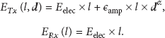
The communication energy consumption consists of the transmitting energy consumption $E_{Tx}(l,d)$ and the receiving energy consumption $E_{Rx}(l)$ . In the transmitting energy consumption $E_{Tx}(l,d)$ , l is the message size (in bits) to be transmitted, d is the distance of the transmission (in meters), $E_{\text{elec}}$ is the operational energy consumption of the transmitter to transmit each bit of message, and ${ϵ}_{\text{amp}}$ is the transmit amplifier factor. The value of l, d, $E_{\text{elec}}$ , and ${ϵ}_{\text{amp}}$ used in this paper is shown in Table 1. α is the path loss index, the value of which depends on the transmission environment. Typically, α is a constant in the range of $2\le \alpha \le 6$ [20]. The typical values of α in different transmission environment are provided in Table 2. The receiving energy consumption $E_{Rx}(l)$ only depends on the size of the message to receive.

Table 1

Radio characteristics.

d	Meters
l	Bits
$E_{\mathrm{\text{elec}}}$	50  $\mathrm{n}\mathrm{J}/\mathrm{b}\mathrm{i}\mathrm{t}$
${\mathrm{ϵ}}_{\mathrm{\text{amp}}}$	100  $\mathrm{p}\mathrm{J}/\mathrm{b}\mathrm{i}\mathrm{t}/{\mathrm{m}}^{\mathrm{\alpha }}$

Table 2

Path loss index under different environment.

Environment	α
Free space	2
Urban cellular wireless communication	2.7~3.5
Shadow fading existent in urban cellular wireless communication	3~5
Building block	4~6
Factory block	2~3

3.2. Three-Dimensional WSN Model

We have the following fundamental constraints of the sensor network model.

• (i)

There is a huge amount of sensor nodes, so it is impractical to optimize the network on the base of individual sensor nodes (e.g., set a different configuration for each individual sensor node).

(ii)

Each sensor node has a nonrenewable energy budget, while sink node has a renewable energy budget.

(iii)

The sensor nodes can adjust their transmission range by turning its transmission power level.

The WSN is deployed in the area of a globe, and the sink node is at the center of the globe. Figure 1 shows the three-dimensional WSN model. n sensor nodes are distributed around the sink node with uniform distribution in the globe (we consider the uniform distribution as an inherent property posed by the constraints of the sensor deployment procedure, the whole globe has the same density of sensor nodes). The globe is divided into k layers. Figure 1 illustrates a three-layer example, where the radius of the $i\text{th}$ layer is denoted by $r_i$ . The innermost layer is called the first layer. R is the radius of the whole globe.

Figure 1

Three-dimensional WSN Model.

The sensor nodes send sensory data to the sink node by multihop transmission. Each task in the $i\text{th}$ layer randomly chooses one node in the $(i-1)\text{th}$ layer as the destination for data delivery, and the probability of each node in the $(i-1)\text{th}$ layer to be chosen by this task is the same. The sensor nodes in the same layer all have the same transmission range configuration. Therefore, transmission range of the sensor nodes in the $i\text{th}$ layer (denoted by $d_i$ ) is the width of the corresponding layers; that is, $d_i=r_i-r_{i-1}$ . In this way, it is guaranteed that all the sensor nodes in the $i\text{th}$ layer are able to transmit data to the $(i-1)\text{th}$ layer. If we view the sink node itself as a layer with radius $r_0=0$ , the volume of each layer ${\Delta }_i$ can be obtained by subtracting the outer layer to the inner one, ${\Delta }_1=V_1-V_0=(4/3)\pi r_1^3\cdots {\Delta }_i=V_i-V_{i-1}=(4/3)\pi r_i^3-(4/3)\pi r_{i-1}^3$ , where density of sensor nodes is μ.

We make the following assumptions about our system.

• (i)

Each sensor node has the same probability to be the source of a path to sink node.

(ii)

The nodes in the same layer will not be the next hop node. Only nodes in the next layer could be the next hop.

(iii)

For $2\le i\le k$ , sensor nodes in the next layer have the same probability as the next hop node.

Note the limitation of our model; we lost the chance to send data if only the nodes in the same layer are available in the neighborhood. Some variables are defined in Table 3.

Table 3

Variables used in this paper.

Variable	Description
μ	Sensor node density for uniform distribution
∂	Data generate probability
$\partial \mathrm{\mu }$	Task density
n	Total number of sensor nodes
$n_i$	Number of sensor nodes in the ith layer
$T_{Ti}$	Transmission tasks of ith layer
$T_{Ri}$	Receiving tasks of ith layer
e	Initial battery capacity

4. Optimal Network Lifetime

Since all the sensing data from the whole monitoring area are delivered to the sink node via sensor nodes in the first layer, the energy consumption of the first layer is usually the bottleneck of the whole network. In this section, we study how to design the first layer to maximize the WSN lifetime.

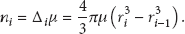
Since WSN in three-dimensional is uniform distributed, the number of sensor nodes in the $i\text{th}$ layer $n_i$ is

$$\begin{array}{cc}& n_i={\Delta }_i\mu =\frac{4}{3}\pi \mu \left(r_i^3-r_{i-1}^3\right).\end{array}$$

(2)

The sensor energy consumption mainly depends on the distance between adjacent hops and transmission workload (number of transmission tasks). The number of tasks executed by sensor node determines the transmission workload.

Since each node has equal probability as the transmission source and the destination for data delivery, the number of transmission tasks in the $i\text{th}$ layer is proportional to the total number of sensor nodes in the same layer and all the outer layers. So the number of transmission tasks of the first layer is

$$\begin{array}{cc}& T_{T1}=\frac{4}{3}\pi \partial \mu R^3.\end{array}$$

(3)

The number of receiving tasks is proportional to the total number of sensor nodes in all the outer layers, so

$$\begin{array}{cc}& T_{R1}=\frac{4}{3}\pi \partial \mu \left(R^3-r_1^3\right).\end{array}$$

(4)

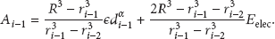
The energy consumption of each sensor node in the first layer is

$$\begin{array}{l}{E}_1\left(l,d_1\right)=\partial \frac{R^3}{r_1^3}{E}_{Tx}+\partial \frac{R^3-r_1^3}{r_1^3}{E}_{Rx}\hfill \\ =l\partial \frac{R^3}{r_1^3}ϵd_1^{\alpha }+l\partial \frac{2R^3-r_1^3}{r_1^3}{E}_{\text{elec}}.\hfill \end{array}$$

(5)

Similarly, the number of transmitting tasks and receiving tasks in $i\text{th}$ layers, $i\ge 2$ , is

$$\begin{array}{cc}& T_{Ti}=\frac{4}{3}\pi \partial \mu \left(R^3-r_{i-1}^3\right),\\ T_{Ri}=\frac{4}{3}\pi \partial \mu \left(R^3-r_i^3\right).\end{array}$$

(6)

The sensor node energy consumption in the $i\text{th}$ layer, $i\ge 2$ , is

$$\begin{array}{l}{E}_i\left(l,d_i\right)=\partial \frac{R^3-r_{i-1}^3}{r_i^3-r_{i-1}^3}{E}_{Tx}+\partial \frac{R^3-r_i^3}{r_i^3-r_{i-1}^3}{E}_{Rx}\hfill \\ =l\partial \frac{R^3-r_{i-1}^3}{r_i^3-r_{i-1}^3}ϵd_i^{\alpha }+l\partial \frac{2R^3-r_i^3-r_{i-1}^3}{r_i^3-r_{i-1}^3}{E}_{\text{elec}}.\hfill \end{array}$$

(7)

We define a and b as follows:

$$\begin{array}{cc}& a=l\partial ϵ,\\ b=l\partial E_{\text{elec}}.\end{array}$$

(8)

In the first layer, $d_1=r_1$ , by applying a, b to (7), the energy depletion in the first layer is

$$\begin{array}{l}{E}_1\left(l,d_1\right)=a{R}^3{d}_1^{\alpha -3}+b\frac{2R^3-d_1^3}{d_1^3}\hfill \\ =a{R}^3{d}_1^{\alpha -3}+2b{R}^3{d}_1^{-3}-b.\hfill \end{array}$$

(9)

As we mentioned before, $E_1$ is the bottleneck of the whole network lifetime. Therefore, our target is to minimize $E_1$ . We can get the first-order derivation of $E_1$ with respect to $d_1$ :

$$\begin{array}{cc}& E_1^{\prime }\left(l,d_1\right)=\left(\alpha -3\right)a{R}^3{d}_1^{\alpha -4}-6b{R}^3{d}_1^{-4}.\end{array}$$

(10)

For $2\le \alpha <3$ , $E_1$ is a monotone-decreasing function with respect to $d_1$ : the larger $d_1$ , the smaller $E_1$ , and we get the minimal value of $E_1^{\min }$ when $d_1$ has the maximal feasible value. In practise, there is an upper limit of the maximal transmission range of the sensor nodes, which is denoted by $t_x$ . Then, we get the minimal value of $E_1$ by

$$\begin{array}{cc}& E_1^{\min }\left(d_1\right)=a{R}^3{t}_x^{\alpha -3}+2b{R}^3{t}_x^{-3}-b.\end{array}$$

(11)

For $3\le \alpha \le 6$ , $E_1$ is fluctuated with $d_1$ and reaches its minimum value when $d_1$ satisfies $E_1^{\prime }=0$ :

$$\begin{array}{cc}& d_1={\left(\frac{6b}{a\left(\alpha -3\right)}\right)}^{1/\alpha }.\end{array}$$

(12)

By (12), we can ensure the first layer has its longest lifetime, and $E_1^{\min }$ is

$$\begin{array}{l}{E}_1^{\min }\left(l,d_1\right)=a{R}^3{\left[\frac{6b}{a\left(\alpha -3\right)}\right]}^{\left(\alpha -3\right)/\alpha }\hfill \\ +2b{R}^3{\left[\frac{6b}{a\left(\alpha -3\right)}\right]}^{-3/\alpha }-b.\hfill \end{array}$$

(13)

Summing up the above discussions, we have the following results.

Theorem 1.

In three-dimensional sensor network, all sensor nodes should be forwarded to sink node directly if their distance to the sink node is less than $\min \{{(6b/a(\alpha -3))}^{1/\alpha },t_x\}$ to have the longest network lifetime.

5. Equal-Energy Strategy

In last section, we have presented how to design the first layer to maximize the network lifetime. In the following, we study how to configure other layers based on the optimal configuration of the first layer in last section when $3<\alpha \le 6$ , and as $2\le \alpha \le 3$ is an extreme case, we can always get the maximum benefit by setting $d_i=t_x$ . There are different optimization objects in configure sensors outside the first layer. In this section, we propose a deployment strategy equal-energy strategy (EES) to reduce the number of hops it takes to transmit the sensory data to the sink. The number of hops in the transmission has a significant influence on transmission delay and system reliability. When the cluster range R is fixed, we can reduce the number of layers k by enhancing the transmission range. When $d_i=t_x$ , the network gets its minimum $k=R/t_x$ . However, under certain conditions, $d_i=t_x$ cannot guarantee the optimal network lifetime. Therefore, EES proposes a method to get the maximum transmission range of each layer based on an optimal $d_1$ . To ensure the network lifetime and avoid energy hole, set $E_1=E_2=\cdots =E_k$ , which results are each layer's transmission range, the number of layers is the smallest k value satisfying ${\sum }_{i=1}^k‍d_i\ge R$ .

To achieve this target, we must determine each $r_i$ , $2\le i\le k$ . Since $r_1$ is known from last section, this can be done iteratively, starting with $E_1(l,d_1)=E_2(l,d_2)$ :

$$\begin{array}{l}\frac{R^3}{r_1^3}ϵd_1^{\alpha }+\frac{2R^3-r_1^3}{r_1^3}{E}_{\text{elec}}=\frac{R^3-r_1^3}{r_2^3-r_1^3}ϵd_2^{\alpha }\hfill \\ +\frac{2R^3-r_2^3-r_1^3}{r_2^3-r_1^3}{E}_{\text{elec}}.\hfill \end{array}$$

(14)

Since $r_2=d_2+r_1$ , we can rewrite (14) as

$$\begin{array}{l}\frac{R^3-r_1^3}{{\left(r_1+d_2\right)}^3-r_1^3}ϵd_2^{\alpha }+\frac{2R^3-{\left(r_1+d_2\right)}^3-r_1^3}{{\left(r_1+d_2\right)}^3-r_1^3}{E}_{\text{elec}}\hfill \\ \hspace{1em}=\frac{R^3}{r_1^3}ϵd_1^{\alpha }+\frac{2R^3-r_1^3}{r_1^3}{E}_{\text{elec}}.\hfill \end{array}$$

(15)

$E_1(l,d_1)$ can be determined given the value of $r_1$ , l, ∂, μ, ${ϵ}_{\text{amp}}$ , and R. We define $A_1$ as

$$\begin{array}{cc}& A_1=\frac{R^3}{r_1^3}ϵd_1^{\alpha }+\frac{2R^3-r_1^3}{r_1^3}{E}_{\text{elec}}.\end{array}$$

(16)

Then, we have

$$\begin{array}{l}\frac{2R^3-\left(d_2^3+3d_2^2{r}_1+3d_2{r}_1^2+2r_1^3\right)}{d_2^3+3d_2^2{r}_1+3d_2{r}_1^2}{E}_{\text{elec}}\hfill \\ \hspace{1em}\hspace{1em}+\frac{R^3-r_1^3}{d_2^3+3d_2^2{r}_1+3d_2{r}_1^2}ϵd_2^{\alpha }=A_1,\hfill \end{array}$$

(17)

which can be re-written as

$$\begin{array}{l}\left(R^3-r_1^3\right)ϵd_2^{\alpha }-\left(E_{\text{elec}}+A_1\right)d_2^3-\left(3r_1{E}_{\text{elec}}+3r_1{A}_1\right)d_2^2\hfill \\ -\left(3E_{\text{elec}}{r}_1^2+3A_1{r}_1^2\right)d_2+2\left(R^3-r_1^3\right)E_{\text{elec}}=0.\hfill \end{array}$$

(18)

To calculate $r_2$ by iteration, all radii can be determined as

$$\begin{array}{l}\left(R^3-r_{i-1}^3\right)ϵd_i^{\alpha }-\left(E_{\text{elec}}+A_{i-1}\right)d_i^3\hfill \\ \hspace{1em}\hspace{1em}-\left(3r_{i-1}{E}_{\text{elec}}+3r_{i-1}{A}_{i-1}\right)d_i^2\hfill \\ \hspace{1em}\hspace{1em}-\left(3E_{\text{elec}}{r}_{i-1}^2+3A_{i-1}{r}_{i-1}^2\right)d_i\hfill \\ \hspace{1em}\hspace{1em}+2\left(R^3-r_{i-1}^3\right)E_{\text{elec}}=0.\hfill \end{array}$$

(19)

As soon as we write,

$$\begin{array}{cc}& A_{i-1}=\frac{R^3-r_{i-1}^3}{r_{i-1}^3-r_{i-2}^3}ϵd_{i-1}^{\alpha }+\frac{2R^3-r_{i-1}^3-r_{i-2}^3}{r_{i-1}^3-r_{i-2}^3}{E}_{\text{elec}}.\end{array}$$

(20)

By iteration for $2\le i\le k$ , we can obtain the radii satisfying $E_1=E_2=\cdots =E_k$ , in which assurance network has the shortest path with the longest lifetime and avoids energy hole.

6. Local Optimal Energy

The EES strategy proposed in last section can minimize the number of layers of the overall system. However, it may lead to inefficient total energy consumption since the system is configured in the way that nodes far away from the sink has the same energy consumption speed as the nodes in the innermost layer.

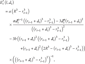
In this section, we propose another outer layer strategy local optimal energy (LOE) based on the optimal $d_1$ derived in Section 4. The object of LOE is to minimize energy consumption of each individual layer. The main idea of LOE is to get each layer's radius which makes $E_i$ reaches its minimum value.

For a certain cluster range R, we can always get the next layer's radius when we know the current layer's radius. By iterative computations, the radii of all layers can be determined and the iteration stops as soon as $r_k\ge R$ , where k is the number of layers, while still keeping an optimal each layer energy consumption. Similar with what we have done in Section 5, the iteration begins with $i=2$ , and $r_2=r_1+d_2$ :

$$\begin{array}{l}{E}_2\left(l,d_2\right)=a\frac{R^3-r_1^3}{{\left(r_1+d_2\right)}^3-r_1^3}{d}_2^{\alpha }\hfill \\ +b\frac{2R^3-{\left(r_1+d_2\right)}^3-r_1^3}{{\left(r_1+d_2\right)}^3-r_1^3}.\hfill \end{array}$$

(21)

Differentiating to $d_2$ and solving the equation $E_2^{\prime }=0$ , we can determine $d_2$ which reaches $E_2^{\min }$ :

$$\begin{array}{cc}& a\alpha \left[{\left(r_1+d_2\right)}^3-r_1^3\right]d_2^{\alpha -1}-{\left(r_1+d_2\right)}^2\left(3a{d}_2^{\alpha }+6b\right)=0.\end{array}$$

(22)

The sensor node energy consumption in the $i\text{th}$ layer is

$$\begin{array}{cc}& E_i\left(l,d_i\right)=\frac{a\left(R^3-r_{i-1}^3\right)}{{\left(r_{i-1}+d_i\right)}^3-r_{i-1}^3}{d}_i^{\alpha }+b\frac{2R^3-{\left(r_{i-1}+d_i\right)}^3-r_{i-1}^3}{{\left(r_{i-1}+d_i\right)}^3-r_{i-1}^3}.\end{array}$$

(23)

By iterative computing for $2\le i$ , differentiating to $d_i$ , we can get the first-order derivation of $E_i$ :

$$\begin{array}{l}{E}_i^{\prime }\left(l,d_i\right)\hfill \\ \hspace{1em}=a\left(R^3-r_{i-1}^3\right)\hfill \\ \hspace{1em}\hspace{1em}\times \frac{\alpha d_i^{\alpha -1}\left({\left(r_{i-1}+d_i\right)}^3-r_{i-1}^3\right)-3d_i^{\alpha }{\left(r_{i-1}+d_i\right)}^2}{{\left({\left(r_{i-1}+d_i\right)}^3-r_{i-1}^3\right)}^2}\hfill \\ \hspace{1em}\hspace{1em}-3b({\left(r_{i-1}+d_i\right)}^2\left({\left(r_{i-1}+d_i\right)}^3-r_{i-1}^3\right)\hfill \\ \phantom{\text{mmmmmii}}+{\left(r_{i-1}+d_i\right)}^2\left(2R^3-{\left(r_{i-1}+d_i\right)}^3-r_{i-1}^3\right)\phantom{\left({\left(r_{i-1}+d_i\right)}^3-r_{i-1}^3\right)})\hfill \\ \hspace{1em}\hspace{1em}\times {\left({\left({\left(r_{i-1}+d_i\right)}^3-r_{i-1}^3\right)}^2\right)}^{-1},\hfill \end{array}$$

(24)

which after some mechanical manipulations can be written as

$$\begin{array}{l}{E}_i^{\prime }\left(l,d_i\right)\hfill \\ \hspace{1em}=\left(R^3-r_{i-1}^3\right)\frac{a\alpha \left({\left(r_{i-1}+d_i\right)}^3-r_{i-1}^3\right)d_i^{\alpha -1}}{{\left((r_{i-1}+d_i{)}^3-r_{i-1}^3\right)}^2}\hfill \\ \hspace{1em}\hspace{1em}-\left(R^3-r_{i-1}^3\right)\frac{{\left(r_{i-1}+d_i\right)}^2\left(3a{d}_i^{\alpha }+6b\right)}{{\left((r_{i-1}+d_i{)}^3-r_{i-1}^3\right)}^2}.\hfill \end{array}$$

(25)

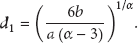
Solving the equation $E_i^{\prime }=0$ , $d_i$ can be obtained as

$$\begin{array}{cc}& a\alpha \left[{\left(r_{i-1}+d_i\right)}^3-r_{i-1}^3\right]d_i^{\alpha -1}-{\left(r_{i-1}+d_i\right)}^2\left(3a{d}_i^{\alpha }+6b\right)=0.\end{array}$$

(26)

Then, we can get total energy consumption in LOE as follows:

$$\begin{array}{cc}& {\displaystyle \sum }_{i=1}^k‍E_{\text{total}}=E_1^{\min }+E_2^{\min }+\cdots +E_i^{\min }.\end{array}$$

(27)

7. Optimal Equal-Distance Strategy

In the last two sections, we proposed two strategies EES and LOE to layer the sensor nodes outside the innermost layer. EES has the benefit of minimizing the number of layers, which is beneficial to reduce the transmission delay and enhance the transmission reliability, but has a high total energy consumption. LOE stands for the fact that under this strategy each individual layer reaches its minimal energy consumption. However, LOE often results in a considerably large number of layers, which is usually unacceptable in the design of realistic systems.

In this section, we propose the third strategy optimal equal-distance strategy (OEDS) to layer the sensor nodes outside the sink node. As suggested by its name, OEDS is a strategy based on equal-distance strategy, in which all the layers have the same width, and we prolong network lifetime by optimizing number of layers. Equal distance strategy is very simple and is widely adopted in practise. In this section, we aim to prolong network lifetime by choosing the number of layers k of the whole network (and thereby the width of each layer is $R/k$ ). We start with

$$\begin{array}{cc}& E_1\left(l,\frac{R}{k}\right)=l{k}^3\partial ϵd_1^{\alpha }+l\left(2k^3-1\right)\partial E_{\text{elec}},\end{array}$$

(28)

$$\begin{array}{cc}& E_i\left(l,\frac{R}{k}\right)=l\partial \left(\frac{k^3-{\left(i-1\right)}^3}{3i^2-3i+1}ϵd^{\alpha }+\frac{2k^3-i^3-{\left(i-1\right)}^3}{3i^2-3i+1}{E}_{\text{elec}}\right).\end{array}$$

(29)

By using substitutions a and b, we can rewrite (28) and (29) as

$$\begin{array}{cc}& E_1\left(l,\frac{R}{k}\right)=a{k}^3{d}^{\alpha }+b\left(2k^3-1\right),\end{array}$$

(30)

$$\begin{array}{cc}& E_i\left(l,\frac{R}{k}\right)=a\frac{k^3-{\left(i-1\right)}^3}{3i^2-3i+1}{\left(\frac{R}{k}\right)}^{\alpha }+b\frac{2k^3-i^3-{\left(i-1\right)}^3}{3i^2-3i+1}.\end{array}$$

(31)

The first layer's sensor energy consumption is

$$\begin{array}{cc}& E_1\left(l,\frac{R}{k}\right)=a{k}^3{\left(\frac{R}{k}\right)}^{\alpha }+b\left(2k^3-1\right).\end{array}$$

(32)

Equation (32) shows that when a, b, and R are known, $E_1$ is only determined by the number of layers k. We can adjust k to reduce the first layer's energy consumption.

For different α, we distinguish OEDS with two cases: OEDS.1 and OEDS.2. This means that sensors deployed in different environment shown in Table 2 should use different optimization strategy.

7.1. OEDS.1

When $2\le \alpha <3$ , $E_1$ is a monotonically increasing function with respect to k. $E_1$ gets the minimum value at $k_{\min }$ : the larger d, the longer network lifetime. If the sensor has a maximum transmission range $t_x$ , $k_{\min }$ can be determined as

$$\begin{array}{cc}& k_{\min }=\lceil \frac{R}{t_x}\rceil .\end{array}$$

(33)

7.2. OEDS.2

When $3\le \alpha \le 6$ , $E_1$ is fluctuated with k. The minimum value of $E_1$ can be found by computing the derivation of $E_1$ :

$$\begin{array}{cc}& E_1^{\prime }\left(l,\frac{R}{k}\right)=6b{k}^2-a{R}^{\alpha }\left(\alpha -3\right)k^{2-\alpha }.\end{array}$$

(34)

Solving the equation $E_1^{\prime }(l,R/k)=0$ , $E_1$ reaches its extremum value at

$$\begin{array}{cc}& k=\lceil {\left(\frac{a{R}^{\alpha }\left(\alpha -3\right)}{6b}\right)}^{1/\alpha }\rceil .\end{array}$$

(35)

In order to determine whether (35) is the minimum value or just an extremum value, we solve the second-order derivative of $E_1$ :

$$\begin{array}{cc}& E_1^{\mathrm{\prime \prime }}\left(l,\frac{R}{k}\right)=12bk+a{R}^{\alpha }\left(\alpha -3\right)\left(\alpha -2\right)k^{1-\alpha }>0.\end{array}$$

(36)

The second-order derivation of $E_1(l,R/k)$ is always greater than zero. So we know that $E_1(l,R/k)$ reaches its minimum value with the k value determined by (35). Then, we have the following theorem.

Theorem 2.

When we determined the number of layers k, the total energy consumption is minimum on routing along a path from the sensory data generated on the outermost layer to sink node by equal distance layering.

Proof.

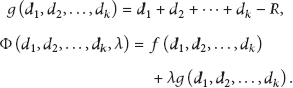
The sensor energy expenditure is divided into two categories: one is to receive data energy consumption which is only dependent on $E_{\text{elec}}$ and l and the other is to forward data energy consumption mainly dependent on $d_i$ . For the task originated at the outermost layer, no matter how we change each layer's radius, the number of receiving tasks from source node to sink node is fixed to be $(k-1)$ and the energy consumption of receiving tasks is fixed. Therefore, we can only focus on the forwarding task's energy expenditure to calculate the smallest total energy consumption from the source to the sink node. As in Figure 1, the outermost layer is the 3rd layer; that is, $k=3$ , and the number of receiving tasks along a path to the sink node is 2. It needs 3 hops to forward the sensory data to the sink node. The number of the receiving and forwarding tasks has nothing to do with each layer's radius; therefore, we only study how to set each layer's radius to minimize the total energy consumption from source to sink.

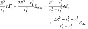
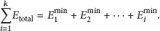
For a task generated at the outermost layer, we define ${\Phi }_k$ as the total energy consumption from source node to sink node, and ${\Phi }_k$ can be obtained as the cumulative sum of each layer's energy consumption:

$$\begin{array}{cc}& {\Phi }_k={\displaystyle \sum }_{i=1}^k‍\left(ϵ\times l\times d_i^{\alpha }+l\times E_{\text{elec}}\right).\end{array}$$

(37)

After some mathematical translation and deletion of the constant value such as $l\times E_{\text{elec}}$ , we get a new expression denoted by ${\Phi }_k^{\prime }$ :

$$\begin{array}{cc}& {\Phi }_k^{\prime }=ϵ\times l\times {\displaystyle \sum }_{i=1}^k‍d_i^{\alpha }.\end{array}$$

(38)

The problem to $\min \{{\Phi }_k\}$ can be translated into finding the minimum value of $f(d_1,d_2,\dots ,d_k)$ :

$$\begin{array}{cc}& \begin{array}{c}f\left(d_1,d_2,\dots ,d_k\right)=d_1^{\alpha }+d_2^{\alpha }+\cdots +d_k^{\alpha }\end{array}.\end{array}$$

(39)

By the method of Lagrange multipliers (Lagrange multipliers method is used to find the maxima and minima of a function subject to a set of equality constraints.), our problem of finding the minimum value of $f(d_1,d_2,\dots ,d_k)$ on condition that $d_1+d_2+\cdots +d_k=R$ can be written as

$$\begin{array}{l}g\left(d_1,d_2,\dots ,d_k\right)=d_1+d_2+\cdots +d_k-R,\hfill \\ \Phi \left(d_1,d_2,\dots ,d_k,\lambda \right)=f\left(d_1,d_2,\dots ,d_k\right)\hfill \\ +\lambda g\left(d_1,d_2,\dots ,d_k\right).\hfill \end{array}$$

(40)

λ is Lagrange's multiplier, and by partial derivative to $d_i$ and λ, we can get

$$\begin{array}{cc}& \alpha d_1^{\alpha -1}+\lambda =0\\ \alpha d_2^{\alpha -1}+\lambda =0\\ ⋮\\ \alpha d_i^{\alpha -1}+\lambda =0\\ ⋮\\ \alpha d_k^{\alpha -1}+\lambda =0\\ d_1+d_2+\cdots +d_k-R=0.\end{array}$$

(41)

The result of which

$$\begin{array}{cc}& d_1=d_2=\cdots =d_k.\end{array}$$

(42)

Accordingly we know that, when each layer has the same width, ${\Phi }_k$ can reach its minimum value, and the total energy consumption on routing along a path from the sensory data generated in the outermost layer to sink node is minimized.

8. Comparison and Analysis of Different Deployment Strategies

In this section we compare the performance among different sensor deployment strategies. The comparison considers both lifetime and the total energy consumption of the WSN.

As introduced in Section 3, the sensors are deployed around the sink node with uniform distribution in the globe, and sensor node is powered by a battery with capacity of 200 mAh, 3.3 v, and the parameter settings are as shown in Table 4.

Table 4

Parameter setting.

Network parameter	Value
l	4 bits
$\partial \mathrm{\mu }$	0.001 pkts/m3 ts
μ	$\frac{1000}{100^3}/{\mathrm{\text{m}}}^3$

8.1. Network Lifetime

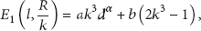
In this subsection, we compare the network lifetime and its changing trend of different strategies. Firstly, we compute the network lifetime with each strategy, respectively. In all the three strategies, the bottleneck of the network lifetime is the first layer. So the network lifetime, denoted as Γ, is computed by $\Gamma =e/E_1$ , where e is the battery capacity of each sensor node, and we assume that

$$\begin{array}{cc}& e=0.2\times 3.3\times 3600=2376\hspace{0.17em}\text{J}.\end{array}$$

(43)

(1) $2\le \alpha <3$ : in EES and LOE, $d_1$ equals the maximal transmission range when $\alpha =2$ . The first layer's energy consumption is

$$\begin{array}{cc}& E_1^{\text{EES}}\left(\mathrm{4,60}\right)=0.0083\hspace{0.17em}\text{J}.\end{array}$$

(44)

The network lifetime with EES is

$$\begin{array}{cc}& \Gamma =2376÷0.0083=286265.06.\end{array}$$

(45)

The number of layers in OEDS.1 can be computed by (33); then, we can obtain the first layer's energy consumption by

$$\begin{array}{cc}& E_1^{\text{OEDS}.1}\left(\mathrm{4,60}\right)=0.0083\hspace{0.17em}\text{J}.\end{array}$$

(46)

The network lifetime with OEDS.1 is

$$\begin{array}{cc}& \Gamma =2376÷0.0083=286265.06.\end{array}$$

(47)

Since the first layer's radii $d_1=60\hspace{0.17em}\text{m}$ in the three strategies are the same, their network lifetimes are the same, and Γ is derived as follows when $R\le t_x$ :

$$\begin{array}{cc}& \Gamma =2376÷E_1\left(4,R\right).\end{array}$$

(48)

(2) $3\le \alpha \le 6$ : without loss of generality, we set $\alpha =4$ and calculate network lifetime by the energy consumption of the first layer.

By (12), we can calculate the first layer's energy consumption in EES by

$$\begin{array}{cc}& E_1^{\text{EES}}\left(\mathrm{4,7.4008}\right)=3.9469\hspace{0.17em}\text{J}.\end{array}$$

(49)

The network lifetime in EES is

$$\begin{array}{cc}& \Gamma =2376÷3.9469=601.99.\end{array}$$

(50)

By (35), we can get layer number in OEDS.2 and compute the energy consumption of the first layer:

$$\begin{array}{cc}& E_1^{\text{OEDS}.2}\left(4,\frac{100}{14}\right)=3.9545\hspace{0.17em}\text{J}.\end{array}$$

(51)

The network lifetime in OEDS.2 is

$$\begin{array}{cc}& \Gamma =2376÷3.9545=600.83.\end{array}$$

(52)

In this case, the strategies with the optimal $d_1$ (EES and LOE) and strategy with the optimal number of layers (OEDS.2) only have a marginal difference in network lifetime. Based on the same network lifetime, the small differences in network lifetime come from the round-up to integer of k. We will compare the properties as variation of total energy consumption and the number of layers in different strategies when R changes within a reasonable range.

Figure 2(a) shows network lifetime in EDS without further optimization. The cluster range is $R=100\hspace{0.17em}\text{m}$ , and the number of layers is changed from 2 to 20; that is, the transmission range is changed from $50\hspace{0.17em}\text{m}$ to $5\hspace{0.17em}\text{m}$ . The network lifetime changes as the number of layers k increases. At the beginning, network lifetime is increasing with respect to k and reaches its peak value at $k=14$ . This is because that $d_1$ reaches its optimum value when $k=14$ , and EDS equals OEDS.2 since OEDS.2 is an optimal deployment strategy for EDS. When k continues to increase, the massive forwarding tasks result in a loss of network lifetime.

Figure 2

Network lifetime and number of layers with cluster range.

Figure 2(b) shows that, when R is changed from $100\hspace{0.17em}\text{m}$ to $180\hspace{0.17em}\text{m}$ , OEDS.2 has the same network lifetime as EES. This is because OEDS.2 optimizes the number of layers k to make $d_1$ approach its optimal value in EES. For both EES and OEDS.2, the network lifetime decreases as R increases, since the number of tasks is increasing with respect to R (increasing the number of tasks reduces the lifetime of the network). Figure 2(c) shows the number of layers in EES and OEDS.2, and we will explain this phenomenon in Section 9.

8.2. Total Energy Consumption

(1) $2\le \alpha <3$ : we assume $R=100\hspace{0.17em}\text{m}$ and $\alpha =2$ . We assume there is a maximal transmission range limit $t_x=60\hspace{0.17em}\text{m}$ .

In the following, we first introduce how to decide the radius of the first layer $d_1$ and then the radius of other layers under different deployment strategies.

EES and LOE are based on the optimal configuration of the first layer. As we stated in Section 4, when $2\le \alpha <3$ , the problem of finding the optimal $d_1$ is reduced to finding the largest transmission range. Therefore, we have $d_1=t_x=60\hspace{0.17em}\text{m}$ .

For OEDS.1, the radius of each layer equals the maximal transmission range limit in the case of $2\le \alpha <3$ as we introduced in Section 7. In particular, $d_1=t_x=60\hspace{0.17em}\text{m}$ .

Then, we decide the configuration of outer layers. The principle of EES is to extend the outer layer's transmission range satisfying $E_1=E_2=\cdots =E_k$ . Since the first layer's radius is $t_x$ , there is no room to enlarge the outer layers to grow their transmission range. To reduce the energy consumption difference between different layers, $d_2=\min \{t_x,R-d_1\}=\min \{\mathrm{60,100}-60\}=40\hspace{0.17em}\text{m}$ , and total energy consumption is

$$\begin{array}{cc}& E_{\text{total}}^{\text{EES}}={\displaystyle \sum }_{i=1}^2‍E_i=0.0092\hspace{0.17em}\text{J}.\end{array}$$

(53)

For LOE, when $\alpha =2$ and $d_1=t_x=60\hspace{0.17em}\text{m}$ , we determine each layer's radius $d_i$ by finding each layer's minimal energy consumption with (26). The results are shown in Table 5. When we set $r_2=106.2646\hspace{0.17em}\text{m}$ , total energy consumption with LOE is

$$\begin{array}{cc}& E_{\text{total}}^{\text{LOE}}={\displaystyle \sum }_{i=1}^2‍E_i=0.0091\hspace{0.17em}\text{J}.\end{array}$$

(54)

Table 5

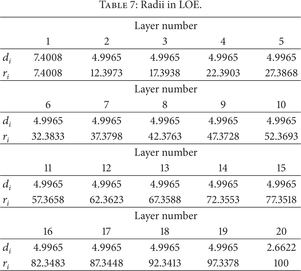
Radii in LOE.

	Layer number
	1	2
$d_i$	60	46.2646
$r_i$	60	106.2646

However, the cluster range R as the maximum value of $r_i$ is $100\hspace{0.17em}\text{m}$ , so $r_2=100\hspace{0.17em}\text{m}$ , $d_2=40$ , and total energy consumption with LOE is

$$\begin{array}{cc}& E_{\text{total}}^{\text{LOE}}={\displaystyle \sum }_{i=1}^2‍E_i=0.0092\hspace{0.17em}\text{J}.\end{array}$$

(55)

The case of OEDS.1 is similar to EES, where only two layers in this strategy, $d_1=60$ , $d_2=40$ , and total energy consumption is

$$\begin{array}{cc}& E_{\text{total}}^{\text{OEDS}.1}=E\left(\mathrm{4,60}\right)+E\left(\mathrm{4,40}\right)=0.0092\hspace{0.17em}\text{J}.\end{array}$$

(56)

Since there is almost no signal attenuation if $2\le \alpha <3$ , the energy consumption in all the three strategies is very small. When the cluster range is increased, the total energy consumption increases with R gradually for all the strategies. At the beginning, the total energy consumption of LOE is close to EES and OEDS.1. As an optimal each individual layer energy consumption strategy, total energy consumption in LOE increases slower than EES and OEDS.1. Moreover, the number of layers in LOE increases faster than the other two strategies.

$2\le \alpha <3$ is an extreme case, in which the sensor's working environment has nearly no signal attenuation. It is beneficial to reduce the number of hops by setting each layer's radius as large as possible. The comparison between different strategies is shown in Figure 3.

Figure 3

Total energy consumption.

(2) $3\le \alpha \le 6$ : we set $R=100\hspace{0.17em}\text{m}$ and $\alpha =4$ and assume the maximal transmission range limit as $t_x=60\hspace{0.17em}\text{m}$ .

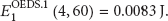
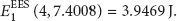
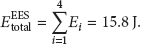
For EES, we can get the first layer's radius by (12), and the other radii $r_i$ by (19). The results are shown in Table 6. The network has 4 layers and hence total energy consumption in EES is

$$\begin{array}{cc}& E_{\text{total}}^{\text{EES}}={\displaystyle \sum }_{i=1}^4‍E_i=15.8\hspace{0.17em}\text{J}.\end{array}$$

(57)

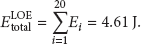
To calculate the total energy consumption in LOE, we compute each layer's radius by (26). With $R=100\hspace{0.17em}\text{m}$ , $r_i$ and $d_i$ of each layer can be calculated as in Table 7, and the total energy consumption in LOE is

$$\begin{array}{cc}& E_{\text{total}}^{\text{LOE}}={\displaystyle \sum }_{i=1}^{20}‍E_i=4.61\hspace{0.17em}\text{J}.\end{array}$$

(58)

Table 6

Radii in EES.

	Layer number
	1	2	3	4
$d_i$	7.4008	22.6453	38.2380	31.7159
$r_i$	7.4008	30.0461	68.2841	100

Table 7

Radii in LOE.

	Layer number
	1	2	3	4	5
$d_i$	7.4008	4.9965	4.9965	4.9965	4.9965
$r_i$	7.4008	12.3973	17.3938	22.3903	27.3868
	Layer number
	6	7	8	9	10
$d_i$	4.9965	4.9965	4.9965	4.9965	4.9965
$r_i$	32.3833	37.3798	42.3763	47.3728	52.3693
	Layer number
	11	12	13	14	15
$d_i$	4.9965	4.9965	4.9965	4.9965	4.9965
$r_i$	57.3658	62.3623	67.3588	72.3553	77.3518
	Layer number
	16	17	18	19	20
$d_i$	4.9965	4.9965	4.9965	4.9965	2.6622
$r_i$	82.3483	87.3448	92.3413	97.3378	100

For OEDS.2, we get $k=14$ by (35), and the energy consumption of each layer is shown in Table 8. The total energy consumption in OEDS.2 is computed by

$$\begin{array}{cc}& E_{\text{total}}^{\text{OEDS}.2}={\displaystyle \sum }_{i=1}^{14}‍E_i=5.03\hspace{0.17em}\text{J}.\end{array}$$

(59)

Table 8

Each layer's energy consumption in OEDS.2.

	Layer number
	1	2	3	4	5	6	7
$E_i$	3.954	0.564	0.207	0.105	0.063	0.041	0.028
	Layer number
	8	9	10	11	12	13	14
$E_i$	0.020	0.014	0.010	0.007	0.005	0.003	0.001

Figure 4 illustrates that, for the same α, LOE has the least energy expenditure. This suggests that our optimal method is useful to reduce the total energy consumption. However, as shown in Table 7, a huge number of layers are created in this strategy, which causes more hops of the communication than the other two methods. The total energy consumption of OEDS.2 is close to LOE with a reasonable number of hops. EES has the largest energy depletion since it reduces the number of hops by increasing the transmission range in the $i\text{th}$ layer ( $2\le i\le k$ ), and the total energy consumption of EES is k times of $E_1$ .

Figure 4

Total energy consumption.

As the cluster range R increases, the total energy consumption grows in all strategies. As shown in Figure 5(a), $E_{\text{total}}^{\text{EES}}>E_{\text{total}}^{\text{OEDS}.2}>E_{\text{total}}^{\text{LOE}}$ , the total energy consumption of EES increases faster than the other two strategies. On the other hand, the number of hops is inversely proportional to the total energy consumption as shown in Figure 5(b): $k^{\text{EES}}<k^{\text{OEDS}.2}<k^{\text{LOE}}$ . We will explain these phenomena in Section 9.

Figure 5

Total energy consumption and number of layers with cluster range.

OEDS.2 has the same lifetime as EES but less total energy consumption. However, the number of layers in OEDS.2 is more than in EES and less than LOE. Therefore, for systems that are sensitive to the number of hops in data transfer (e.g., due to the reliability reason), EES might be a good choice.

9. Discussion

In this section, we will discussion system parameter setting and propose guidelines for sensor deployment in three-dimensional corona-based wireless sensor networks. By comparing different layer's energy consumption in EDS, we will explain the phenomena of $E_{\text{total}}^{\text{EES}}>E_{\text{total}}^{\text{OEDS}.2}>E_{\text{total}}^{\text{LOE}}$ and $k^{\text{EES}}<k^{\text{OEDS}.2}<k^{\text{LOE}}$ that are left unresolved in last section.

9.1. Parameters Setting and Deployment Guidelines

The first layer's energy consumption satisfies $E^{\min }\le e$ . In Section 4, we have shown that $E_1^{\min }$ is determined by (12), so

$$\begin{array}{l}\partial R^3\{{ϵl\left[\frac{6E_{\text{elec}}}{aϵ\left(\alpha -3\right)}\right]}^{\left(\alpha -3\right)/\alpha }\hfill \\ \phantom{\text{mmm}}+2l{E}_{\text{elec}}{\left[\frac{6E_{\text{elec}}}{ϵ\left(\alpha -3\right)}\right]}^{-3/\alpha }-l{E}_{\text{elec}}\}\le e,\hfill \end{array}$$

(60)

where ϵ, l, $E_{\text{elec}}$ , and α are known. Let us denote B by

$$\begin{array}{cc}& B=ϵl{\left[\frac{6E_{\text{elec}}}{aϵ\left(\alpha -3\right)}\right]}^{\left(\alpha -3\right)/\alpha }+2l{E}_{\text{elec}}{\left[\frac{6E_{\text{elec}}}{ϵ\left(\alpha -3\right)}\right]}^{-3/\alpha }-l{E}_{\text{elec}}.\end{array}$$

(61)

We can obtain the relationship of system parameters as

$$\begin{array}{cc}& B{R}^3\partial \le e.\end{array}$$

(62)

∂ is data generation probability, and the relationship of ∂ and the number of tasks $n_T$ can be expressed as

$$\begin{array}{cc}& \partial =\frac{n}{n_T}.\end{array}$$

(63)

Then (62) can be rewritten as

$$\begin{array}{cc}& B{R}^3\frac{n}{n_T}\le e.\end{array}$$

(64)

In general, the battery capacity e is known in advance. We can set the number of tasks $n_T$ , number of sensor nodes n, and cluster range R subject to (64).

In addition, we propose two principles as the deployment guidelines to optimize the sensor network lifetime as follows.

• (i)

All sensor nodes should forward sensing data to the sink node directly if their distance to sink node is less than $\min \{t_x,(6b/a(\alpha -3){)}^{1/\alpha }\}$ .

(ii)

According to different requirements of the sensor network, we can choose different deployment strategies. EES has the least hops, LOE has the least total energy consumption, and OEDS is the easiest to implement in practise.

9.2. Imbalanced Energy Consumption in EDS

In order to check how serious the energy imbalance in EDS without optimization is, the ratio of energy consumption between the $i\text{th}$ layer and the first layer is calculated. The closer to 1 the ratio is, the more energy balance EDS is. The energy expenditure ratio between the $i\text{th}$ layer, $i\ge 2$ , and the first layer is as follows:

$$\begin{array}{l}\frac{E_i\left(l,d\right)}{E_1\left(l,d\right)}\hfill \\ =(a\frac{k^3-{\left(i-1\right)}^3}{3i^2-3i+1}{\left(\frac{R}{k}\right)}^{\alpha }\hfill \\ \phantom{\text{mm}}+b\frac{2k^3-i^3-{\left(i-1\right)}^3}{3i^2-3i+1}\phantom{{\left(\frac{R}{k}\right)}^{\alpha }})\hfill \\ \hspace{1em}\times {\left(a{k}^3{\left(\frac{R}{k}\right)}^{\alpha }+b\left(2k^3-1\right)\right)}^{-1}\hfill \\ =(\left(a{\left(\frac{R}{k}\right)}^{\alpha }+2b\right)k^3-b+b\hfill \\ \phantom{\text{mm}}-{a\left(i-1\right)}^3{\left(\frac{R}{k}\right)}^{\alpha }-b{i}^3-{b\left(i-1\right)}^3)\hfill \\ {\hspace{1em}\times \left(\left(3i^2-3i+1\right)\left(\left(a{\left(\frac{R}{k}\right)}^{\alpha }+2b\right)k^3-b\right)\right)}^{-1}\hfill \\ =\frac{1}{3i^2-3i+1}\hfill \\ \hspace{1em}\times \left(1+\frac{b-{a\left(i-1\right)}^3{R}^{\alpha }{k}^{-\alpha }-b{i}^3-{b\left(i-1\right)}^3}{a{R}^{\alpha }{k}^{3-\alpha }+2b{k}^3-b}\right).\hfill \end{array}$$

(65)

The first-order derivation of (65) with respect of k, denoted as $f(k)$ , is

$$\begin{array}{l}f(k)\hfill \\ \hspace{0.17em}=\frac{a\alpha {(i-1)}^3{R}^{\alpha }{k}^{\alpha -1}}{(3i^2-3i+1)(a{R}^{\alpha }{k}^{3-\alpha }+2b{k}^3-b)}\hfill \\ +(\left(a(3-\alpha )R^{\alpha }{k}^{2-\alpha }+6b{k}^2\right)\hfill \\ \times \left(b\left(i^3+{\left(i-1\right)}^3-1\right)+a{\left(i-1\right)}^3{R}^{\alpha }{k}^{-\alpha }\right))\hfill \\ \times {\left(\left(3i^2-3i+1\right){\left(a{R}^{\alpha }{k}^{3-\alpha }+2b{k}^3-b\right)}^2\right)}^{-1}.\hfill \end{array}$$

(66)

Obviously, when we decide sensor node transmission range, no matter how to change cluster's number of layers k, $f(k)$ is always greater than 0, which implies that $E_i(l,d)/E_1(l,d)$ is an increasing function with respect to k; namely, the unfair phenomenon of energy consumption will deteriorate with the increasing of k for all $2\le \alpha \le 6$ .

For $2\le i\le k$ , (65) describes an unbalanced phenomenon of energy consumption: the consumption of sensor nodes in the first layer is the baseline value. When $R=100\hspace{0.17em}\text{m}$ and $d=10\hspace{0.17em}\text{m}$ , the sensor energy consumption increases slower as i increases, as shown in Figure 6.

Figure 6

EDS energy consumption ratio.

In EDS, the sensor nodes deployed far from the sink node can save most of its battery energy, and the saving is more significant as i increases.

This explains the phenomenon we mentioned in last section that $E_{\text{total}}^{\text{EES}}>E_{\text{total}}^{\text{OEDS}.2}>E_{\text{total}}^{\text{LOE}}$ and $k^{\text{EES}}<k^{\text{OEDS}.2}<k^{\text{LOE}}$ when $3\le \alpha \le 6$ . For OEDS.2, the total energy consumption increases slowly as R increases. For EES, when R increases for $\Delta R$ meters, the outermost layer's transmission range and energy consumption will be higher. When the outermost layer's energy consumption is equal to the first layer's, the number of layers, $k^{\text{EES}}$ , will increase. In EES, the outer the layer is, the larger transmission range the layer has, and transmission range in OEDS.2 is close to $d_1$ in EES and hence, with the same R, EES has fewer number of layers than OEDS.2.

Assuming R increases for $\Delta R$ , the number of layers increases for n in OEDS.2 and increases for m in EES. We know that $n>m$ and $\Delta R={\sum }_{i=1}^n‍d_i={\sum }_{j=1}^m‍d_j$ , since $E_{\text{elec}}\times l$ is much smaller than ${ϵ}_{\text{amp}}\times l\times d_i^{\alpha }$ , and

$$\begin{array}{cc}& {\displaystyle \sum }_{i=1}^n‍d_i^{\alpha }<{\displaystyle \sum }_{j=1}^m‍d_j^{\alpha }.\end{array}$$

(67)

The additional energy consumption in EES must be larger than in OEDS.2. By experiments, we see that LOE is an optimal strategy in terms of total energy consumption. To reduce each layer's energy consumption, the transmission range in LOE is shorter than in OEDS.2, so $k^{\text{OEDS}.2}<k^{\text{LOE}}$ .

10. Conclusions

In this paper, we investigate the problem of sensor energy consumption in three-dimensional cluster-based WSN to optimize network lifetime. We first derive the optimal transmission range of the first layer, which is the energy bottleneck of the whole network: by optimizing $d_1$ , the network can get its maximum lifetime. When the first layer transmission range is determined, we propose two strategies to configure sensors outside the first layer with different optimization targets: EES minimizes the number of hops from sensor nodes to the sink node; LOE minimizes energy consumption of each individual layer along the path from source nodes to the sink node. Moreover, for the simplest deployment strategy OEDS, two optimal strategies had been proposed by optimizing the number of layers, which suggests a new way to prolong network lifetime besides balancing energy consumption. We also found that when the number of layers is determined, the total energy consumption is the minimum from the sensory data source to sink node by equal distance layering.

As our future work, we will implement the strategies proposed in this paper in realistic applications. Moreover, multihierarchical clustering WSN and other sensors distributions will also be studied.