Sage Journals: Discover world-class research

Abstract

The unsteady free convection boundary layer flow of a thermomicropolar fluid along a vertical plate with effect of micropolar heat conduction has been investigated. The governing equations are transformed into a new form using a method of transformed coordinates. We then use an explicit finite difference scheme to solve the transformed equations. Here, the governing equations have been reduced to the forms that are valid for entire, small, and large time regimes, by using stream-function formulation. The results obtained for the above mentioned three time regimes are compared and found to be in excellent agreement. Moreover, the effects of the physical parameters such as the viscosity parameter, K, and the heat conduction parameter, α^*, are presented in terms of the transient shear stress, couple stress, and surface heat transfer coefficient as well as transient velocity profiles, angular velocity profiles, and temperature profiles.

1. Introduction

The concept of a micropolar fluid to model fluids with microstructures which cannot be adequately is described by the classical Stokesian theory introduced by Eringen [1, 2]. According to him, examples of such fluids are animal blood, liquid crystals, and certain polymeric fluids. In such fluids the microelements possess both translational and rotational motions. The interaction of the macrovelocity field and microrotation field can be described through new material constants in addition to those for a classical Newtonian fluid.

The concept of boundary layer in micropolar fluids was first introduced by Willson [3] to study the steady, incompressible laminar flow over 2-dimensional bodies. Subsequently, the steady boundary layer flow of micropolar fluids at the stagnation point of a 2-dimensional body has been considered by Peddieson and McNitt [4]. In addition to these, Ahmadi [5] considered the steady boundary layer flow of micropolar fluids over a semi-infinite flat plate and obtained a self-similar solution. The thermal boundary layer in micropolar fluids at the stagnation point of a 2-dimensional body was considered recently by Ramachandran et al. [6] and Gorla [7]. Hossain et al. [8, 9] investigated two-dimensional mixed convection and natural convection flow of a viscous incompressible thermomicropolar fluid with uniform spin-gradient over a flat plate.

Later, Jena and Mathur [10 –12] studied the similarity solutions for the steady laminar free convection boundary layer flow of a thermomicropolar fluid past a nonisothermal vertical flat plate. Recently, a model on natural convection flow of a thermomicropolar fluid along a porous vertical surface has been studied by Hossain et al. [13]. But all the above studies pertain to steady flows.

But all the above studies pertain to steady flows. However, Gorla and Takhar [14] examined the effect of buoyancy force on an unsteady incompressible micropolar fluid in the vicinity of the lower stagnation point of a circular cylinder. More or less recent studies on transient boundary layer flow of micropolar fluid without or with buoyancy effect have been done by Kumari and Nath [15], Lok et al. [16], and Xu et al. [17]. Unsteady mixed convection flow of thermomicropolar fluid along a vertical thin cylinder and along a vertical wavy surface have been investigated in [18 –20]. Very recently, Hossain et al. [21] have studied the fluctuating free convection boundary layer flow of a thermomicropolar fluid of micropolar thermal conductivity along a vertical plate considering the small amplitude temperature oscillations about a variable surface temperature.

Here, we propose to study the unsteady free convection boundary layer flow of a thermo-micropolar fluid along a heated vertical plate with the presence of micropolar heat conduction. The reduced governing equations that are valid for entire time regimes is solved using explicit finite difference method. Asymptotic solutions for small and large time are also obtained. The results thus obtained are compared and found to be in excellent agreement. We further have examined the effect of the physical parameters, such as the vortex viscosity parameter, K, and the heat conduction parameter, α^*, in terms of the transient shear stress, couple stress, and surface heat transfer coefficients as well as transient velocity profiles, angular velocity profiles, and temperature profiles.

2. Mathematical Formalisms

A two-dimensional unsteady laminar boundary layer flow of a thermomicropolar natural convection incompressible fluid along a permeable vertical flat plate is considered. The flow configuration and the coordinate system are shown in Figure 1. The dimensionless equations of continuity, momentum, angular velocity, and energy that govern the flow are given as [10, 13, 21]

\frac{\partial u}{\partial x} + \frac{\partial v}{\partial y} = 0,

(1)

\frac{\partial u}{\partial t} + u \frac{\partial u}{\partial x} + v \frac{\partial u}{\partial y} = (1 + K) \frac{\partial^{2} u}{\partial y^{2}} + K \frac{\partial G}{\partial y} + θ,

(2)

\frac{\partial G}{\partial t} + u \frac{\partial G}{\partial x} + v \frac{\partial G}{\partial y} = (1 + \frac{K}{2}) \frac{\partial^{2} G}{\partial y^{2}} - K (2 G + \frac{\partial u}{\partial y}),

(3)

\frac{\partial θ}{\partial t} + u \frac{\partial θ}{\partial x} + v \frac{\partial θ}{\partial y} = \frac{1}{Pr} \frac{\partial^{2} θ}{\partial y^{2}} + α^{*} (\frac{\partial θ}{\partial x} \frac{\partial G}{\partial y} - \frac{\partial θ}{\partial y} \frac{\partial G}{\partial x}) .

(4)

The set of equations (1)–(4) are dimensionless which are based on the following dimensionless dependent and independent variables

\begin{matrix} x = \frac{\bar{x}}{L}, y = \frac{\bar{y}}{L}, \bar{u} = \frac{ν}{L} u, \bar{v} = \frac{ν}{L} v, \\ \bar{N} = \frac{ν}{L^{2}} G, t = \frac{ν}{L^{2}} \bar{t}, θ = \frac{g β (\bar{T} - T_{\infty}) L^{3}}{ν^{2}} . \end{matrix}

(5)

Here, $(\bar{x}, \bar{y})$ are the coordinates parallel with and perpendicular to the flat surface, respectively, $(\bar{u}, \bar{v})$ are the velocity components, t time, $\bar{N}$ the angular velocity, θ dimensionless temperature, j the microinertia per unit mass, ρ the density of the fluid, g the acceleration due to gravity, κ the thermal conductivity of the fluid, γ = (μ + κ/2)j the gyroviscosity coefficient, and α^* the micropolar heat conduction coefficient. Following Jena and Mathur [10], it is assumed that microinertia, j, is a constant and, therefore, it is set equal to a reference value, j₀ = L². Further, L is the characteristic length, $K = (κ / μ)$ is vortex viscosity parameter, μ the dynamic viscosity, Pr = (ν/α) is the Prandtl number that gives the ratio of momentum diffusivity to thermal diffusivity, ν, viscosity coefficient, α^* = (N^*/L²), is the micropolar heat conduction parameter. Corresponding boundary conditions are

\begin{matrix} u = 0, v = 0, G = - n \frac{\partial u}{\partial y}, θ = θ_{w} (x), \\ at y = 0, \\ u = 0, G = 0, θ = 0 as y ⟶ \infty . \end{matrix}

(6)

In the above equation, θ_w(x) is the prescribed surface temperature. Here, we have considered that θ_w(x) = x.

Figure 1:

Flow configuration and coordinate system.

In the meantime, Jena and Mathur [11, 12] studied the same model for steady laminar free convection flow of a thermomicropolar fluid past a nonisothermal vertical flat plate as well as for nonuniformly heated porous vertical flat plate.

The values of the physical quantities, namely, the shear stress, τ_ω, the couple-stress, m_ω, and the rate of heat transfer, q_ω, at the surface of the plate, which are important from the experimental point of view are readily obtained

\begin{matrix} τ_{ω} = (1 + K) {(\frac{\partial u}{\partial y})}_{y = 0}, m_{ω} = (1 + \frac{K}{2}) {(\frac{\partial G}{\partial y})}_{y = 0}, \\ q_{ω} = - {(\frac{\partial θ}{\partial y})}_{y = 0} . \end{matrix}

(7)

3. Methods of Solution

Here, we are investigating the present problem in three time regimes, namely, (i) entire, (ii) small, and (iii) large time regimes. The method of solutions discussed in the following section has been adopted by Hossain et al. [22] and Mahfooz et al. [23] while analyzing the problems on unsteady mixed convection boundary layer flow of viscous incompressible fluid along a symmetric wedge with variable surface temperature as well as on the radiation effects on transient magnetohydrodynamic natural convection flow with heat generation.

3.1. Solutions for Entire Time Regime (All τ)

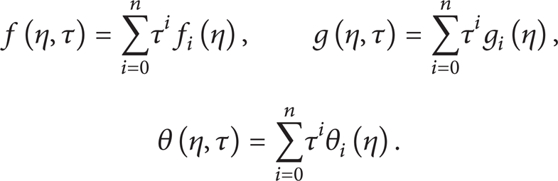
To get the solutions for entire time regime here we introduce the following group of transformations [22, 23]:

\begin{matrix} ψ = x {(1 - e^{- τ})}^{3 / 2} f (η, τ), \bar{θ} = x θ (η, τ), \\ η = y {(1 - e^{- τ})}^{- 1 / 2}, τ = x^{- 1 / 2} t . \end{matrix}

(8)

In (1), η is the similarity variable and ψ is the stream function defined by

u = \frac{\partial ψ}{\partial η}, v = - \frac{\partial ψ}{\partial x} .

(9)

That satisfies the equation of continuity (1).

Now, (1)–(4) together with the boundary conditions (6) and the transformations (8) are reduced to

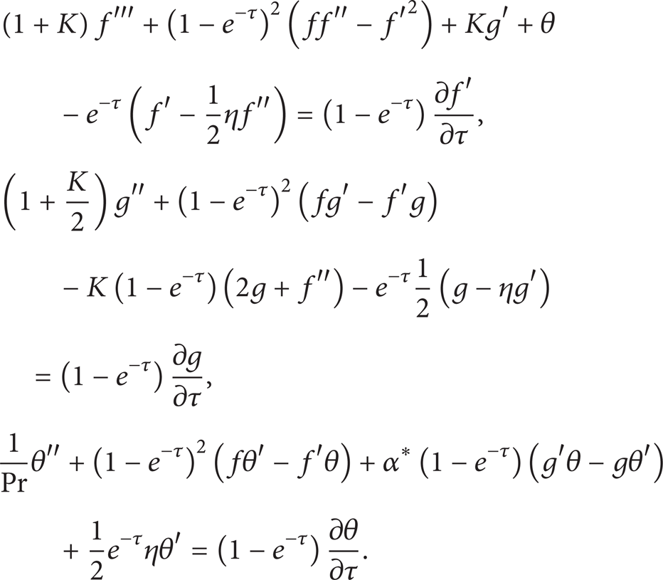
\begin{matrix} (1 + K) f^{′′′} + {(1 - e^{- τ})}^{2} (f f^{′′} - {f^{'}}^{2}) + K g^{'} + θ - e^{- τ} (f^{'} - \frac{1}{2} η f^{′′}) = (1 - e^{- τ}) \frac{\partial f^{'}}{\partial τ}, \\ (1 + \frac{K}{2}) g^{′′} + {(1 - e^{- τ})}^{2} (f g^{'} - f^{'} g) - K (1 - e^{- τ}) (2 g + f^{′′}) - e^{- τ} \frac{1}{2} (g - η g^{'}) = (1 - e^{- τ}) \frac{\partial g}{\partial τ}, \\ \frac{1}{Pr} θ^{′′} + {(1 - e^{- τ})}^{2} (f θ^{'} - f^{'} θ) + α^{*} (1 - e^{- τ}) (g^{'} θ - g θ^{'}) + \frac{1}{2} e^{- τ} η θ^{'} = (1 - e^{- τ}) \frac{\partial θ}{\partial τ} . \end{matrix}

(10)

The corresponding boundary conditions are

\begin{matrix} f (0, τ) = 0, f^{'} (0, τ) = 0, \\ g (0, τ) = - \frac{1}{2} f^{′′} (0, τ), θ (0, τ) = 1 \\ at η = 0, \\ f^{'} (\infty, τ) = 0, g (\infty, τ) = 0, θ (\infty, τ) = 0, \\ \forall 0 \leq τ \leq \infty, \end{matrix}

(11)

where primes denote the differentiation with respect to η.

The starting point to obtain the solutions of (10) is the set of the finite-difference equations obtained by spatial discretization of the transformed equations (10). The first-order central difference approximation is used for the first-order derivative with respect to η, and the second-order central difference approximation is used for the second-order derivative with respect to η. The forward differences are used for the time derivative. This discretization results in the following tridiagonal algebraic system of equations:

A_{k} Ω_{i - 1, j} + B_{k} Ω_{i, j} + C_{k} Ω_{i + 1, j} = D_{k} .

(12)

In the above equations, the subscripts k (= 1, 2, and 3) represent the functions U, θ, and φ, respectively. i (= 1, 2,…, M) and j (= 1, 2,…, N) correspond to the grid points in η and τ directions, respectively. The coefficients A_k, B_k, C_k, and D_k may be obtained easily. These block tridiagonal systems for k = 1, 2, and 3 are solved by a block matrix version of the well-known Thomas algorithm. Once the function U = f′(η) is known, the function f may be found explicitly from the following relation:

f_{i, j} = f_{i - 1, j} + Δ η U_{i, j} .

(13)

The computation is started at τ = 0.0 and then marches forward until it reaches a steady state. The convergence criteria for detecting the steady state solutions are set in such a way that the difference between the values of the function f(η, τ) obtained in two consecutive time steps is less than 10⁻⁴. The computational domain is discretized in the (τ, η) space by using the step sizes of Δτ and Δη. After some experimentation, the final mesh sizes are chosen to be Δη = 0.005 and Δτ = 0.02.

Solutions obtained are thus used to get the values of nondimensional shear stress, the couple stress, and the rate of heat transfer from (5) and are then transformed to

\begin{matrix} \frac{τ_{ω}}{x} = (1 + K) {(1 - e^{- τ})}^{1 / 2} f^{′′} (0, τ), \\ \frac{m_{ω}}{x} = (1 + \frac{K}{2}) g^{'} (0, τ), \\ \frac{q_{ω}}{x} = - {(1 - e^{- τ})}^{- 1 / 2} θ^{'} (0, τ) . \end{matrix}

(14)

Numerical values of the coefficients of shear stress, the couple stress, and the rate of heat transfer are presented in tabular form as well as graphically in the following sections.

In the next subsections, we will discuss the asymptotic solutions for small and large time τ.

3.2. Asymptotic Solutions for Small Time (τ ≪ 1) Regime

For small time regime, we consider τ ≪ 1. Consequently, the value of e^−τ ≈ 1 and 1 − e^−τ ≈ τ. Thus, (15) must now be written in the following form, which is more convenient for analysis at small times:

\begin{matrix} (1 + K) f^{′′′} + τ^{2} (f f^{′′} - {f^{'}}^{2}) + (\frac{1}{2} η f^{′′} - f^{'}) + K g^{'} + θ - τ \frac{\partial f^{'}}{\partial τ} = 0, \\ (1 + \frac{K}{2}) g^{′′} + τ^{2} (f g^{'} - f^{'} g) - τ K (f^{′′} + 2 g) + \frac{1}{2} (η g^{'} - g) - τ \frac{\partial g}{\partial τ} = 0, \\ \frac{1}{Pr} θ^{′′} + τ^{2} (f θ^{'} - f^{'} θ) + α^{*} τ (g^{'} θ - g θ^{'}) + \frac{1}{2} η θ^{'} - τ \frac{\partial θ}{\partial τ} = 0 . \end{matrix}

(15)

The boundary conditions (11) become

\begin{matrix} f (0, τ) = f^{'} (0, τ) = 0, g (0, τ) = - \frac{1}{2} f^{′′} (0, τ), \\ θ (0, τ) = 1, \\ f^{'} (\infty, τ) = g^{'} (\infty, τ) = θ^{'} (\infty, τ) = 0, \forall 0 \leq τ \leq 1 . \end{matrix}

(16)

By knowing the functions f, g, and θ and their derivatives, we can readily get the values of the shear stress, the couple stress, and the rate of heat transfer, q, from the following relations.

At small values of τ (τ ≪ 1), it can easily be verified that the solutions of (15) take the following form:

\begin{matrix} f (η, τ) = \sum_{i = 0}^{n} τ^{i} f_{i} (η), g (η, τ) = \sum_{i = 0}^{n} τ^{i} g_{i} (η), \\ θ (η, τ) = \sum_{i = 0}^{n} τ^{i} θ_{i} (η) . \end{matrix}

(17)

Now, by substituting the series expressions given in (17) into (15) and picking up the terms up to the O(τ²), we get the following sets of boundary value problems:

(1 + K) f_{0}^{′′′} + \frac{1}{2} η f_{0}^{′′} - f_{0}^{'} + K g_{0}^{'} + θ_{0} = 0,

(18)

(1 + \frac{K}{2}) g_{0}^{′′} + \frac{1}{2} (η g_{0}^{'} - g_{0}) = 0,

(19)

\frac{1}{Pr} θ_{0}^{′′} + \frac{1}{2} η θ_{0}^{'} = 0,

(20)

\begin{matrix} f_{0} (0, τ) = f_{0}^{'} (0, τ) = 0, g_{0} (0, τ) = - \frac{1}{2} f_{0}^{′′} (0, τ), \\ θ_{0} (0, τ) = 1, \\ f_{0}^{'} (\infty, τ) = g_{0} (\infty, τ) = θ_{0} (\infty, τ) = 0, \forall τ \geq 0, \end{matrix}

(21)

(1 + K) f_{1}^{′′′} + \frac{1}{2} η f_{1}^{′′} - 2 f_{1}^{'} + K g_{1}^{'} + θ_{1} = 0,

(22)

(1 + \frac{K}{2}) g_{1}^{′′} - K (2 g_{1} + f_{1}^{′′}) + \frac{1}{2} (η g_{1}^{'} - g_{1}) = 0,

(23)

\frac{1}{Pr} θ_{1}^{′′} + \frac{1}{2} η θ_{1}^{'} + α^{*} (g_{0}^{'} θ_{0} - g_{0} θ_{0}^{'}) - θ_{1} = 0,

(24)

\begin{matrix} f_{1} (0, τ) = f_{1}^{'} (0, τ) = 0, g_{1} (0, τ) = - \frac{1}{2} f_{1}^{′′} (0), \\ θ_{1} (0, τ) = 0, \\ f_{1}^{'} (\infty, τ) = g_{1} (\infty, τ) = θ_{1} (\infty, τ) = 0, \\ \forall 0 \leq τ \leq \infty, \end{matrix}

(25)

(1 + K) f_{2}^{′′′} + \frac{1}{2} η f_{2}^{′′} - 3 f_{2}^{'} + f_{0} f_{0}^{′′} - f_{0}^{' 2} + K g_{2}^{'} + θ_{2} = 0,

(26)

(1 + \frac{K}{2}) g_{2}^{′′} + \frac{1}{2} η g_{2}^{'} - \frac{5}{2} g_{2} + f_{0} g_{0}^{'} - f_{0}^{'} g_{0} - K (f_{1}^{′′} + 2 g_{1}) = 0,

(27)

\frac{1}{Pr} θ_{2}^{′′} + \frac{1}{2} η θ_{2}^{'} + f_{0} θ_{0}^{'} - f_{0}^{'} θ_{0} + α^{*} (g_{0}^{'} θ_{1} + g_{1}^{'} θ_{0} - g_{0} θ_{1}^{'} - g_{1} θ_{0}^{'}) - 2 θ_{2} = 0,

(28)

\begin{matrix} f_{2} (0, τ) = f_{2}^{'} (0, τ) = 0, g_{2} (0, τ) = - \frac{1}{2} f_{2}^{′′} (0), \\ θ_{2} (0, τ) = 0, at η = 0, \\ f_{2}^{'} (\infty, τ) = g_{2} (\infty, τ) = θ_{2} (\infty, τ) = 0, \\ \forall 0 \leq τ \leq \infty . \end{matrix}

(29)

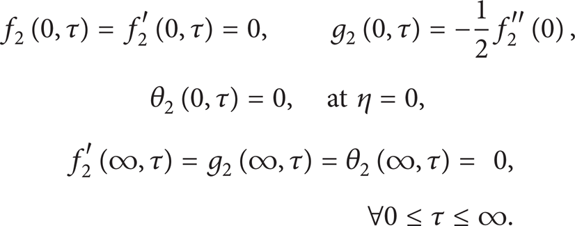
The set of equations (18)–(20), (22)–(24), and (26)–(28) are linear by nature which, although are solvable analytically, are solved numerically employing the linear shooting method (or the method of superposition). Results thus obtained for f_i″(0), g_i′(0), and θ_i′(0), i = 0, 2, are used in obtaining the values of the shear stress, the couple stress, and the rate of heat transfer, from

\begin{matrix} \frac{τ_{ω}}{x} = (1 + K) τ^{1 / 2} \sum_{i = 0}^{2} f_{i}^{′′} (0), \frac{m_{ω}}{x} = (1 + \frac{K}{2}) \sum_{i = 0}^{2} g_{i}^{'} (0), \\ \frac{q_{ω}}{x} = - τ^{- 1 / 2} \sum_{i = 0}^{2} θ_{i}^{'} (0) . \end{matrix}

(30)

For example, we have obtained the solutions of the above sets of equations for K = 1 while Pr = 9.0 and α^* = 0.25, for which we have the following expressions for shear stress, τ_ω/x, couple stress, m_ω/x, and surface heat transfer, q_ω/x:

\begin{matrix} \frac{τ_{ω}}{x} = (1 + K) τ^{1 / 2} (0.17551 + 0.00775 τ - 0.00547 τ^{2} + \dots), \\ \frac{m_{ω}}{x} = (1 + \frac{K}{2}) (0.06352 + 0.05055 τ - 0.01803 τ^{2} + \dots), \\ \frac{q_{ω}}{x} = τ^{- 1 / 2} (1.69440 + 0.04697 τ + 0.01640 τ^{2} + \dots) . \end{matrix}

(31)

Numerical values obtained from the above expressions for shear stress, couple stress, and surface heat transfer entered in Table 2 for comparison with other solutions obtained by the method discussed in forgoing section.

3.3. Asymptotic Solutions for Large Time (τ ≫ 1) Regime

Now for large time regime, (10) can be reduced to following form:

\begin{matrix} (1 + K) f^{′′′} + f f^{′′} - {f^{'}}^{2} + K g^{'} + θ - τ^{- 1} (f^{'} - \frac{1}{2} η f^{′′}) = \frac{\partial f^{'}}{\partial τ}, \\ (1 + \frac{K}{2}) g^{′′} + f g^{'} - f^{'} g - \frac{1}{2} τ^{- 1} (g - η g^{'}) - K (f^{′′} + 2 g) = \frac{\partial g}{\partial τ}, \\ \frac{1}{Pr} θ^{′′} + f θ^{'} - f^{'} θ + \frac{1}{2} τ^{- 1} η θ^{'} + α^{*} (g^{'} θ - g θ^{'}) = \frac{\partial θ}{\partial τ} . \end{matrix}

(32)

Corresponding boundary conditions are obtained as follows:

\begin{matrix} f (0, τ) = 0, f^{'} (0, τ) = 0, \\ g (0, τ) = - \frac{1}{2} f^{′′}, θ (0, τ) = 1, \\ at η = 0 . \end{matrix}

(33)

Expanding the functions involves the set of equations (32)–(33) in powers of τ⁻¹ as given below

\begin{matrix} f (η, τ) = \sum_{i = 0}^{n} τ^{- i} F_{i} (η), g (η, τ) = \sum_{i = 0}^{n} τ^{- i} G_{i} (η), \\ θ (η, τ) = \sum_{i = 0}^{n} τ^{- i} Φ_{i} (η) . \end{matrix}

(34)

Now, by using the functions given in (34) into (32)–(33) and taking the terms up to the O(τ⁻¹) we get

(1 + K) F_{0}^{′′′} + F_{0} F_{0}^{′′} - F_{0}^{' 2} + K G_{0}^{'} + Φ_{0} = 0,

(35)

(1 + \frac{K}{2}) G_{0}^{′′} + F_{0} G_{0}^{'} - F_{0}^{'} G_{0} - K (F_{0}^{′′} + 2 G_{0}) = 0,

(36)

\frac{1}{Pr} Φ_{0}^{′′} + F_{0} Φ_{0}^{'} - F_{0}^{'} Φ_{0} + α^{*} (G_{0}^{'} Φ_{0} - G_{0} Φ_{0}^{'}) = 0,

(37)

\begin{matrix} F_{0} (0, τ) = 0, F_{0}^{'} (0, τ) = 0, \\ G_{0} (0, τ) = - \frac{1}{2} F_{0}^{′′}, Φ_{0} (0, τ) = 1, \\ F_{0}^{'} (\infty, τ) = 0, G_{0} (\infty, τ) = 0, Φ_{0} (\infty, τ) = 0, \\ \forall 0 \leq τ \leq \infty, \end{matrix}

(38)

(1 + K) F_{1}^{′′′} + F_{0} F_{1}^{′′} + F_{1} F_{0}^{′′} - 2 F_{0}^{'} F_{1}^{'} + K G_{1}^{'} + Φ_{1} - (f_{0}^{'} - \frac{1}{2} η f_{0}^{′′}) = 0,

(39)

(1 + \frac{K}{2}) G_{1}^{′′} + F_{0} G_{1}^{'} + F_{1} G_{0}^{'} - (F_{0}^{'} G_{1} + F_{1}^{'} G_{0}) - K (F_{1}^{′′} + 2 G_{1}) - \frac{1}{2} (g_{0} - η g_{0}^{'}) = 0,

(40)

\begin{matrix} \frac{1}{Pr} Φ_{1}^{′′} + F_{0} Φ_{1}^{'} + F_{1} Φ_{0}^{'} - F_{0}^{'} Φ_{1} - F_{1}^{'} Φ_{0} + \frac{1}{2} η θ_{0}^{'} + α^{*} [(G_{0}^{'} Φ_{1} + G_{1}^{'} Φ_{0}) - (G_{0} Φ_{1}^{'} + G_{1} Φ_{0}^{'})] = 0, \end{matrix}

(41)

\begin{matrix} F_{1} (0, τ) = 0, F_{1}^{'} (0, τ) = 0, \\ G_{1} (0, τ) = - \frac{1}{2} F_{1}^{′′}, Φ_{1} (0, τ) = 0, \\ at η = 0, \\ F_{1}^{'} (\infty, τ) = 0, G_{1} (\infty, τ) = 0, Φ_{1} (\infty, τ) = 0, \\ \forall 0 \leq τ \leq \infty . \end{matrix}

(42)

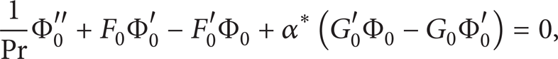
Equations (35) to (37) are the leading order equations and represent the steady state flow at large τ. The same set of equations were obtained by Hossain et al. [21] as the steady mean part of the fluctuating flow of the thermomicropolar fluid past a flat surface that was maintained at small amplitude oscillating temperature about a nonuniform steady mean temperature. We should further mention that Jena and Mathur [10] in studying the laminar free convective flow of a thermomicropolar fluid past a nonisothermal vertical flat plate obtained the same set of that given above. It should be noted that the set of equations (35) to (37) are nonlinear. Hence, solutions of these equations are obtained numerically by employing the nonlinear shooting method. Typical values of F″(0), G′(0), and Φ′(0) obtained are thus compared with that of Jena and Mathur [10] in Table 1.

Table 1:

Numerical values of the coefficients of shear stress, surface heat transfer, and couple stress for K = 0.1 and 0.25, while Pr = 9.0 and α^* = 1.0 in a comparison.

Comparison	K = 0.1			K = 0.25
Comparison	F″(0)	− G′(0)	− θ′(0)	F″(0)	− G′(0)	− θ′(0)

Jena and Mathur [10]	0.1558	0.0365	0.3675	0.1480	0.0389	0.3561
Present	0.15574	0.03652	0.36764	0.14829	0.03883	0.35787

Table 2:

Numerical values of shear stress, τ_ω/x, couple stress, m_ω/x, and surface heat transfer, q_ω/x, while K = 1.0 and α^* = 0.25 against τ.

τ	τ_ω/x		m_ω/x		q_ω/x
τ	All τ	Asymptotic	All τ	Asymptotic	All τ	Asymptotic

0.01	0.03428	0.03512^s	0.09375	0.09604^s	17.21207	16.94869^s
0.02	0.04851	0.04968^s	0.09449	0.09679^s	12.17307	11.98789^s
0.05	0.07681	0.07866^s	0.09667	0.09901^s	7.70340	7.58826^s
0.10	0.10887	0.11146^s	0.10020	0.10260^s	5.45267	5.37353^s
0.20	0.15459	0.15817^s	0.10692	0.10937^s	3.86422	3.81126^s
0.4	0.22004	0.22482^s	0.11907	0.12129^s	2.74688	2.71293^s
0.6	0.27066	0.27514^s	0.12974	0.13182^s	2.25728	2.26240^s
1.0	0.35052	0.35557^s	0.14740	0.14407^s	1.77750	1.7577^s
1.50	0.42721	0.42823^s	0.16417	0.14819^s	1.49132	1.47113^s
1.86	0.47167	0.46641^s	0.17345	0.14278^s	1.34835	1.34805^s
20.0	0.68453	0.65616^l	0.20662	0.14273^l	1.11083	1.55191^l
30.0	0.68454	0.66755^l	0.20613	0.20743^l	1.09406	1.10524^l
40.0	0.68455	0.67324^l	0.20613	0.20784^l	1.09410	1.10245^l
50.0	0.68455	0.67666^l	0.20613	0.20808^l	1.09410	1.10077^l
60.0	0.68455	0.67893^l	0.20824	0.20739^l	1.20824	1.09965^l
70.0	0.68455	0.68056^l	0.20613	0.20836^l	1.09410	1.09886^l
80.0	0.68455	0.68178^l	0.20613	0.20845^l	1.09410	1.09826^l
90.0	0.68455	0.68273^l	0.20613	0.20851^l	1.09410	1.09779^l
100.0	0.68455	0.68349^l	0.20613	0.20857^l	1.09410	1.09742^l

s stands for small time and l stands for large time.

Here, we have obtained the solutions of equations up to the O(τ⁻¹) using the nonlinear shooting method. Once we know the values of F_i″(0), G_i′(0), and Φ_i′(0) for i = 0, 1, we may obtain the numerical values of the coefficients of shear stress, couple stress, and surface heat transfer from the expressions that are given below

\begin{matrix} \frac{τ_{ω}}{x} = (1 + K) \sum_{i = 0}^{1} τ^{- i} F_{i}^{′′} (0), \frac{m_{ω}}{x} = (1 + \frac{K}{2}) \sum_{i = 0}^{1} τ^{- i} G_{i i}^{'} (0), \\ \frac{q_{ω}}{x} = - \sum_{i = 0}^{1} τ^{- i} Φ_{i}^{'} (0) . \end{matrix}

(43)

For example, taking K = 1.0, Pr = 9.0, and α^* = 0.25, we get the following expressions for shear stress, τ_ω/x, couple stress, m_ω/x, and surface heat transfer, q_ω/x:

\begin{matrix} \frac{τ_{ω}}{x} = (1 + K) (0.34516 - 0.34155 τ^{- 1} + \dots), \\ \frac{m_{ω}}{x} = (1 + \frac{K}{2}) (0.13937 - 0.03245 τ^{- 1} + \dots), \\ \frac{q_{ω}}{x} = - (- 1.09407 - 0.33523 τ^{- 1} + \dots) . \end{matrix}

(44)

Numerical values thus obtained for shear stress, τ_ω/x, couple stress, m_ω/x, and surface heat transfer, q_ω/x, are entered in Table 2 for values of τ while K = 1.0 and α^* = 0.25. This table also contained the asymptotic values of the above physical quantities for comparison. The comparison shows excellent agreement with the perturbation solutions for smaller value of τ up to 1.48 and for large value of τ from 40.0 that are obtained for all τ.

4. Results and Discussion

In the above sections, we have analyzed the problem of unsteady natural convection laminar boundary layer flow of thermomicropolar viscous incompressible fluid along a nonuniformly heated vertical surface. The governing dimensionless boundary layer equations are transformed into suitable forms appropriate for entire, small, and large time regimes. Solutions of the resulting equations are then obtained numerically and the results are depicted in terms of the transient shear stress, τ_ω/x, couple stress, m_ω/x, and surface heat transfer, q_ω/x. Here, we have discussed the effects of the physical parameters, such as the micropolar heat conduction parameter, α^*, the vortex viscosity parameter, K, and τ_ω/x, m_ω/x, and q_ω/x against the time variable τ. The present analysis of the problem has been carried out considering the fluid for which Pr = 9.0 [10]. Further results have been presented and discussed in terms of axial velocity, angular velocity, and the temperature profiles with effect of the aforementioned physical parameters.

4.1. Effect of Micropolar Heat Conduction Parameter, α^*, on Transient Shear Stress, Couple Stress Coefficients, and Surface Heat Transfer

The effects of the micropolar heat conduction parameter, α^*, on the transient shear stress, τ_ω/x, the couple stress, m_ω/x, and the surface heat transfer coefficient, q_ω/x, are presented, respectively, in Figures 2(a) to 2(c) taking value of the vortex viscosity parameter, K, equal to 1.0. It is seen from these figures that as the micropolar heat conduction, α^*, leads to decrease of the value of the shear stress as well as the heat transfer, there is increase in the couple stress. These happen due to the fact that increase in the value of micropolar thermal conductivity enhances the fluid's thermal conductivity. These figures also contain the representative values of τ_ω/x, m_ω/x, and q_ω/x obtained from the asymptotic solution for different values of α^*. One can claim that the asymptotic values in the smaller and larger time regimes agree excellently with all time solutions. This claims that the results presented here for all-time regime are accurate and hence may be useful for the experimentalists.

Figure 2:

Numerical values of (a) shear stress, (b) couple stress, and (c) surface heat transfer coefficient for different values of α^* against values of τ while Pr = 9.0 and K = 1.0.

4.2. Effect of Vortex Viscosity Parameter, K, on Transient Shear Stress, Couple Stress Coefficients, and Surface Heat Transfer

Now, we show the effect of the vortex viscosity parameter, K, on the transient shear stress, τ_ω/x, couple stress, m_ω/x, and surface heat transfer coefficient, q_ω/x. Figures 3(a)–3(c) depict the values of τ_ω/x, m_ω/x, and q_ω/x for K = 1.0, 3.0, and 5.0 while α^* = 1 against τ. From these figures, one can see that an increase in the value of the vortex-viscosity leads to increase in shear stress but decrease in the couple stress and the surface heat transfer. This is expected because increasing value of the vortex viscosity will increase the total viscosity of the fluid.

Figure 3:

Numerical values of (a) shear stress, (b) couple stress, and (c) surface heat transfer coefficient for different values of K against values of τ while α^* = 1.0.

4.3. Transient Axial Velocity, Angular Velocity, and Temperature Profiles for Different Time (τ)

The transient axial velocity, angular velocity, and temperature profiles are shown in Figures 4(a)–4(c) against η for values of τ in [0, 8] while vortex-viscosity parameter K = 1 and micropolar thermal conductivity parameter α^* = 5.0. It is seen from Figures 4(a) and 4(c) that the axial velocity and the temperature profiles increase with the increase of time which leads to increase in both the momentum boundary thicknesses. On the other hand, one can also see that in the vicinity of the surface, that is, in the region η ≤ 2 (approximately), the angular velocity profile decreases, whereas these profiles increase with the increase of time in the region η > 2. Further, we notice that all the profiles reach to the asymptotic profile or the steady state profile at larger value to time parameter τ. In this case, we found the maximum value of τ to be 8 to reach the profiles at steady state.

Figure 4:

Numerical values of (a) velocity profiles, (b) angular velocity profiles, and (c) temperature profiles for different values of τ against η when Pr = 9.0 and K = 1.0.

4.4. Effect of Micropolar Heat Conduction Parameter, α^*, on Axial and Angular Velocity and Temperature Profiles

Here, we show the effect of micropolar thermal conductivity, α^*, on the transient axial velocity, angular velocity, and the temperature profiles at τ = 2.0 while K = 1.0 through Figures 5(a) to 5(c), respectively. In this case α^* = 0.0, 0.5, 1.0, 1.5, and 2.0. It is clear from these figures that the axial velocity, angular velocity, and temperature profiles increase due to increase in micropolar thermal conductivity, α^*. But, owning to increase in the heat conduction parameter, no significant effect on the angular velocity profile is observed.

Figure 5:

(a) Axial velocity profiles, (b) angular velocity profiles, and (c) temperature profiles for different values of α^* against η at τ = 2 when Pr = 9.0 and K = 1.0.

4.5. Effect of Vortex Viscosity Parameter, K, on Axial Velocity, Angular Velocity, and Temperature Profiles

The effect of increasing values of the vortex viscosity parameter, K, on the transient axial velocity, angular velocity, and temperature profiles are depicted in Figures 6(a)–6(c) at τ = 2.0 and α^* = 0.25. From Figure 6(a), it can be seen that, within the region η < 1.8, the velocity profile increases due to increase in the value of the vortex-viscosity of the fluid, whereas, this leads to decrease in the velocity profile in the region η > 1.8. This implies that increase in the vortex viscosity leads to decrease in the momentum boundary layer thickness. We further observe that the angular velocity profile decreases owing to increase in the value of K which leads to reduction in the angular momentum boundary layer thickness. Finally, one can see that there is no significant contribution to the temperature profile due to increase in the vortex viscosity parameter K.

Figure 6:

Numerical values of (a) velocity profiles, (b) angular velocity profiles, and (c) temperature profiles for different values of K against η at τ = 2 when Pr = 9.0 and α^* = 0.25.

5. Conclusions

In this paper, we have investigated an unsteady free convection boundary layer flow of a thermomicropolar fluid along a heated vertical plate, considering the presence of micropolar heat conduction. The reduced governing equations that are valid for entire time regimes are solved using explicit finite difference method. Asymptotic solutions for small and large time are also obtained. The results obtained are thus compared and found to be in excellent agreement. From the present investigation, we may conclude the following.

The micropolar heat conduction, α^*, leads to decrease in the shear stress as well as the heat transfer, whereas this leads to increase in the couple stress.

There are decrease in the value of shear stress and the couple stress and increase in the surface heat transfer owing to increase in the value of the vortex viscosity.

Both the axial velocity and angular velocity along with temperature profile increase due to increase in the micropolar thermal conductivity, α^*.

Increase in the vortex viscosity leads to decrease in the momentum boundary layer thickness but leads to reduction of the angular momentum boundary layer thickness.

Footnotes

Nomenclature

Conflict of Interests

The authors declare that there is no conflict of interests regarding the publication of this paper.

Acknowledgment

The authors would like to thank the respected reviewers for their valuable suggestions for improving the quality of the paper.

References

Eringen

A. C.

, “Theory of micropolar fluids,” Journal of Applied Mathematics and Mechanics, vol. 16, pp. 1–18, 1966.

Eringen

A. C.

, “Theory of thermomicropolar fluids,” Journal of Mathematical Analysis and Applications, vol. 38, pp. 480–496, 1972.

Willson

A. J.

, “Boundary-layer in micropolar liquids,” Proceedings of the Cambridge Philosophical Society, vol. 67, no. 2, pp. 469–476, 1970.

Peddieson

and McNitt

R. P.

, “Boundary layer theory for a micropolar fluid,” Recent Advances in Engineering Science, vol. 5, pp. 405–476, 1970.

Ahmadi

, “Self-similar solution of imcompressible micropolar boundary layer flow over a semi-infinite plate,” International Journal of Engineering Science, vol. 14, no. 7, pp. 639–646, 1976.

Ramachandran

Chen

T. S.

, and Armaly

B. F.

, “Mixed convection in stagnation flows adjacent to vertical surfaces,” Journal of Heat Transfer, vol. 110, no. 2, pp. 373–377, 1988.

Gorla

R. S. R.

, “Micropolar boundary layer flow at a stagnation point on a moving wall,” International Journal of Engineering Science, vol. 21, no. 1, pp. 25–34, 1983.

Hossain

M. A.

and Chowdhury

M. K.

, “Mixed convection flow of micropolar fluid over an isothermal plate with variable spin gradient viscosity,” Acta Mechanica, vol. 131, no. 3–4, pp. 139–151, 1998.

Hossain

M. A.

Chowdhury

M. K.

, and Gorla

R. S. R.

, “Free convection flow of thermomicropolar fluid along a vertical plate with nonuniform surface temperature and surface heat flux,” International Journal of Numerical Methods for Heat and Fluid Flow, vol. 9, no. 5, pp. 568–585, 1999.

10.

Jena

S. K.

and Mathur

M. N.

, “Similarity solutions for laminar free convection flow of a thermomicropolar fluid past a non-isothermal vertical flat plate,” International Journal of Engineering Science, vol. 19, no. 11, pp. 1431–1439, 1981.

11.

Jena

S. K.

and Mathur

M. N.

, “Free convection in the laminar boundary layer flow of a thermomicropolar fluid past a vertical flat plate with suction/injection,” Acta Mechanica, vol. 42, no. 3–4, pp. 227–238, 1982.

12.

Jena

S. K.

and Mathur

M. N.

, “Mixed convection flow of a micropolar fluid from an isothermal vertical plate,” Computers and Mathematics with Applications, vol. 10, no. 3, pp. 291–304, 1984.

13.

Hossain

M. Mosharof

Roy

N. C.

, and Hossain

M. A.

, “Boundary layer fow and heat transfer in a micropolar fuid past a permeable flat plate,” Theoretical and Applied Mechanics Letters, vol. 40, pp. 403–425, 2012.

14.

Gorla

R. S. R.

and Takhar

H. S.

, “Unsteady mixed convection boundary layer flow of a micropolar fluid near the lower stagnation point on a cylinder,” International Journal of Engineering Fluid Mechanics, vol. 4, pp. 337–351, 1991.

15.

Kumari

and Nath

, “Unsteady incompressible boundary layer flow of a micropolar fluid at a stagnation point,” International Journal of Engineering Science, vol. 22, no. 6, pp. 755–768, 1984.

16.

Lok

Y. Y.

Amin

, and Pop

, “Unsteady boundary layer flow of a micropolar fluid near the rear stagnation point of a plane surface,” International Journal of Thermal Sciences, vol. 42, no. 11, pp. 995–1001, 2003.

17.

Liao

S. J.

, and Pop

, “Series solutions of unsteady boundary layer flow of a micropolar fluid near the forward stagnation point of a plane surface,” Acta Mechanica, vol. 184, no. 1–4, pp. 87–101, 2006.

18.

Kumari

and Nath

, “Unsteady mixed convection flow of a thermomicropolar fluid on a long thin vertical cylinder,” International Journal of Engineering Science, vol. 27, no. 12, pp. 1507–1518, 1989.

19.

Wang

C. C.

and Chen

C. K.

, “Transient force and free convection along a vertical wavy surface in micropolar fluids,” International Journal of Heat and Mass Transfer, vol. 44, no. 17, pp. 3241–3251, 2001.

20.

Rani

H. P.

and Kim

C. N.

, “A transient natural convection of micropolar fluids over a vertical cylinder,” Heat and Mass Transfer/Waerme- und Stoffuebertragung, vol. 46, no. 11–12, pp. 1277–1285, 2010.

21.

Hossain

M. Mosharof

Roy

N. C.

Mandal

A. C.

, and Hossain

M. A.

, “Fluctuating flow of thermomicropolar fluid past a vertical surface,” Applications and Applied Mathematics, vol. 8, pp. 128–150, 2013.

22.

Hossain

M. A.

Bhowmick

, and Gorla

R. S. R.

, “Unsteady mixed-convection boundary layer flow along a symmetric wedge with variable surface temperature,” International Journal of Engineering Science, vol. 44, no. 10, pp. 607–620, 2006.

23.

Mahfooz

S. M.

Hossain

M. A.

, and Gorla

R. S. R.

, “Radiation effects on transient magnetohydrodynamic natural convection flow with heat generation,” International Journal of Thermal Sciences, vol. 58, pp. 79–91, 2012.

Transient Natural Convection Flow of Thermomicropolar Fluid of Micropolar Thermal Conductivity along a Nonuniformly Heated Vertical Surface

Abstract

1. Introduction

2. Mathematical Formalisms

3. Methods of Solution

3.1. Solutions for Entire Time Regime (All τ)

3.2. Asymptotic Solutions for Small Time (τ ≪ 1) Regime

3.3. Asymptotic Solutions for Large Time (τ ≫ 1) Regime

4. Results and Discussion

4.1. Effect of Micropolar Heat Conduction Parameter, α*, on Transient Shear Stress, Couple Stress Coefficients, and Surface Heat Transfer

4.2. Effect of Vortex Viscosity Parameter, K, on Transient Shear Stress, Couple Stress Coefficients, and Surface Heat Transfer

4.3. Transient Axial Velocity, Angular Velocity, and Temperature Profiles for Different Time (τ)

4.4. Effect of Micropolar Heat Conduction Parameter, α*, on Axial and Angular Velocity and Temperature Profiles

4.5. Effect of Vortex Viscosity Parameter, K, on Axial Velocity, Angular Velocity, and Temperature Profiles

5. Conclusions

Footnotes

Nomenclature

Conflict of Interests

Acknowledgment

References

4.1. Effect of Micropolar Heat Conduction Parameter, α^*, on Transient Shear Stress, Couple Stress Coefficients, and Surface Heat Transfer

4.4. Effect of Micropolar Heat Conduction Parameter, α^*, on Axial and Angular Velocity and Temperature Profiles