
Abstract
To explore the relation between drivers' eye movements and vehicle steering performance, 25 participants were employed to drive a test vehicle on appointed tortuous routes. The drivers' visual behavior was measured while they were driving, and experiment data collected on motorway on-ramps and interchanges were used to analyze the drivers' visual characteristics. The distribution density of the fixation points showed that the drivers paid attention to the inner road edge when turning left and the outer road edge when turning right. Meanwhile, the heights of the gaze targets hardly changed. Therefore, a further investigation discovered that the gaze trajectory was parallel to the vehicle's driving trajectory on one-way curves. Then, six types of gaze trajectories were derived, and models for each type were established. Combining these models with the fact that gaze points are always distributed along the nearby road edge, it was deduced that the starting point of the gaze trajectory when driving on curves has a salient influence on the driver's gaze trajectory.
1. Introduction
Horizontal curves have long been recognized as road sections on which traffic accidents are likely to happen. Statistical analysis had shown that the accident rate and severity are highest on moderate curves, at 55% and 58%, respectively [1]. Much attention is therefore paid in the literature to investigating factors that influence accident occurrence and the characteristics of driving behavior.
Compared with the other senses, vision plays a leading role for drivers in obtaining road, traffic, and environmental information [2–4]. Gaze, saccade, and smooth tracking are the most common forms of eye movements, and it had been estimated that more than 80% of visual scanning time is accounted for by gaze and smooth tracking [5, 6]. When driving on a curved section of road, the driver operates the vehicle by steering by the right amount at the right time, depending on the information obtained visually [7–9]. Hence, the curves driving conditions had been studied in many prior pieces of research that had tried to investigate the crucial visual cues for steering and the relationship between gaze targets and vehicle driving performance. These studies had shown that, on curves, eye movements and the vehicle's steering operations are closely linked. Since the driver's gaze behavior is closely bound to the task conditions, both in spatial and temporal terms, a perfect theory or model that can be used in any situation is difficult to derive [2, 10, 11].
To date, several models had been put forward for showing how drivers extract information about road alignment and curvature and judge the appropriate amount of steering for the bend when driving around curves. The tangent-point model is the most representative one [12–16]. In this model, drivers spent much of their time looking at the tangent point on the upcoming bend. The tangent point is the moving point on the inside road edge at which the driver's gaze ray is tangential to the road edge. The tangent point is also a highly visible point and easily observable by the driver. The angular location of this point relative to the vehicle's true heading predicts the curvature of the bend: larger angles indicate greater curvatures. Thus, potentially, this angle can provide the signal needed to control steering. According to the steering angle feedback, the tangent-point model can be divided into the tangent-point targeting model and the tangent-point orientation model. In the former, drivers fixate on the tangent point and use the visual angle of the tangent point relative to the locomotor axis to judge the curvature of the bend. This model makes no specific prediction about the driver's steering. In the latter model, drivers fixate on the tangent point and actively steer so as to keep the visual angle of the tangent point in a constant horizontal direction.
Some researchers had found that the driver's gaze target is not the tangent point exactly, but a point near this particular geometric position [17–23]. Researchers holding this opinion had argued that drivers fixate on a target point along their future path, that is, a point they wish to pass through, which is near the tangent point but not necessarily equal to the tangent point. The driver observes the visual angle between the vehicle's true heading and the target point, estimates the vehicle's speed and the distance to the point, and adjusts the steering and speed.
Experimental results also had shown that the far zone beyond the tangent point is an important gaze target area during steady-state cornering [24]. This model is in line with the future-path steering model, but is difficult to reconcile with any pure tangent-point steering model. Researches advocating this model had concluded that the tangent-point steering models do not provide a general explanation of eye movements and steering during a curve-driving sequence and cannot be considered uncritically as the default interpretation when the distribution of gaze point is observed to gather in the region of the curve apex.
Based on the above statement, it was quite apparent that none of the existing steering models is suitable for all phenomena. There was no consensus on whether the actual gaze target is the tangent point itself—or some other road point in its vicinity—or on what the functional significance of the distribution of fixation point in curve driving might be.
To investigate the relationship between the driver's gaze targets and driving performance, research similar to that described above was carried out. An experiment was executed in three representative cities, and urban inhabitants were employed as subjects to drive a test vehicle on appointed tortuous routes. To eliminate the influence of traffic flow on driving and drivers' visual behavior, motorway on-ramps and interchanges were selected as the curved sections. In total, experimental data on 25 participants were collected and used in statistical analysis. From the distribution density analysis of the fixation points, it was found that drivers paid their attention on the inner road edge when turning left and the outer road edge when turning right. Besides, the heights of the gaze targets hardly change. A further investigation discovered that the gaze trajectory is parallel to the vehicle's driving trajectory on one-way curves. Finally, six types of gaze trajectory were derived and models for each type established.
2. Analysis of Gaze Trajectory Characteristics When Driving on Curves
2.1. Method and Materials
A driver's visual behavior is time dependent and space dependent. The time-varying circumstances in the driving period have a great impact on the driver's visual characteristics and gaze targets. Therefore, drivers' visual parameters should be measured together with their driving performance and the road, traffic, and environmental conditions during specific driving tasks.
The FaceLAB device was used to collect drivers' visual parameters, which were installed just in front of the driver. Visual parameters were measured using a car-fixed coordinate system, and the system was established based on the installation position of FaceLAB, as shown in Figure 1. A camera was fixed in front of FaceLAB to record videos of the road, traffic, and environment in the vehicle's driving direction. VBOX equipment was used to collect the vehicle driving parameters in this research. The installation of equipment in the vehicle was shown in Figure 2.

The installation of FaceLAB.

The installation of equipments.
To eliminate the influence of regional differences, the test was carried out in three representative cities (Changchun, Beijing, and Shanghai), and urban inhabitants were employed to drive the test vehicle on appointed routes. Motorway on-ramps and cloverleaf interchanges are the best examples of curved road sections, as they are one-way roads and have little traffic flow. Thus, the experiment measured and collected data on motorway on-ramps and interchanges. For the routes in Changchun, 8 right-hand bends and 3 left-hand bends were included. In Beijing, there were 4 right-hand bends and 5 left-hand bends, and in Shanghai 6 right-hand and 7 left-hand bends.
10 participants were selected in Changchun, 5 in Beijing, and 10 in Shanghai. Each subject drove the test vehicle on the appointed routes five times to ensure the collection of good-quality data.
2.2. The Distribution of Fixation Points
Parameters for describing the drivers' visual behavior were measured using the car-fixed coordinates, as illustrated in Section 2.1. Gaze rotation on the Y-axis is defined as horizontal yaw angle, and rotation on the X-axis is defined as the vertical pitch angle. Combining the positions of the right and left eyeball centers, the fixation point, namely, the vergence point of the right and left gaze rays, could be derived. This is the conventional method used to obtain gaze points when the fixation distance is not known. However, according to the dynamic visual theory, the fixation distance remains almost constant under certain driving speeds, as shown in Table 1. Therefore, the distribution of fixation points could be replaced by the 2D scatter plot of the yaw and pitch angles, as shown in Figure 3.
Visual field and fixation distance at specific driving speeds.


2D scatter plot of yaw and pitch angles.
While objects in the field of vision of about 0.52 rad could be clearly seen and evaluated by human, drivers should rotate their head to see gaze targets clearly when they are not in this range. Hence, the driver's fixation region when driving can be divided into seven parts, as shown in Figure 4. Region A represents the driver looking at objects that are up above him/her, such as traffic signs and advertising boards. Regions B and D show that the driver is focusing on targets at a distance on the left and right sides of the vehicle, such as traffic flow and road alignment. Region C represents the driver looking straight ahead. Regions E, F, and G represent the driver focusing on road marks and targets in the near distance.

The division of fixation regions.
Together with the division of the fixation regions, the scatter plot of yaw and pitch angles can be used to determine the driver's area of interests and distribution of gaze targets when driving around a curve. However, as can be seen in Figure 3, the dot distribution is uneven. Some dots overlap each other, which makes judging the area of interests quite difficult. To solve this problem, the distribution density of fixation points was derived.
As shown in Figure 5, the distribution density was calculated based on the number of fixation points at the same location. The complete region defined by the maximum yaw angle in the horizontal direction and the maximum pitch angle in the vertical direction was divided into many grids. The meshing size determines the number of grids and has an important influence on the calculation of the distribution density. An appropriate meshing size was selected and kept constant for all of the curved road sections. The fixation points in all the selected recordings were gone through one by one to determine the grid in which they were located. Thus, the number of fixation points in each grid was obtained. Then, the distribution density was calculated as follows:


Schematic diagram showing the calculation of the distribution density of the fixation points.
where ρ is the distribution density of each grid and nij is the number of fixation points in the grid located in the ith row and jth column. N is the maximum number of fixation points in the grids.
The distribution densities of the drivers' fixation points when driving around curves were all calculated and some representative distributions were presented in Figures 6 and 7. Contour lines were included to show the visible edges of regions with the same density. The higher the distribution density, the more the attention that was paid to that region by the driver.
It can be seen from Figure 6 that the distribution mode of fixation points differs for different subjects. The regions with density higher than 0.67 were defined as areas of interest in this paper. It is quite apparent that the fixation points were concentrated in a certain region for some participants (Figures 6(d)–6(f)), while for others they were scattered over a large region (Figures 6(a)–6(c)). For those drivers whose distribution of fixation points is centered, we can deduce that their attention was focused on this particular region while driving around the right-hand bend. For those whose distribution of fixation points is scattered, their gaze targets can be deemed to change while driving around the curve.

Distribution densities of fixation points on right-hand curves.
However, for all subjects, the areas of interest and gaze targets were distributed in the second and third quadrants or just the middle region. Combining this with the division of fixation regions and their meanings, it can be deduced that, on right-hand bends, most drivers put their attention on information coming from their left side or just straight ahead. Since the selected right-hand curves are one-way roads and traffic flow has little impact on the drivers' eye movements, this phenomenon indicates that drivers concentrate on road alignment when driving around right-hand curves. Besides this, the outside road kerb provides road alignment and curvature information for the driver. Therefore, combined with preview theory, it can be concluded that there is some kind of relationship between the fixation trajectory and the vehicle's driving trajectory.
Still, it can be concluded from Figure 7 that the fixation distributions were different from one another. Some subjects were found to pay attention to nearby targets, while others concentrated on objects at a distance. However, for any given subject, the fixation distance keeps almost constant, implying that the variation range of the pitch angle is quite narrow.
Distribution density of fixation points on left-hand curves.
On left-hand bends, the distribution density of fixation points presents similar characteristics to that on right-hand bends. Most of the areas of interest and gaze targets were still located on the left side of the driver or in the middle region. Unlike on right-hand bends, though, here the inside road edge provides information on road alignment and curvature for the driver.
2.3. Correlation of Gaze Trajectory and Vehicle's Driving Trajectory
The vehicle's driving trajectory is determined by the time-varying curve of the steering angle and is instantaneously tangent to the velocity vector of the vehicle's driving speed. At the same time, the horizontal yaw angle of gaze ray was measured relative to the vehicle's true heading, and the gaze trajectory in the XZ-plane was determined by the yaw angle and the fixation distance.
As shown in Figure 8, the radius of the vehicle's driving trajectory was labelled as R, and the angle between the vehicle's driving speed and the yaw angle of gaze ray was defined as the intersection angle and was labelled as θ. According to geometric theory, it can be shown that
Trajectory of gaze points on curves.
where d is the gaze distance and L is the radius of gaze trajectory.
According to (2), under the condition that driving speed and the intersection angle remain constant in curves driving, the radius of gaze trajectory will also remain constant and it will be parallel to the vehicle's driving trajectory.
The intersection angle is expressed as follows:

The obtained intersection angles on right- and left-hand bends were plotted in Figure 9. It is quite amazing that the intersection angle around curves is almost a fixed value. Although the value floats up and down, the variation tendency is almost a horizontal line. Combined with the constant fixation distance at a certain driving speed, it can be concluded that gaze trajectory is parallel to the vehicle's driving trajectory on both right- and left-hand curves.
Curves for intersection angle on right- and left-hand curves.
3. Modeling of Gaze Trajectories in 2D Space
3.1. Typical Types of Gaze Trajectories When Driving around Curves
The vehicle driving trajectory had been studied by many researchers. Based on the vehicle's position in relation to the road's centerline, six track types had been categorized, namely, the ideal trajectory, the normal trajectory, the cutting trajectory, the drifting trajectory, the swing trajectory, and the correcting trajectory [25].
By geometrical analysis, it has been concluded that the gaze trajectory lies parallel to the vehicle's driving trajectory under the condition that vehicle driving speed remains constant. Besides this, the driver's fixation points were located on the left side of the vehicle's driving trajectory on both right- and left-hand curves. Therefore, with the consideration of the previous research about vehicles' driving trajectories, it can be concluded that gaze trajectory will also include six types, namely, the ideal gaze trajectory, the normal gaze trajectory, the correcting gaze trajectory, the cutting gaze trajectory, the swing gaze trajectory, and the drifting gaze trajectory.
Unlike the vehicle's driving trajectory, which is a plane curve by ignoring the road's longitudinal slope, it is not necessary for the gaze trajectory to fall on the ground. Therefore, the vertical height of the gaze trajectory makes it a 3D curve. The vertical coordinate of the gaze trajectory differs from one another, but it will be constant for each individual subject. Hence, only the coordinates of the gaze trajectory in the xy-plane will be calculated in this paper.
3.2. Model for the Road's Centerline
The basic road curve is comprised of a straight-line section, an easement curve, and a circular arc, as shown in Figure 10, and most curved road sections are symmetrical. The easement curve, whose degree of curvature varies either uniformly or according to a definite pattern, is used to give a gradual transition between a tangent and a simple curve. For descriptive convenience, an earth-fixed coordinate system was established for this research. The origin of the coordinate system is located at the center of the circular arc. The symmetry axis of the circular arc is defined as the y-axis and points straight up. The x-axis is perpendicular to the y-axis and points to the right. The road curve is symmetrical about the y-axis.

Schematic diagram of a typical horizontal curve.
The road's centerline was used to describe the road alignment. Under the earth-fixed coordinate system, the easement curve of the road's centerline in the first quadrant can be expressed as follows:
where

where LC is the length of the easement curve, LR is the length of the circular arc, R is the radius of the circular arc, A is the convoluted curve parameter, and l is the curve length from the starting point to an arbitrary point on the easement curve.
The circular curve of the road's centerline in the first quadrant can be written as follows:

The endpoint of the easement curve, which is also the intersection point of the easement curve and the circular arc, can be derived from the length of the arc and its radius, which are (−R cos(LR/2R),−R sin(LR/2R)).
3.3. Characteristic Analysis and Model Establishment of Gaze Trajectory
The gaze trajectory is influenced by many factors in practice. To determine the formation mechanism of gaze trajectory and simplify the analysis process, the following assumptions are made.
The degree of easement curve of gaze trajectory is equal to that of the road's centerline.
The degree of arc of gaze trajectory is equal to that of the road's centerline.
The vehicle's driving speed and the driver's fixation distance remain constant around curves.
The curved section is a one-way road with little traffic flow.
3.3.1. Ideal Gaze Trajectory
The ideal gaze trajectory was presented in Figure 11. The driver's fixation points are always distributed on the right side of the road's left-edge line. Rays starting at the center of the arc of the road's centerline intersect with the road's centerline and the gaze trajectory. In the ideal trajectory, the distance between two intersections in the same ray always stays constant. Besides this, the gaze trajectory will not intersect with the road's edge line. Defining D as the deviation of the gaze trajectory from the road's centerline, the ideal gaze trajectory in the first quadrant can be expressed as follows:


Schematic diagram of ideal gaze trajectory.
where (x, y) are the coordinates in the xy-plane for the intersection point in the road's centerline. It should be noted that point (x, y) is in the same ray as point (xideal, yideal).
When the gaze trajectory is symmetrical about the y-axis, the equation for the gaze trajectory in the second quadrant can easily be obtained.
3.3.2. Normal Gaze Trajectory
The normal gaze trajectory was presented in Figure 12. The driver's gaze targets are always located on the right side of the road's left-edge line in entering and existing phases. Rays starting at the center of the arc of the road's centerline intersect with the road's centerline and the gaze trajectory. In a normal gaze trajectory, the distance between two intersections is not constant and its value is the largest when the ray is parallel to the y-axis. The gaze trajectory will intersect with the road's edge line in the middle of the curve. The normal gaze trajectory in the first quadrant can be expressed as follows:

Schematic diagram of normal gaze trajectory.

where LC0 and LR0 are the lengths of the easement curve and the arc curve of the gaze trajectory. D–lat max is the largest deviation of the gaze trajectory from the road's centerline. D–verin is the distance between the line connecting the center of the arc of the road's centerline with the intersection of the circular arc and the easement curve, and the line connecting the center of the arc of the gaze trajectory with its starting point. (x, y) are the coordinates in the xy-plane of the intersection point in the road's centerline. Again, point (x, y) is in the same ray as point (xnormal, ynormal).
3.3.3. Correcting Gaze Trajectory
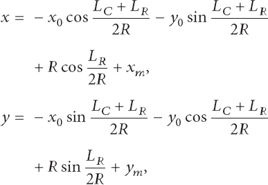
The correcting gaze trajectory was shown in Figure 13. The gaze trajectory is near the road's left-edge line in entering and exiting phases and is far away from it in the middle of the arc curve. Again, there are no intersections between the gaze trajectory and the road's edge line. Compared to the road's centerline, the correcting gaze trajectory's starting point lags behind, its terminal point advances before, and its curvature is greater. The correcting gaze trajectory in the first quadrant can be expressed as follows:
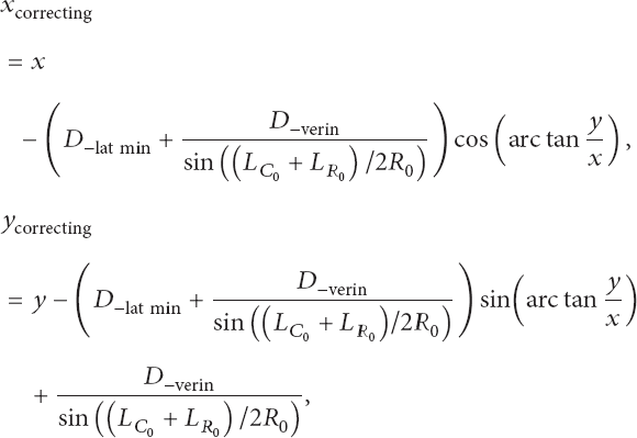
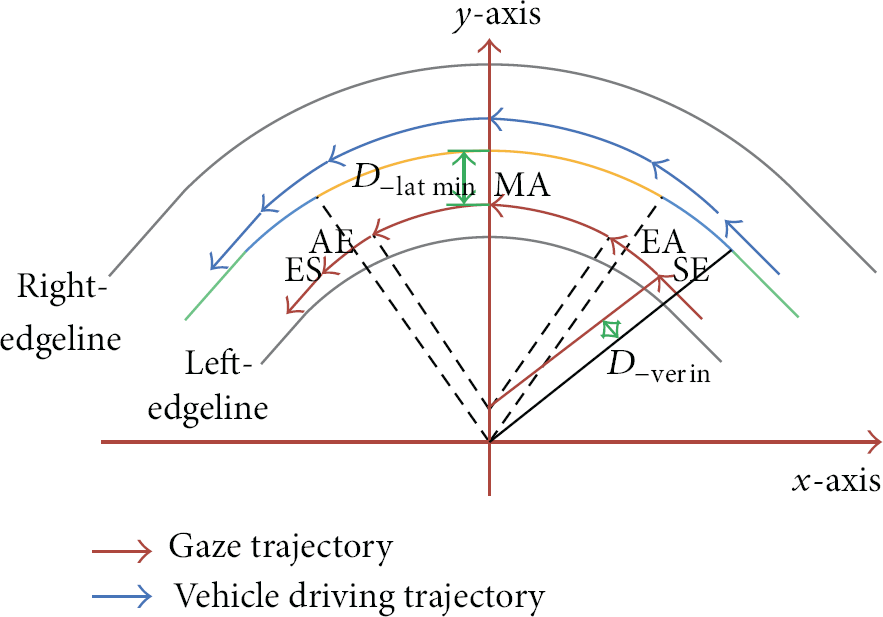
Schematic diagram of correcting gaze trajectory.
where D–lat min is the smallest deviation of the gaze trajectory from the road's centerline. D–verin is the distance between the line connecting the center of the arc of the road's centerline with the intersection of the easement curve and the circular arc and the line connecting the center of the arc of the gaze trajectory with its starting point. (x, y) are the coordinates in the xy-plane of the intersection point in the road's centerline. Again, point (x, y) is in the same ray as point (xcorrecting' ycorrecting).
3.3.4. Cutting Gaze Trajectory
The cutting gaze trajectory was presented in Figure 14. The gaze trajectory is far away from the road's left-edge line in entering and exiting phases, and is near it in the middle of the arc curve. Compared to the road's centerline, the cutting gaze trajectory's starting point advances before, its terminal point lags behind, and its curvature is smaller. The cutting gaze trajectory in the first quadrant can be expressed as follows:

Schematic diagram of cutting gaze trajectory.

where (x, y) are the coordinates in the xy-plane for the intersection point in the road's centerline. Once again, point (x, y) is in the same ray as point (xcutting, ycutting).
3.3.5. Swing Gaze Trajectory
The swinging gaze trajectory was shown in Figure 15. The gaze trajectory is on the right side of the road's left-edge line in the curved section's entering phase and exiting phase. Near the middle of the curved section, the gaze trajectory is located in an uncertain position. Compared to the road's centerline, the swing gaze trajectory's starting point is in advance, the terminal point lags behind, and the curvature is smaller. The swing gaze trajectory in the first quadrant can be expressed as follows:


Schematic diagram of swing gaze trajectory.
where
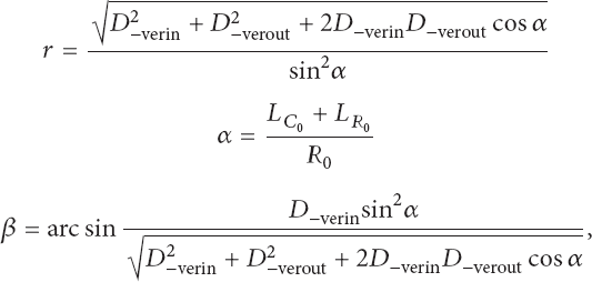
where D–verout is the distance between the line connecting the center of the arc of the road's centerline with the intersection of the easement curve and the straight-line section and the line connecting the center of the arc of the gaze trajectory with its ending point. r is the distance between the center of the arc of the road's centerline and that of the gaze trajectory. α is the angle between the line connecting the center of the arc of the road's centerline with the intersection point of the straight-line section and the easement curve, and the line connecting the center of the arc of the road's centerline with the intersection point of the easement curve and the straight-line section. β is the angle between the line connecting the center of the arc of the gaze trajectory and its starting point, and the line connecting the center of the arc of the gaze trajectory and that of the road's centerline. (x, y) are the coordinates in the xy-plane of the intersection point in the road's centerline. Again, point (x, y) is in the same ray as point (xswing' yswing).
3.3.6. Drifting Gaze Trajectory
The drifting gaze trajectory is shown in Figure 16. The gaze trajectory is on the right side of the road's left-edge line in the curved sections entering phase exiting phase. Near the middle of the curved section, the gaze trajectory is located in an uncertain position. Compared to the road's centerline, the curvature of the drifting trajectory is smaller. The drifting gaze trajectory in the first quadrant can be expressed as follows:
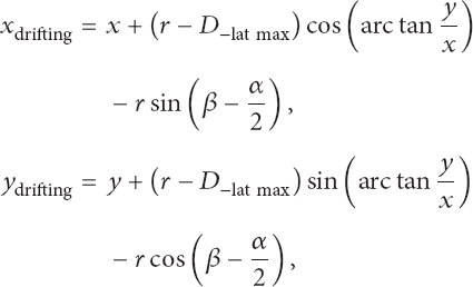
where
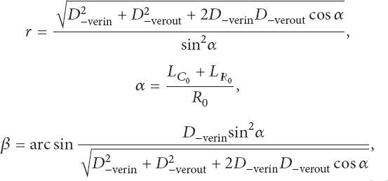

Schematic diagram of drifting gaze trajectory.
where β is the angle between the line connecting the center of the arc of the gaze trajectory and its ending point, and the line connecting the center of the arc of the gaze trajectory and that of the road's centerline. (x, y) are the coordinates in the xy-plane for the intersection point in the road's centerline. Again, point (x, y) is in the same ray as point (xdrifting, ydrifting).
3.4. Discussion
It had been verified by many researchers that the driver's gaze points are distributed in the region close to the road kerb, and several computational models had been proposed to explain this phenomenon. However, there is still no consensus on whether the actual gaze target is the tangent point itself—or some other road point in its vicinity—or on what the functional significance of the gaze points' distribution during curve driving might be.
In this paper, experimental investigations have found that the gaze trajectory is parallel to the vehicle's driving trajectory, and types and models of gaze trajectory have been derived based on the research on vehicle driving trajectory. It is quite apparent that the gaze trajectory will be determined by the distance offsets between the gaze trajectory and the road's centerline in the curved sections entering and exiting phases, as well as the middle part of the curve. Combined with the discovery that gaze points are always distributed in the region close to the road edge, the following conclusions can be deduced.
Some subjects' gaze points follow the change in road alignment quite well, and the starting and terminal points of the gaze trajectory are in the same rays as those of the road's centerline. In this case, the gaze trajectory coincides with the road edge, such as in the ideal gaze trajectory.
In other cases, the gaze points follow the change in road alignment in general, but the starting point of the gaze trajectory lags behind or is in advance of that of the road's centerline. Hence, a distance offset between the gaze trajectory and the road edge exists, and the offset is not a constant value, varying in different sections of the road. All gaze trajectories except for the ideal type belong to this form.
Under the assumption that the gaze trajectory starts at the same radial point as that of the road alignment, the driver can obtain information from the road edge about the road alignment and curvature so as to steer the vehicle appropriately. Therefore, there is no adjustment in gaze trajectory made by the driver during the whole turning process, and the gaze trajectory coincides with the road edge. During this time, the vehicle's handling stability can be either good or bad.
When the gaze trajectory starts in advance of or behind the road alignment, the information the driver obtains visually cannot completely reflect the road alignment and curvature. In other words, the road alignment the driver obtains visually does not match with the expected one. Thus, continuous correction is needed. Due to differences in psychology, driving experience, information processing mechanism, and so forth, from one subject to another, different types of gaze trajectory and corresponding driving trajectories were generated in the experiment, leading to differences in vehicle handling performance.
Drawing on the above analysis, it is known that where the gaze trajectory starts from and how the driver adjusts his/her gaze trajectory on curves are the two salient factors that impact the terminal gaze trajectory and the vehicle's driving trajectory, as well as the vehicle's handling stability.
4. Conclusions
When driving along a winding road, eye movements and vehicle steering are tightly linked. Much research has been done to investigate the relationship between the distribution of fixation points and the vehicle steering angle in curves driving. Until now, there had been no consensus on where the gaze targets are located and what the functional importance of the distribution of gaze points might be.
Therefore, research similar to the prior work was executed in this paper. Drivers' visual behavior was measured while driving around right- and left-hand curves. Motorway on-ramps and interchanges were picked out as the road sections to be analyzed. Hence, the impact of traffic flow on the driver's visual activity could be ignored and the road alignment would be the only impact factor. To eliminate the influence of regional differences, the test was carried out in three representative cities, and urban inhabitants were employed to drive the test vehicle on the appointed routes in each city.
According to the distribution density of gaze points of all participants, it was deduced that the driver's area of interests when driving around a curve is located on his/her left side, which means that the driver pays attention to the inner road edge on left turns and the outer road edge on right turns. Furthermore, the heights of the gaze targets hardly changed. A further investigation discovered that the gaze trajectory was parallel to the vehicle's driving trajectory on these one-way curves. Based on prior research on vehicle driving trajectories, six types of gaze trajectory were derived, and models for each type were established.
Combining the discovery that gaze points are always distributed in the region close to the road edge with the models of gaze trajectory, it was deduced that the starting point of the gaze trajectory has a salient influence on the driver's gaze trajectory on curves and thus on the vehicle's driving trajectory and handling stability. When the gaze trajectory starts at the starting point of the road's centerline, the gaze trajectory will coincide with the road edge and there will be no adjustment during the turning process. In the case where the gaze trajectory lags behind or is in advance of the road's centerline, continuous correcting of the gaze trajectory is carried out, which leads to different types of gaze trajectory and vehicle driving performance. Therefore, the starting point of the gaze trajectory has great significance for the gaze trajectory and vehicle driving trajectory. In future research, more focus should be placed on how the starting point is determined and what factors influence its position.
Conflict of Interests
The authors declare that there is no conflict of interests regarding the publication of this paper.
Footnotes
Acknowledgments
This research is supported by the National Natural Science Foundation of China (Grant nos. 51208225 and 51375200). The authors wish to thank KingFar International Inc. Technology Center for providing the FaceLAB device and professional suggestions on experimental design.