A Component-Based Modeling and Validation Method for PLC Systems

Abstract

Programmable logic controllers (PLCs) are complex embedded systems that are widely used in industry. This paper presents a component-based modeling and validation method for PLC systems using the behavior-interaction-priority (BIP) framework. We designed a general system architecture and a component library for a type of device control system. The control software and hardware of the environment were all modeled as BIP components. System requirements were formalized as monitors. Simulation was carried out to validate the system model. A realistic example from industry of the gates control system was employed to illustrate our strategies. We found a couple of design errors during the simulation, which helped us to improve the dependability of the original systems. The results of experiment demonstrated the effectiveness of our approach.

1. Introduction

Programmable logic controllers (PLCs) are widely used in industry for safety critical embedded systems. A PLC controls several physical plants concurrently. It receives signals from sensors and human inputs and produces control commands to actuators cyclically. A PLC embedded software system is different from conventional software. It is a reactive system that is designed for nonterminating work. The environments are always uncertain and changing with time. Some of the control requirements are real-time related. All of these issues make it hard to ensure the safety and reliability of the control system. Validating such systems is of paramount importance because they are widely used in industrial applications and must meet stringent safety requirements.

Several formal techniques are used to model and analyze PLC-based embedded systems. Most studies on PLCs have focused on PLC program modeling and verification. Mader [1] has presented an overview and classification of PLC models. Canet et al. [2] directly coded the existing program written in instruction list (IL) language into the input language of the SMV [3] model checker. They did not consider the aspect of time in the model. The Petri net is also a well-known method of modeling PLC systems. Heiner and Menzel defined a Petri net semantics of IL in [4]. Programs and environments were modeled as the Petri net. But the verification phase has not been considered. In [5, 6], the signal interpreted Petri net (SIPN), which extended the Petri net with input and output signals, was adopted to model PLC systems. Such extension is powerful for modeling, but the Petri net tool is not strong enough to analyze the SIPN. None of the above studies are component based. As PLC system always has time constraints, timed automata were adopted to model this feature. A PLC program translation tool is given in [7]. It translates IL programs to timed automata that can be checked by Uppaal [8]. But the types of data are restricted to the Boolean type. Zhou et al. [9] proposed a more complete method than current ones of translation from IL program to timed automata. The translation is efficient which results in a reduced verification model. Wang et al. [10] used timed automata to model the PLC control software and environments and then systematically verified the functional and timed properties. A framework for specifying and verifying control logic components in industrial applications is proposed in [11]. The component includes specification and implementation and can be automatically translated into inputs of SMV.

Validation using formal methods suffers from well-known complexity limitations. The modeling languages are not expressive enough to faithfully describe the actual behavior by using real-time constraints. Furthermore, validation by fully exploring the state space is prohibitive, as the model involves data and timing constraints. Timing constraints are necessary for analyzing the dynamic behavior and drastically increasing the complexity of the state space. Our modeling and validation method can avoid these shortcomings. In this paper we apply a new model construction methodology to PLC applications. The component concept is first employed in the PLC modeling area. The BIP [12] framework supports component-based modeling and validation. The BIP framework enforces the reusability of functional components. We propose a components library of the commonly used functions and a general architecture for device motion control system. The architecture decomposes the controller into three levels. Each level is modeled as a composition of functions. As the modeling and validation focus on the system level, we not only model the control software but also model the environment and human behavior. Environmental uncertainty is expressed in our model. As the system is very complex, we validate it by simulation. Requirements are formalized as monitors, composed of the global system model. The monitored system was extensively simulated in BIP. The simulation was carried out by BIP tool chain. We found and corrected two design errors that may correspond to bugs in the real system.

This paper is organized as follows. Section 2 gives background on the BIP framework and associated tools. Section 3 presents the architecture and components library. Section 4 contains the case study. The validation work is shown in Section 5. Section 6 concludes the paper.

2. The BIP Framework

The BIP (behavior-interaction-priority) component framework is a formal supporting, rigorous design for heterogeneous component-based systems [13]. It allows the description of systems as a composition of atomic components characterized by their behavior and their interfaces. It supports a system construction methodology based on the use of two families of composition operators: interactions and priorities. Components are composed of the layered application of two operators.

In BIP, atomic components are finite-state automata extended with variables and ports. Variables are used to store local data. Ports are action names and may be associated with variables. They are used for interactions with other components. States denote the control locations at which the components await interaction. A transition is a step, labeled by a port, from one control location to another. It has an associated guard and an action that are, respectively, a Boolean condition and a computation defined on the basis of local variables. Connectors include sets of ports and interactions. Interactions describe synchronization constraints between the ports of the composed components. Interactions are used to specify multiparty synchronization between components as the combination of two protocols: rendezvous (strong symmetric synchronization) and broadcast (weak asymmetric synchronization). Interactions are defined using connectors. Every interaction has a guard, that is, an enabling condition and an action. The action can be an update function, operating on data associated with the ports participating in the interaction. Connectors are sets of ports augmented with additional information as follows. Within the connectors, every port is either a synchron or a trigger type of port. Trigger ports are used to initiate broadcasts; that is, any subset of ports containing at least one trigger port denotes a valid interaction of the connector. Rendezvous synchronization is obtained on connectors where all ports are synchrons. For such connectors, the only valid interaction is the maximal one, that is, the whole set of ports. Finally, connectors provide mechanisms for dealing with data associated with ports of interacting components.

The BIP framework is concretely implemented by the BIP language and an extensible toolbox [14]. The toolbox provides front-end tools for editing and parsing BIP programs, as well as for generating an intermediate model, followed by code generation (in C++) which is used for runtime validation. The correctness of the generated C++ code is confirmed by the formal semantics of BIP. Intermediate models can be subject to various model transformations focusing on the construction of optimized models for sequential [15] and distributed execution [16]. It also provides back-end tools including runtime for analysis (through simulation) and efficient execution on particular platforms. The toolbox provides a dedicated modeling language for describing BIP components and connectors. The BIP language leverages on C-style variables and date type declarations, expressions, and statements. It also provides additional structural syntactic constructs for defining component behavior, specifying the coordination through connectors.

3. The Component-Based Modeling Method

One of the advantages of the component-based modeling method is reusability. A system architecture and a component library are ways to achieve reusability. Motion control systems use PLCs to control the movements of mechanical devices that are powered by motors. The common parts of these systems are the functional control of all kinds of motors. Motors include constant speed motors and variable speed motors. Some devices are required to reach an exact position. Some require the devices to stop when meeting the limit switch. In particular, BIP separates behavioral and architectural aspects in modeling. Architecture is meaningfully defined as a combination of interactions and priorities. In addition, we discuss the expressivity of BIP and related component-based frameworks. In our discussion, we show that the combination of interactions and priorities gives BIP a universal form of expressiveness. Numerous translations are defined from existing models of computation and domain-specific languages into BIP.

3.1. System Architecture

The global architecture of the BIP model is shown in Figure 1. This architecture is general and suitable for motion control applications. When we model the system with a component concept, we adopt the following decomposition principles.

1. The software and hardware architecture partition is as follows. The architecture design can construct the system topology relations. The system run environment also has an impact on the partition. We first consider the natural physical organization. The system is decomposed into user, software system, and controlled devices.

2. Layered decomposition of the control software is as follows. In a PLC-based control system, the control software is organized as layers. The lower layer supplies services to the upper layer. The top layer is responsible for user interaction and operation flow. Different domains have different meanings. For example, the top layer of the motion control system manages scenario control. The middle layer is always a protocol. The bottom layer is the functional level, which takes charge of the interaction and controls the actuators and sensors.

3. The functionality decomposition of each layer is as follows. The father principle can follow a business step or function modular. For example, the first level is decomposed into the command scheduler and scenario components. This will enforce the reusability of the scheduler. The bottom layer is composed of individual functional components.

Figure 1:

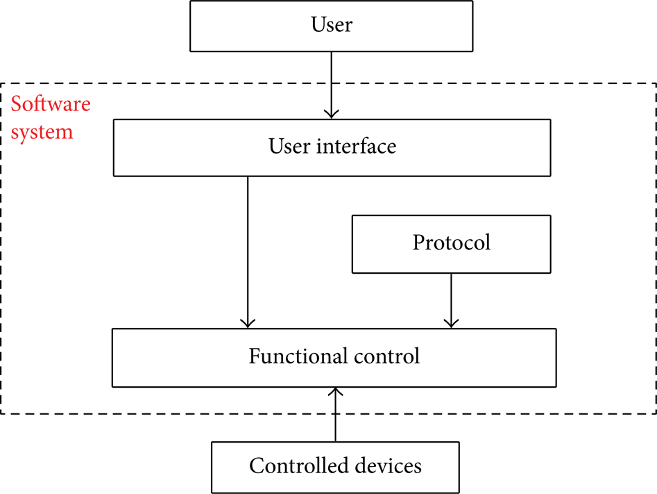
The architecture of the PLC motion control system.

3.2. Component Library

3.2.1. Motion Control Components

Motion control systems always have similar basic functions. We summarize and model these functions in the library. When modeling and verifying other motion control systems, the system architecture and components in the library can be adopted directly to compose the system model. We formalize four kinds of frequently used control functions as follows:

• ConSpeedControl(DevNo, Dir): controller for constant speed devices with a limit switch.

• ConSpeedControl(DevNo, Dest): constant speed device controller for accurate destinations.

• VarSpeedControl(DevNo, Speed, Dir): controller for variable speed devices with a limit switch.

• VarSpeedControl(DevNo, Speed, Dest): variable speed device controller for accurate destinations.

DevNo is the name of a controlled device. Dir is the moving direction and Dest means the destination. A model of a ConSpeedControl(DevNo, Dir) component is shown in Figure 2. When receiving the start command from the main program, the component moves to ST1 state and then notifies the Constraints Checker component of the current position of the device. Then, the component waits at FN1 for some time. After that, it sends the move command to the device component cyclically. In each cycle, it asks the Constraints Checker if the movement is permitted. It moves as long as the answer is YES. The control flow returns to the initial state if the device reaches a limit switch during the movement. Five states of the model can handle the preStop signal and move to the SP1 state.

Figure 2:

The model of the constant speed controller.

3.2.2. Device Components

There are two kinds of devices for motion control systems: constant speed devices and variable speed devices. In the library for motion control, we have the VarSpeedDev(Dir) component and the ConSpeedDev(Dir, Speed) component.

The VarSpeedDev(Dir) components in Figure 3 are used to model the physical properties of variable speed devices. When the model receives a move command from the VarSpeedControl component, it moves to the start state and then regulates the speed (according to the specified speed) at every tick time. When a limit is reached (either the UP_LMT or the DOWN_LMT), the device throws a signal that informs the VarSpeedControl that the device has reached that limit. The moving() and slowdown() functions are used to model the motion of the device. A random factor is added in every single moving step to model uncertainty. moving() is executed when the move command is received, while slowdown() is executed when no move command is received and the device keeps moving due to inertia.

Figure 3:

The model of the variable speed device.

4. Case Study

4.1. Application Description

The case presented in this paper is a real industry application used in LingShan Buddhist Palace of Jiangsu province, China. This system was developed from 2006 to 2008 and continued running for four years. The control software consists of nearly 10000 lines of PLC code. A round stage is located in the Buddhist Palace. There is a cycle of steel track around the stage. Eight gates moving on the track in a queue can turn the stage into a closed round space. A gate warehouse is located near the stage. All gates can fold in the gate warehouse when they are not in use.

The main functionality of the PLC system is to control the folding or unfolding of the gates into or from the gate warehouse and move along the steel track. The physical structure of this system is presented in Figure 4. A user can give commands in the control panel, and the PLC will execute the commands and sends electric signals to physical devices through PROFIBUS-DP network. The speed, location, and status of the devices are sent back to the PLC. The gates are 20 m long, 19 m high, and 1.2 m wide. They are made of wood and are very heavy. The gates have wheels at the bottom, so that they can slide along the track. Eight gates are stored in the gate warehouse. Only six of them can emerge from the gate warehouse and move along on the track. The last two emerge directly to their final (and fixed) position. Gates standing on a seat are pulled by push-pull units when they move straight into the gate warehouse. Two lifting platforms are used to lower or lift the seats of the gates. Each lifting platform is fixed with four latches. The latches are driven by constant speed motors. There are two limit switches at the end of each latch. Only when a latch is completely inserted or pulled out will the switches be able to send high-level signals to the PLC. In the folding or unfolding process, each pair of gates requires seven steps, and three pairs require a total of twenty-one steps. These steps are described below.

1. At first, Gate 7 and Gate 8 standing on the lifting platform and the track on the lifting platform are connected to the track on the steel cycle. The two gates move on the track in parallel to position 20500 mm. There are no gates on lifting platforms.

2. The lifting platform should move down and free up the space for Gate 5 and Gate 6. Because lifting platforms are fixed by latches, we should pull out eight latches. In order to pull out the latches, the lifting platforms have to move up 10 mm to make the latch movable.

3. Eight latches are then pulled out.

4. The lifting platforms get down to −790 mm to free up the space for Gate 5 and Gate 6.

5. Then the eight latches of the lifting platforms are inserted.

6. The lifting platforms get down to −798 mm to make the latches stick.

7. The push-pull units pull all of the gates forward by 2378 mm and slow down to meet the limit switch. Then the seats of Gate 6 and Gate 5 are connected to the track on stage.

Gate 6 and Gate 5, together with Gate 7 and Gate 8, move forward to 20050 mm. The process is then repeated. The moving of Gate 3 and Gate 4 is nearly the same. If the gates are already surrounding the stage, the PLC system controls the movement of the gates into the warehouse, pair by pair. In the folding (backward) scenario, the steps are carried out in the opposite order.

Figure 4:

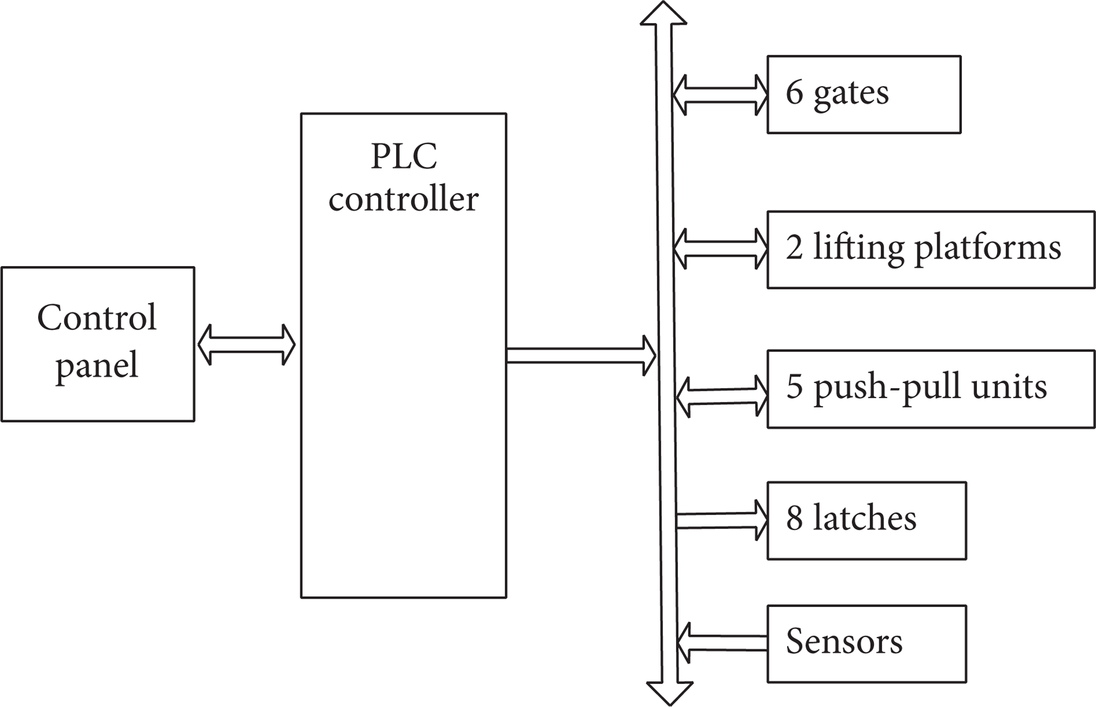
The physical structure of the PLC control system.

In this system, human safety is of most importance. The gates, push-pull units, and lifting platforms are big and heavy. They move within a restricted space. Some of their motion routes cross. We should ensure that these devices do not crash into each other. There is an urgent stop button on the control panel. When something dangerous happen, a user can press the stop button and stop all devices within 0.1 s. The functional requirements include the following.

• If the moving device meets the limit switch, it should stop immediately.

• If the user presses the stop button, all devices should stop within 0.1 s.

• A moving device must not exceed its upper or lower bounds.

4.2. Component-Based Modeling of the PLC System

The software is the most important part. There are hundreds of devices moving in a restricted space that need to be controlled. Thus the kind of software that is required is complex. Based on the proposed general architecture for a motion control system, we built a distinct layered structure for this system shown in Figure 5.

• The top level is the main program. It stores the scenario information, executes user commands, and schedules the device controllers. The main program receives forward, backward, or uStop commands from the user and executes control sequences. It starts moving devices one by one with the preset order. The user can stop the scenario and restart the process with two direction choices (forward or backward).

• A constraints checker is in the middle which controls the proper execution of devices based on the safety constraints. It receives status data from all devices and checks whether the device can move or not. It stores status data of all devices.

• The bottom level, close to the physical environment, is the functional level. It includes four kinds of device controllers, respectively, the atch controller, gate controller, push-pull unit controller, and lifting-platform controller. If a device is required to move, it requests permissions from the execution control level. The latter checks the safety constraints and responds accordingly to the controller. Every time the data of a physical device changes, the controllers update the data of the execution control level. After a device moves to its preset destination, the controller sends a finish signal to the main program. The main program will start moving the next device and so on, until the whole scenario is completed, that is, when all devices reach their positions.

Figure 5:

The architecture of the PLC control system.

4.2.1. Main Program

The main program level in Figure 6 executes the scenario and user commands. In order to increase the reusability of the system model, we separate the operations and scenarios into two components. With this structure we can add new scenarios without changing the schedule component. In the initial state of the schedule component, it receives forward or backward commands from the user and then transits to the RUN state. The user may press the stop button (uStop) during the execution of scenarios. The uStop command will stop all the devices in the system. The component will transit to STOP state. A singleDevStop port is connected to each preStop port of all device controllers with strong synchronization. The allStop of scheduler, the stop of scenario, and the stop of all device controllers are globally synchronized. After all devices move to preStop states, the scheduler component goes back to the INIT state. The user can continue with forward or backward command. After the whole scenario is finished, the model comes back to the INIT state.

Figure 6:

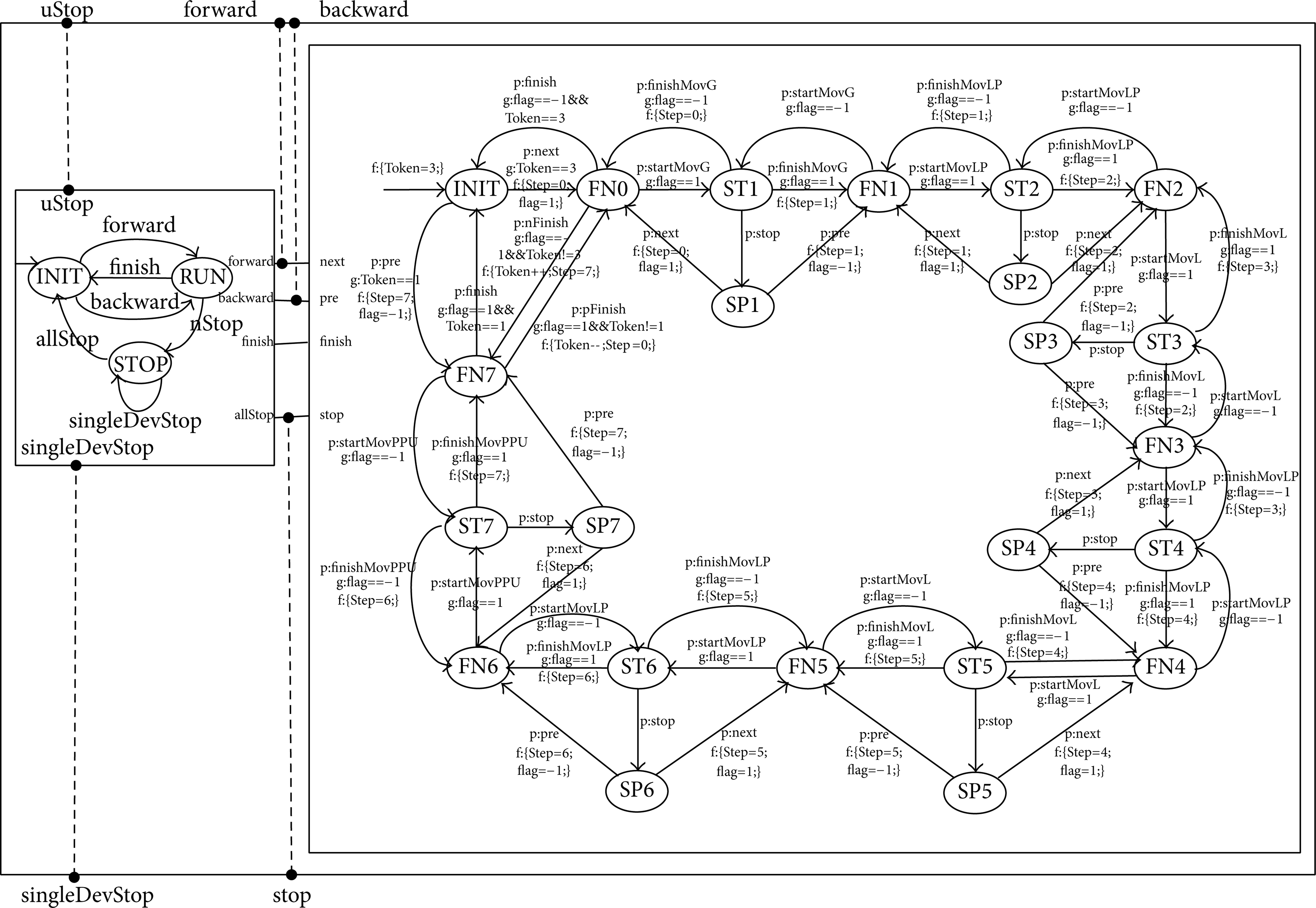
The model of main program.

There are three cycles in the scenario component. Every cycle is the control process of a pair of gates. The variable Token is used for the cycle number. The variable flag indicates the two directions. Seven steps are required to move a pair of gates. Therefore, every cycle contains seven pairs of starts to move a device and complete the move. Every single step corresponds to a device control on the functional level. Every step can handle a stop event from a schedule component. The model transits to a stopstate and waits for the forward or backward command.

4.2.2. Constraints Checker

The model of the Constraints Checker in Figure 7 is very simple. If data is changed in the controllers, it receives a notify signal and renews the data by using the UpdateData() function. If controllers ask for permission to initiate a movement, the constraint() function calculates the result and sends it back to controllers. The constraint() function written in C-like language comes from the source code of this control system.

Figure 7:

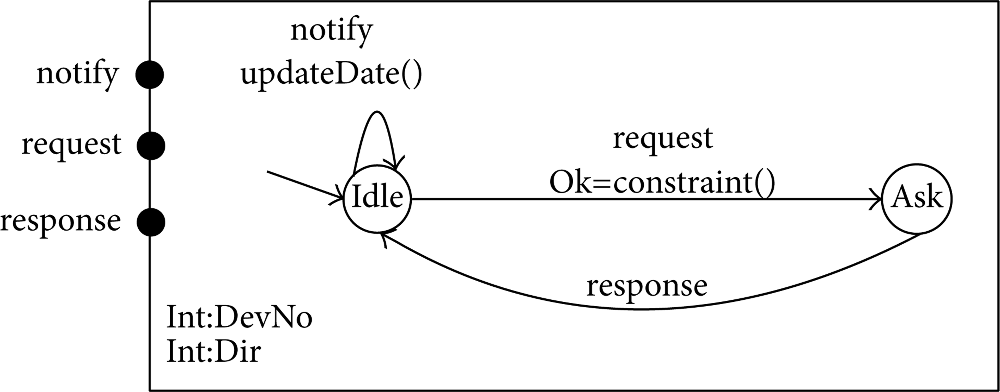
The constraints checker model.

4.2.3. Functional Component

The controller models of the gate, push-pull unit, and lifting platform are all instances of the VarSpeedControl(DevNo, Speed, Dest) component type. The controller models of the latches are instances of the ConSpeedControl(DevNo, Dir) component type. In this application, we have six gate controllers, eight latch controllers, two lifting-platform controllers, and 5 push-pull unit controllers.

4.2.4. Environment Model

In order to make this system a closed one, we model the controlled devices and the user in the environment. Latches are instances of ConSpeedDev(Dir) components. The gates, push-pull units, and lifting platforms are instances of VarSpeedDev(Dir, Speed) components.

In order to simulate the behaviors of a user, we design a random user model. The random user in Figure 8 makes a decision every 30 ticks by choosing forward, backward, uStop, or nothing with a random rate. This model tries to model all possible behaviors. This ensures that the controller acts correctly not only in the case of normal behavior but also when unexpected behavior occurs.

Figure 8:

The model of user.

In this case, we have the PLC codes. The BIP model should be a correct abstraction of the codes. The software has the corresponding part with BIP component, but the correspondence is not exactly the same. For example, the gate control function in the PLC code calls for several subroutines. We model these subroutines in one component. But they are functional equivalents. Regarding specific data and operations in the BIP model, we obtained these directly from the PLC code in the following way.

• All relevant data (blocks) in the PLC source code are translated directly into local variables (of particular components) of the BIP model.

• Similarly, functions (blocks) in the PLC source code have been translated directly into C functions and have been called within transitions in the BIP components.

For this case study, the system model contains 46 atomic components and 185 connectors (interactions). The system is a compound component. The BIP script of the system consists of more than 2200 lines.

5. Validation

Validation of BIP models can be achieved by using runtime validation techniques. The runtime validation technique for BIP is based on the construction and execution of monitored systems. Historically, the validation approach is oriented towards finding errors rather than proving the absence from design. This approach has been adopted for BIP components as explained in [17]. It consists of constructing an executable model for evaluating safety requirements. Monitors are atomic components that observe the system state and react by moving to the error state where the safety properties are violated, that is, if an interaction has been executed or an invalid sequence of interactions has been executed. The BIP framework provides native support for building and running executable models for monitored systems.

Here we use the runtime validation of BIP, as the model is complex and constrains 2000 lines of C code in the constraint component. The runtime validation technique needs to construct and execute the monitored systems. The requirements are modeled by monitors that are atomic components. Monitors continuously sensor the state of the system. Reaching an error state means a violation of some requirement. The principle of the validation of a global model M by using monitors is as follows.

• Assume that we have n properties to verify P = {p₁,…, p _n }. For each property p _i , construct a monitor m _i (as a component in BIP) that observes the behavior of M and reports errors if M behaves incorrectly.

• Compose all of the monitors m _i and the global system model M to obtain the monitored system, say,

$M^{\prime }=M\parallel m_{\mathrm{1}}\parallel \cdots \parallel m_n.$

(1)

Now, the model M′ is ready for simulation. If the requirements are violated, the monitors will transit to the error state.

5.1. Modeling Requirements as Monitors

Four requirements are modelled as monitors. When this requirement is violated, the monitor transits to the ERROR state.

5.1.1. Deadlock-Free Property

The reactive embedded system should make rapid response to the input of the environments and executed infinitely. So the system should be deadlock free. For this property we do not need to build monitors, we run the BIP tool with model M.

5.1.2. Stop Properties

The device will stop if it meets the limit switch. For this property, if the monitor shown in Figure 9 catches the ReachLmt signal, before receiving next start signal, there should be no move signal from the device controller to device. This property concerns 16 devices (i.e., all devices, except for push-pull units).

Figure 9:

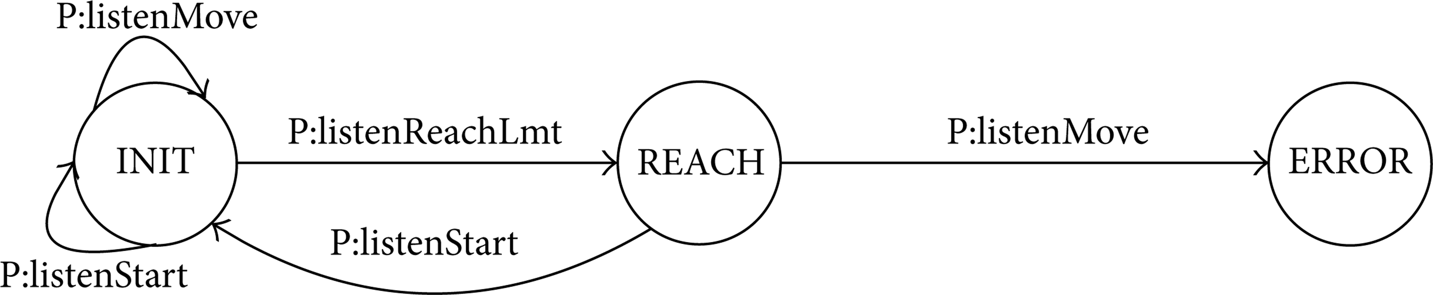
The monitor of stop property.

5.1.3. Urgent Stop Properties

The user stop command should be executed within 1 tick (0.1 s). Figure 10 is the formal model.

Figure 10:

The monitor of urgent stop property.

5.1.4. Safety Bound Properties

Device movement cannot exceed the upper or lower bounds. Every device has the travel range, so 21 monitors are built for observation. From the INIT state, after a tick time, the monitor of Figure 11 gets the current position of the device. At the CHECK state, if the current position is less than the low bound or bigger than the upper bound, this monitor will transmit to ERROR sate and print LIMIT_MONITOR: ERROR; otherwise it will transit to the INIT state. A different instance of this monitor has been used for every moving device in the system.

Figure 11:

The monitor of safety bound property.

5.2. Validation Result

The BIP model M′ can be compiled to a program written in C++ by the BIP tool and then can be further compiled to an executable binary program. We ran the simulation program for seven hours, which corresponds to approximately four hours of a real system's lifetime. We discovered two design errors for the two types of users.

5.2.1. Validation of Stop Property

The first versions of the system model do not satisfy stop properties. The reason for this is that the limit position is reached if the position of the device is within a fixed range of the limit position. This is the case in physical deployment, where limit switch sensor checks if the device is near the sensor. In the linear case, assume that sensor is located at x and that it checks if the device is in the range of [x − c, x + c]. The sensor sends the result every cycle, and each cycle takes δT time. If the speed parameter is not properly set, for example, the device is asked to move at a speed which is greater than 2c/δT. Then the sensor may fail to detect if the device has reached the limit position. Engineers have confirmed that they have actually experienced this kind of problem. Their speed parameters are chosen by test conducted on the real system. Our simulation can help in choosing the proper parameters.

5.2.2. Validation of Urgent Stop Property

For the urgent stop property, we checked that the stop command takes effect within 1 tick. However, if the property is specified as one in which the stop command takes effect immediately, the simulation will fail. We investigated this situation and found that the stop command is a global command. It is possible that, at the time that user pressed stop, some device, say d₀, has just sent a move command. In the model, a move is followed by a tick. This is intuitively correct because a movement takes some time. Then, the controller can capture the stop command after this tick. Consider

$\cdots \hspace{0.17em}⟶\hspace{0.17em}{d}_{\mathrm{0}}·move\hspace{0.17em}⟶\hspace{0.17em}tick\hspace{0.17em}⟶\hspace{0.17em}{d}_{\mathrm{0}}·preStop\hspace{0.17em}⟶\hspace{0.17em}\cdots .$

(2)

In general, the simulation finds two potential errors in the system. The simulation on computers can also help engineers to choose the proper parameters instead of running experiments in the real world.

6. Conclusion

The paper reports on a component-based modeling and validation methodology for a type of control system implemented on PLCs. We have shown that, by using the BIP component framework, a complete model of the system can be obtained with the help of system architecture and component libraries. We propose a universal software architecture and components library for device motion control systems. The decomposition of the architecture into three layers enhances the readability of the model and allows its complexity to be mastered. Modularity is essential for incremental construction and modification. The library can offer commonly used components. This makes the modeling of such a control system convenient and dependable. Timing constraints are modeled by using a time progress signal tick in each component that represents the progression of time by one unit. The tick signals of all components are strongly synchronized.

We have presented a rigorous method for validating the global system model by simulation. The method consists of building a monitored system where the requirements are modeled by monitors that continuously sense the state of the system to be validated. Reaching an error state means the violation of some requirements. Following the BIP design flow, the following work is about the model based code generation. Although the BIP toolkit has the code generation subpart, it is for the generation of C++ code. The generated code cannot be used at all. We are developing a code generation algorithm and tool for the PLC hardware platform. The special features of a hardware platform should be considered.

Conflict of Interests

The authors declare that there is no conflict of interests regarding the publication of this paper.