
Abstract
In this paper, a novel thin-disc piezoelectric actuator, 4-9-9-14 piezoelectric actuator, is used to construct and drive the micro/nanometer level biaxial piezoelectric actuated stage. The 4-9-9-14 piezoelectric actuator offers a better balanced capability of forward rotation and reverse rotation than the conventional edge-driving piezoelectric actuator. The biaxial piezoelectric actuated stage structure comprises a base, a V-shaped guide rail, an optical scale measurement system, a preload adjusting structure, and a load-carrying stage. The movement signals of the piezoelectric actuated stage are read and analyzed by means of NI PCI-6115 data acquisition card and LabVIEW software operating in conjunction with a linear optical scale. The new consideration of tuning Ton time is used in place of the traditional method of changing the magnitude of driving voltage to control the stepping distance of the stage. A combined driving signal is based on the sum of a continuous driving signal for Ton time and a DC signal for Ton time; the combined driving signal is continuously output in this manner to form a continuous driving pulse chain. Under a constant driving voltage, the displacement of the stage increases with Ton time and the displacement of the stage decreases with Ton time.
1. Introduction
Due to technological advancements, a wide variety of motors are in use in different fields. Motors nowadays are no longer restricted to those driven by an electromagnetic force, as an unorthodox type of motors, namely, piezoelectric ultrasonic motors (or known as piezoelectric motors for short), has emerged thanks to the rapid development of material technology in recent years. A linear mechanical mechanism is used to perform linear translation mostly by a conventional rotary motor that operates in conjunction with ball screws. However, ball screws are flawed with backlash and thus are not effective in enhancing positioning precision and speed. By contrast, piezoelectric motors have advantages over conventional rotary motors. For example, piezoelectric motors feature a larger holding torque and less instability (i.e., the driven mechanism keeps moving under inertia) than conventional rotary motors. Due to its aforesaid advantages, a piezoelectric motor is capable of precise positioning. Other advantages of piezoelectric motors include insusceptibility to an electromagnetic field, high-precision positioning, low noise (because their deceleration mechanism can work without any gear), compactness, low weight, and large torque [1–3].
In recent years, a piezoelectric motor poses a new choice of actuators in terms of precise stage positioning. In engineering-related application, stage movement precision technology has a trend toward sophistication, miniaturization, high precision, and high stability and has a strict requirement for precision and stability of a driving device in particular. Hence, piezoelectric motors still have much room for development when functioning as actuators for driving stages.
Most piezoelectric motors employ a stacked/multilayered piezoelectric material or an alternate polarization of electrodes of piezoelectric material. These piezoelectric materials are expensive, and thus commercially available piezoelectric motors are expensive, too. A piezoelectric motor developed by our research team is a 4-9-9-14 piezoelectric actuator that comprises an inexpensive piezoelectric buzzer. The purpose of the piezoelectric actuator is to position a stage in a mechanical system in a manner that the movement and positioning of the state can be controlled by varying the driving frequency, driving voltage, and driving duration of the piezoelectric actuator [4].
The 4-9-9-14 piezoelectric actuator comprising a buzzer, as disclosed in this paper, applies to a biaxial piezoelectric actuated stage designed by our research team. Considering the nonlinearity of piezoelectric materials, our research team controls the actuator with a continuous driving pulse chain by adjusting the driving duration by a constant driving voltage, evaluating the characteristics of the 4-9-9-14 piezoelectric actuator, adjusting the driving voltage to stabilize stage characteristics, and constructing a controller adjustment parameter in accordance with a characteristic measurement experiment.
Due to advancement of semiconductor technology and robust development of computer technology, not only are PC-based measurement systems available today, but also an era of virtual instruments is beginning, thereby speeding up a design process and providing flexible functions. In this regard, LabVIEW and Matlab are most widely used. In this regard, the NI LabVIEW graphic monitoring program and the NI PCI-6115 multifunction data acquisition (DAQ) card used in the experiment are the most appropriate; hence, our research team designs the system required for this paper by LabVIEW. A further objective of this paper is to evaluate the performance of the piezoelectric actuator in stage positioning and design a controller according to the performance thus evaluated.
2. Piezoelectric Actuator
The piezoelectric actuator described in this paper is a thinned piezoelectric actuator designed in an unorthodox way and made from a commercially available inexpensive piezoelectric buzzer (OBO-TE41208-21) [5, 6]. The piezoelectric buzzer consists of a piezoelectric ceramic membrane and a thin metal plate which are glued together by silver paste. The piezoelectric buzzer is intrinsically characterized by that its radial-direction displacement vibration amplitude variation is larger than its longitudinal-direction (or axial-direction) displacement vibration amplitude variation; hence, if the piezoelectric buzzer is designed to be a mechanism for driving a rotor by radial-direction displacement vibration amplitude variation, its various characteristics will be improved. Therefore, our research team develops an edge-driving type piezoelectric actuator [7–9], and its stator structure is shown in Figure 1.

Static structure of 3-4-5 piezoelectric actuator.
In the stator structure of the edge-driving type piezoelectric actuator shown in Figure 1, three round holes of a diameter of 2 mm each are cut out of a metallic (nickel alloy) back panel of the piezoelectric buzzer, arranged in their respective orientations of 90°, 120°, and 150°, and locked with screws, respectively, so that the piezoelectric buzzer appears in the form of an angularly unbalanced (or asymmetric) 90°-120°-150° structure (also known as 3-4-5 structure for short). The actuation principle of the edge-driving type piezoelectric actuator depends on the aforesaid asymmetric 3-4-5 structure and involves converting compulsorily a voltage signal sent to between a piezoelectric ceramic material and the metallic back panel into a deformation wave motion comprising a mixture of a standing wave (displacement extension produced axially) and a traveling wave (displacement extension produced radially); hence, the edge-driving type piezoelectric actuator can be regarded as a hybrid type piezoelectric actuator. As shown in Figure 2(a) [10–12], ANSYS simulation reveals that radial and rotational distortion vectors of leftward (counterclockwise) motion occur at a peripheral position in the 90° sector, indicating that they are capable of driving the rotor to rotate clockwise; no peripheral position in the 120° and 150° sectors is suitable for serving as a driving point of the actuator, because the distortion vectors are attributed to a scattering motion that occurs in the directions of screws located on its two sides. The result shown in Figure 2(b) [10] is consistent with Figure 2(a) except that the distortion vectors at a peripheral position in the 90° sector are rightward (clockwise), thereby indicating that they are capable of driving the rotor to rotate counterclockwise. Switching the edge-driving type piezoelectric actuator between forward rotation and reverse rotation is achieved by alteration of two driving frequencies rather than conventional alteration of a phase difference from a dual-phase driving power source; hence, determination of the forward and reverse rotation driving frequencies of the actuator is of vital importance.
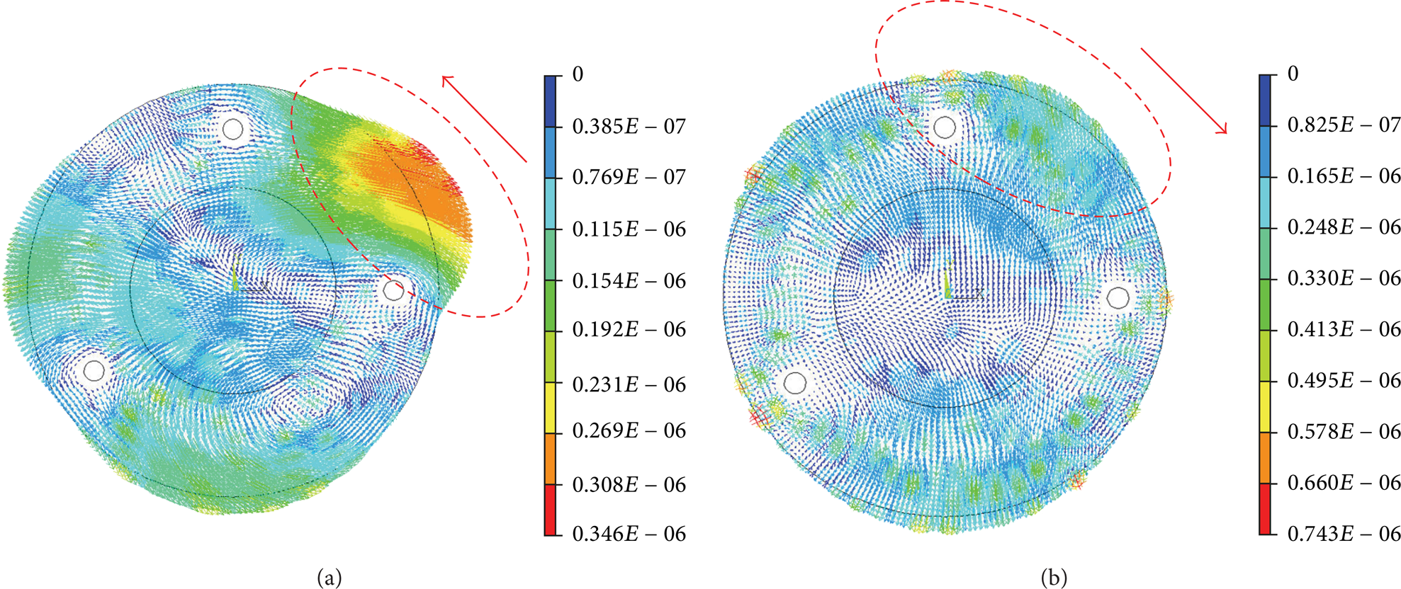
(a) ANSYS dynamic simulation diagram of counterclockwise rotation of the 3-4-5 piezoelectric actuator; (b) ANSYS dynamic simulation diagram of clockwise rotation of the 3-4-5 piezoelectric actuator.
Unlike a conventional piezoelectric actuator, the edge-driving type piezoelectric actuator does not have any alternately polarized electrodes; hence, the forward rotation and reverse rotation of the actuator take place by means of two different driving frequencies (with one being a true resonance frequency of the system and the other being the second-best driving frequency) instead of a phase change (with one phase expressed in sin t and the other phase in − cos t or with one phase expressed in − sin t and the other phase in cos t) of a dual-phase input power source (with one phase expressed in sin t and the other phase in cos t). However, the two different driving frequencies differ from each other in terms of the efficiency of actuation of forward rotation and reverse rotation (strong driving torque and quick rotation in one direction, but weak driving torque and notably slow rotation in the other direction). To overcome the aforesaid drawback, our research team modifies the prototype by balancing the forward rotation and reverse rotation of the piezoelectric actuator, which is achieved by changing its fixation point location and thus modifying the 3-4-5 asymmetric structure and putting four fixation posts on four radii that separate a 40° sector, a 90° sector, a 90° sector, and a 140° sector, respectively, as shown in Figure 3. Therefore, the modified piezoelectric actuator is known as a 4-9-9-14 piezoelectric actuator [10, 13], and distortion vectors of its forward rotation and reverse rotation are depicted in Figures 4(a) and 4(b). The aforesaid modification equalizes the actuation of forward rotation and reverse rotation. The experiment proves that the aforesaid design reduces the difference in actuation between forward rotation and reverse rotation greatly.

Static structure of 4-9-9-14 piezoelectric actuator.
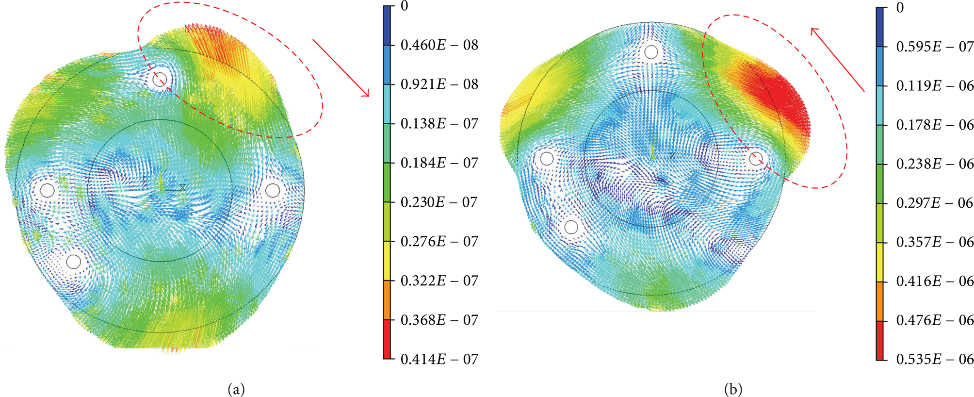
(a) ANSYS dynamic simulation diagram of clockwise rotation of the 4-9-9-14 piezoelectric actuator; (b) ANSYS dynamic simulation diagram of counterclockwise rotation of the 4-9-9-14 piezoelectric actuator.
As shown in the ANSYS dynamic simulation diagrams, it is confirmed that the 3-4-5 piezoelectric actuator and the 4-9-9-14 piezoelectric actuator are equipped with clockwise and counterclockwise actuated capability. A piezoelectric material extends in variable directions; hence, in addition to radial-direction extension, the piezoelectric actuator undergoes axial-direction extension. Afterward, our research team simulates dynamic behavior with ANSYS to effectuate continuous vibration of the piezoelectric actuator and thereby proves that the displacement extension model at the driving position occurs essentially in the form of a radial-direction displacement extension. When a chain of pulse voltage signals are applied to the piezoelectric actuator, the resultant hybrid wave is composed of radial-direction and axial-direction extension distortion. An edge-driving type actuator usually gives priority to radial-direction extension distortion. Radial-direction displacement extension varies with axial-direction displacement extension. Hence, the desirable optimal edge-driving type piezoelectric actuator structure has a maximum radial displacement extension range.
3. Biaxial Piezoelectric Actuated Stage
This paper describes the 4-9-9-14 piezoelectric actuator functioning as a driving device and explains how to design a biaxial piezoelectric actuated stage [14]. A biaxial piezoelectric actuated stage designed by a precise positioning experiment is described hereunder. The biaxial piezoelectric actuated stage structure comprises a base, a V-shaped guide rail, an optical scale measurement system, a preload adjusting structure, and a load-carrying stage [15, 16]. The biaxial piezoelectric actuated stage is divided into an upper stage and a lower stage. Driving is mainly carried out by moving, with the preload adjusting structure, the actuator's stator structure to come into contact with the load-carrying stage such that, upon contact between the actuator's stator structure and the load-carrying stage, the load-carrying stage (upper stage) undergoes linear motion along the x-axis leftward and rightward, and the lower stage undergoes linear motion along the y-axis forward and backward.
The V-shaped guide rail of the biaxial piezoelectric actuated stage is a crossed roller rail that comprises precise rollers which are arranged perpendicularly to each other, held in a holding frame, and intended to travel a 1/2 stroke along a V-shaped groove of the rail, so as to function as a small high-rigidity linear motion system. It features a low sliding friction coefficient, high stability, a low start frictional resistance, high following performance, a large contact area, low resilient distortion, flexible design of a structure capable of high-rigidity and high-load motion, and ease of installation and use. Figure 5(a) shows a physical diagram of a V-shaped guide rail.

(a) A physical diagram of a V-shaped guide rail; (b) a diagram showing how to install an optical scale correctly; (c) a physical diagram of an optical grating ruler and a reticle panel (a metallic sticker).
In this experiment, to measure the positions of the upper and lower stages, it is necessary to install an optical scale beside them. As shown in Figure 5(b), installed beside the upper and lower stages is a RGH-24 optical scale manufactured by RENISHAW [17]. The essential features of the RGH-24 optical scale include a compact tough case, an LED installation indicator, a resolution of 0.1 μm, and a transducer of zero reference mark and double acting limited switch. In this experiment, the RGH-24 optical scale is easy to install, because the optical scale is equipped with an installation indicator whereby an assembly worker can easily determine whether the RGH-24 optical scale is properly installed and whether the optical scale is functioning well. During the installation process, if the distance between the optical scale and the load-carrying stage is too long or too short, the installation indicator will give a fault alert. The optimal distance between the installed optical scale and the load-carrying stage ranges between 2 mm and 3 mm. The installed optical scale will be fine, provided that the distance between the installed optical scale and the load-carrying stage falls within the aforesaid range. As shown in Figure 5(b) which depicts proper installation, the installation indicator turns green to confirm correct installation of the optical scale and indicate that the optical scale has acquired a position signal of the load-carrying stage, whereas the installation indicator turns red to confirm improper installation of the optical scale or indicate that the optical scale senses wrongly and fails to acquire a position signal of the load-carrying stage. When properly installed, the optical scale can acquire a position signal of the load-carrying stage. The optical scale essentially comprises an optical grating ruler, a reticle panel (a metallic sticker), two light emitters (light sources), and two light sensors, as shown in Figure 5(c).
In this experiment, the optical scale functions as an optical device that applies electromechanical principles: generating an overlapping effect based on an angle difference of 90° between two adjacent ones of the reticle panels and projecting a light ray from an infrared light-emitting diode onto a graduation-bearing surface of the reticle panels, wherein the graduation-bearing surface of the reticle panels is composed of optical gratings, and the optical gratings are spaced apart from each other by a distance of 20 μm, projecting the light ray onto an optical pickup head by reflecting the light ray off the graduation-bearing surface of the transparent reticle panels and acquiring a position signal of the load-carrying stage after identifying the relationship between the optical scale and the load-carrying stage.
The preload adjusting structure of the biaxial piezoelectric actuated stage comprises a micrometer shown in Figure 6(a) and a fixed mechanism of actuator's stator shown in Figure 6(b). The micrometer pushes the actuator's stator structure toward the stage and thereby causes the actuator to come into contact with the load-carrying stage. In the presence of abrasion, the micrometer enables the actuator to come into contact with the load-carrying stage again and thereby lessens an abrasion-induced decrease in an actuating thrust. Besides, regarding the biaxial piezoelectric actuated stage, with the actuator being susceptible to abrasion, severe abrasion necessitates replacement of the 4-9-9-14 piezoelectric actuator; hence, the replacement of the piezoelectric actuator is facilitated by moving the stator structure away from the load-carrying stage while the micrometer is retreating. Figure 6(c) shows the preload adjusting structure whose micrometer is coupled to the 4-9-9-14 piezoelectric actuator. Figure 6(d) is a physical diagram of a biaxial stage.

(a) A physical diagram of a micrometer in the preload adjusting structure; (b) a physical diagram of a fixed mechanism of actuator's stator in the preload adjusting structure; (c) a preload adjusting structure whose micrometer is coupled to the 4-9-9-14 piezoelectric actuator; (d) a physical diagram of a biaxial stage.
4. System Framework
A system framework of this experiment is shown in Figure 7(a), and it is controlled in a PC-based manner to send a driving signal by the LabVIEW program. The computer receives a chain of pulse voltage signals from the optical scale through the NI PCI-6115 multifunction data acquisition (DAQ) card [18] and obtains a correct position signal by conversion. After computer calculation, the controlled voltage signals are output to a power amplifier by the DAQ card and an I/O connector block (NI SCB-68 shielded I/O connector block [19]) and for amplification (by tenfold) to drive the piezoelectric actuator to move the stage. Figure 7(b) is a physical diagram of a system framework of this experiment.

(a) A flowchart of a system framework; (b) a physical diagram of a system framework.
5. Driving Signal (Send out) and Acquiring Signal (Read in)
During the experiment, the LabVIEW program in the PC uses a square wave synthesizer to output a pulse signal for driving the actuator, and then the actuator extends. When a pulse signal is sent to drive the actuator, the actuator does extend but not powerfully enough to drive the positioning stage; as a result, the stage remains unmoved. Hence, during the experiment, pulses are sent continuously. Previous tests and experiments reveal that, given a continuous driving duration of 10 ms (defined as T on time) approximately and a driving voltage magnitude of 20 Vp-p approximately, the actuator can drive the stage to move steadily. Afterward, the experiment uses this parameter as a standard for adjustment with a view to assessing the actuator. Once a specific amount of extension energy of a continuous driving signal is accumulated, it will cause the 4-9-9-14 actuator to drive the stage to perform stepping motion. After the pulses have been sent continuously for 10 ms, a pause of 90 ms (defined as T off time) follows; meanwhile, the piezoelectric actuator stops and the stage holds still. Once the pause of 90 ms ends, a continuous driving signal of 10 ms will be sent again. Figures 8(a) and 8(b) are diagrams of the signals sent from the PC and displayed on the “Waveform Chart.vi” (human-machine interface oscilloscope). As shown in Figures 8(a) and 8(b), signals of T off time are converted from high voltage level to low voltage level or from low voltage level to high voltage level. However, there is a great difference between the driving frequency during the T off time (frequency = 1/(2T off ) = 1/(2 × 90 ms) = 1/180 ms = 5.56 Hz) and the driving frequency required for the actuator (during the T on time, between 60 kHz and 80 kHz approximately), and thus the stage is not driven by the actuator to move during the T off time. Hence, during the T on time, the voltage magnitude does not affect the movement state of the stage whether at the high voltage level or at the low voltage level. As shown in Figure 8(c), the combined driving signal is based on the sum of a continuous driving signal for T on time and a DC signal for T off time [20]; the combined driving signal is continuously output in this manner to form a continuous driving pulse chain. Figure 8(d) is a local enlarged view of the continuous driving pulse chain; it has a period T = T on + T off . In the experiment, the continuous driving signal of T on time is output at two frequencies, namely, 77 kHz or 65.9 kHz (i.e., two frequencies of forward rotation and reverse rotation, resp.) and 5.56 Hz, which are synthesized by the square wave synthesizer. The driving duration T on time is preset to 10 ms but is changeable later as needed. Figure 9 is the “WDT Append Waveforms DBL.vi” (square wave synthesizer) in the LabVIEW program. The driving duration T on time is preset to 10 ms but is changeable later as needed.

(a) A diagram of signals of T off time which are converted from high voltage level to low voltage level; (b) a diagram of signals of T off time which are converted from low voltage level to high voltage level; (c) the combined driving signal is based on the sum of a continuous driving signal for T on time and a DC signal for T off time; (d) a local enlarged view of the continuous driving pulse chain.
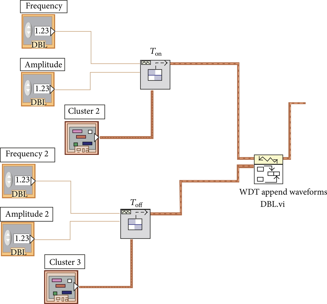
The “WDT Append Waveforms DBL.vi” (square wave synthesizer) in the LabVIEW program.
When it comes to the precise positioning of a stage, a position sensor is of vital importance. The accuracy of a position signal directly affects a control convergence result. Hence, there must be requirements of a position sensor, and considerations must be given to the position sensor. The precision of the RENISHAW optical scale used in the experiment can reach 0.1 μm. The optical scale features compactness, high resolution, quick responses, and ease of installation. The signal output from the optical scale is the clock voltage signal, and thus it has to be processed by the LabVIEW program and converted into a position signal before it is available for use. Signal analysis of the RENISHAW optical scale is shown in Figure 10(a). The optical scale signals we acquired from two experiments that represent a moving condition of the stage to left and to right are shown in Figures 10(b) and 10(c). Besides, we could find out that signal A leads by 90° phase difference over signal B by comparing two phases of Figure 10(b). On the other hand, signal A lags by 90° phase difference behind signal B by comparing two phases of Figure 10(c). As we can discover from Figures 10(b) and 10(c), the reasons which caused the cycle of these two signals to be unequal include that the moving speed of stage to left and to right is not the same, the piezoelectric actuator has a nonlinear effect, and the forward rotation and reverse rotation capability of actuator are unbalanced.

The signal diagrams of the optical scale: (a) a signal analysis diagram of two channels of the RENISHAW optical scale; (b) signal A leads by 90° phase difference over signal B; (c) signal A lags by 90° phase difference behind signal B.
6. Displacement Characteristic Measurement
In the experiment, the 4-9-9-14 piezoelectric actuator functions as a device for driving the stage, and the driving duration (T on time) is controlled in order to achieve stepping. Also, the driving frequency of the actuator is changed to vary the direction of the propulsion of the actuator. The driving voltage (for adjusting voltage amplitude) is varied to enable parameter adjustment required for adjustment of a displacement in the experiment.
6.1. Ton Time Adjustment
The driving frequency of a period is generated by LabVIEW program. In the experiment, the driving voltage of 2 Vp-p is fixed and then amplified tenfold by a power amplifier to generate the driving voltage of 20 Vp-p and serve as a fixed driving parameter of the actuator. It is necessary to change the driving frequency of the actuator, because the driving frequency of the actuator is of two types, namely, forward rotation frequency and reverse rotation frequency. The forward rotation frequency is 77.0 kHz and the reverse rotation frequency is 65.9 kHz. Afterward, a definition is given to the direction of the movement of the stage. Rightward movement of the stage is denoted by the plus sign “+.” Leftward movement of the stage is denoted by the minus sign “−.” Our research team conducts experiments on the upper stage and the lower stage, respectively, to explore the stepping propulsion of the stage by the piezoelectric actuator. Four types of experiments are conducted according to the parameter adjustment of the experiments: (1) the upper stage rightward stepping experiment, a driving voltage of 20 Vp-p, and T on time of 0.5 ms, 1 ms, 5 ms, and 10 ms; (2) the upper stage leftward stepping experiment, a driving voltage of 20 Vp-p and T on time of 0.5 ms, 1 ms, 5 ms and 10 ms; (3) the lower stage forward stepping experiment, a driving voltage of 20 Vp-p and T on time of 0.5 ms, 1 ms, 5 ms and 10 ms; (4) the lower stage backward stepping experiment, a driving voltage of 20 Vp-p, and T on time of 0.5 ms, 1 ms, 5 ms, and 10 ms.
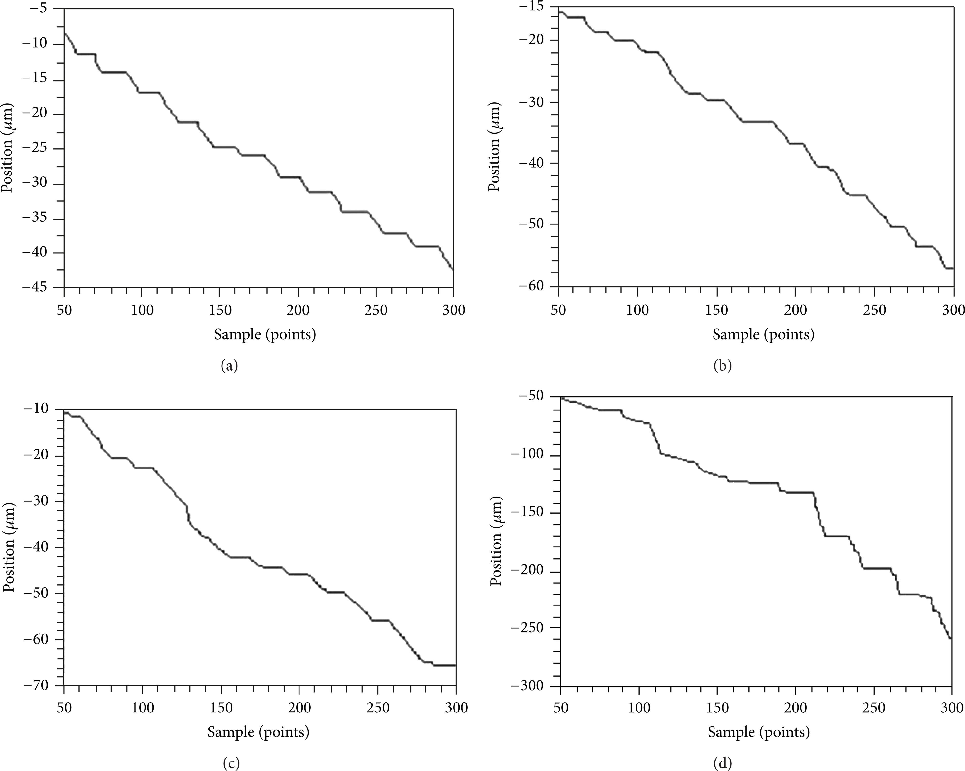
Results of the upper stage rightward stepping experiment and results of the upper stage leftward stepping experiment are shown in Table 1. Results of the lower stage forward stepping experiment and results of the lower stage backward stepping experiment are shown in Table 2. Figures 11 and 12 separately illustrate the rightward stepping experiment and the leftward stepping experiment of the upper stage. Figures 13 and 14 separately illustrate the forward stepping experiment and the backward stepping experiment of the lower stage. The diagrams show that a maximum of 300 samples are displayed.
A table of results of displacement measurement of the upper stage at the corrected T on time.

Unit (μm).
A table of results of displacement measurement of the lower stage at the corrected T on time.

Unit (μm).

A diagram of displacements in the upper stage rightward stepping experiment: (a) T on time of 0.5 ms; (b) T on time of 1 ms; (c) T on time of 5 ms; (d) T on time of 10 ms.
A diagram of displacements in the upper stage leftward stepping experiment: (a) T on time of 0.5 ms; (b) T on time of 1 ms; (c) T on time of 5 ms; (d) T on time of 10 ms.
A diagram of displacements in the lower stage forward stepping experiment: (a) T on time of 0.5 ms; (b) T on time of 1 ms; (c) T on time of 5 ms; (d) T on time of 10 ms.

A diagram of displacements in the lower stage backward stepping experiment: (a) T on time of 0.5 ms; (b) T on time of 1 ms; (c) T on time of 5 ms; (d) T on time of 10 ms.
The frequency of 65.9 kHz or 77.0 kHz is decided to be based on the displacement curve of the actuator under various frequencies (i.e., sweeping) by ANSYS simulation. The vector of displacement curve comes with 2 obvious peak values right on the frequencies of 65.9 kHz and 77.0 kHz. It means that, on these 2 frequencies, it will be featured with the more excellent driving effect (or displacement) [21].
6.2. Driving Voltage Adjustment
In the driving voltage parameter experiment, the adjusted parameter is the driving voltage magnitude of the actuator, and this situation occurs to the upper and lower stages because of nonuniform performance of the actuator in driving the stage to move leftward and rightward. To render stage movement capability uniform and thus facilitate stage control and positioning, our research team alters the driving voltage to equalize the leftward and rightward stepping performance. As a result, the upper stage leftward movement capability equals the upper stage rightward movement capability. Our research team increases the driving voltage to 25 Vp-p so as to boost the extension capability of the actuator, and thus the actuator has more energy for moving the stage; the same applies to the lower stage. However, considering that the lower stage bears the weight of the upper stage, our research team increases the driving voltages to 25 Vp-p and 30 Vp-p, respectively. Hence, this section describes experiments of stage stepping propulsion performed by the piezoelectric actuator on the upper stage and the lower stage, respectively. Four types of experiments of driving voltage parameter adjustment are as follows: (1) the upper stage rightward stepping experiment, a driving voltage of 20 Vp-p and T on time of 1 ms and 10 ms; (2) The upper stage leftward stepping experiment; a driving voltage of 25 Vp-p and T on time of 1 ms and 10 ms; (3) The lower stage forward stepping experiment; a driving voltage of 25 Vp-p, T on time of 1 ms and 10 ms; (4) The lower stage backward stepping experiment, a driving voltage of 30 Vp-p and T on time of 1 ms and 10 ms. Results of the upper stage rightward stepping experiment and results of the upper stage leftward stepping experiment are shown in Table 3.
A table of results of displacement measurement of the upper stage at the corrected driving voltage.
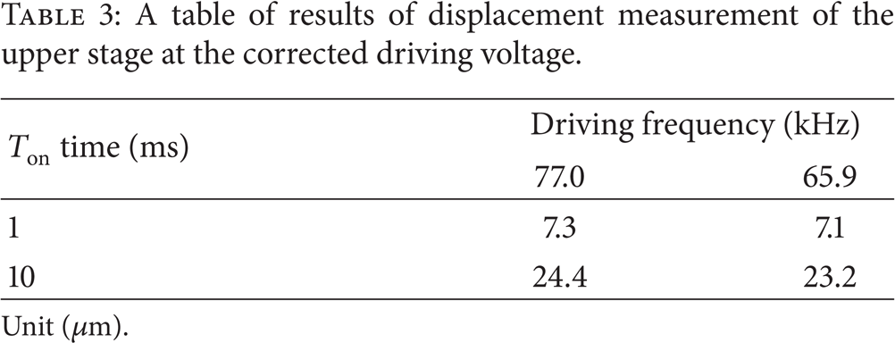
Unit (μm).
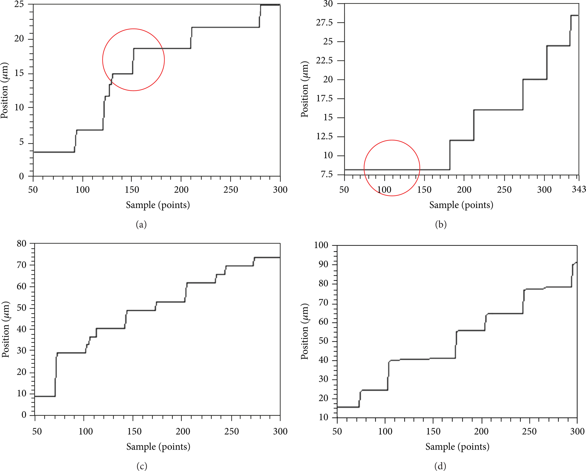
Results of the lower stage forward stepping experiment and results of the lower stage backward stepping experiment are shown in Table 4. Figures 15 and 16 separately illustrate the rightward stepping experiment and the leftward stepping experiment of the upper stage. Figures 17 and 18 separately illustrate the forward stepping experiment and the backward stepping experiment of the lower stage. The diagrams show that a maximum of 300 samples are displayed.
A table of results of displacement measurement of the lower stage at the corrected driving voltage.
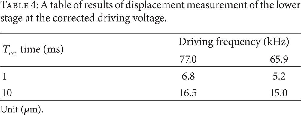
Unit (μm).

A diagram of displacements in the upper stage rightward stepping experiment: (a) driving voltage of 20 Vp-p and T on time of 1 ms; (b) driving voltage of 20 Vp-p and T on time of 10 ms.

A diagram of displacements in the upper stage leftward stepping experiment: (a) driving voltage of 25 Vp-p and T on time of 1 ms; (b) driving voltage of 25 Vp-p and T on time of 10 ms.

A diagram of displacements in the lower stage rightward stepping experiment: (a) driving voltage of 25 Vp-p and T on time of 1 ms; (b) driving voltage of 20 Vp-p and T on time of 10 ms.
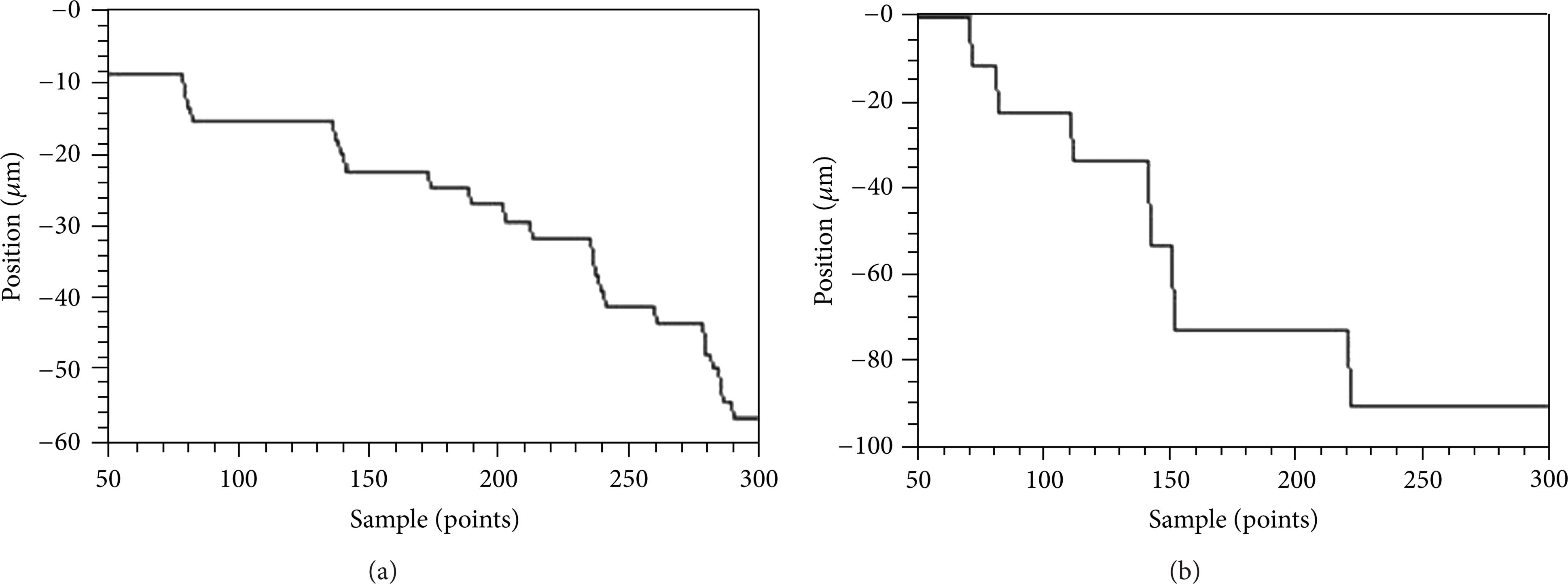
A diagram of displacements in the lower stage leftward stepping experiment: (a) driving voltage of 30 Vp-p and T on time of 1 ms; (b) driving voltage of 25 Vp-p and T on time of 10 ms.
7. Result and Discussion
As indicated by Table 1, given a constant driving voltage, the displacement of stage movement increases with T on time and decreases with T on time, and this phenomenon occurs to leftward or rightward movement of the upper stage and forward or backward movement of the lower stage. As indicated by the displacement-related data shown in Table 1, given a constant T on time, the displacement of rightward (or forward) movement of the upper (or the lower) stage is always larger than the displacement of leftward (or backward) movement of the upper (or the lower) stage. The result of the experiment proves that the actuator manifests stronger rightward (or forward) propulsion than leftward (or backward) propulsion. As indicated by Table 1, given a constant T on time, the upper stage always has a larger displacement than the lower stage, whether in leftward movement or rightward movement. Due to the mechanism whereby the lower stage underpins the upper stage, the lower stage has a heavy load. This leads to the inference that the displacement of leftward/rightward movement decreases as the load of the actuator in propulsion increases. Hence, the load of the actuator directly affects the difference in displacements.
As indicated by Tables 1 and 2, although leftward propulsion and rightward propulsion of the actuator are rendered uniform by correcting the driving voltage, it is impossible for the lower stage stepping capability to be corrected to such an extent so as to equal the upper stage stepping capability by correcting the driving voltage used in the lower stage. It is because the driving voltage is corrected to increase the potential difference and thereby increase the oscillation energy of the actuator. The 4-9-9-14 piezoelectric actuator used in the experiment is likely to crack in case of an excessive driving voltage and excessive input energy (with a driving voltage higher than 40 Vp-p), because of the small thickness (0.1 mm approximately) of a piezoelectric sheet used and the heat generated as a result of the stretching of the piezoelectric buzzer. If the voltage is increased continuously, the actuator may break down and become unusable. However, if the driving parameter of the upper stage is adjusted in a manner that the upper stage stepping capability approximates to the lower stage stepping capability, the upper stage stepping capability may diminish to the detriment of control.
Diagrams of stepping undertaken in the experiment indicate that waveforms of stage movement are of the following types. (1) The stage overstays: the stage will overstay, if the stage does not move by stepping continuously while being driven by the actuator, as shown in Figure 13(b). (2) In a single instance of movement, the stage moves by a distance longer than the average displacement: the actuator is capable of optimal actuation at 77 kHz, and thus the displacement in a single instance of movement is likely to exceed the average displacement, as shown in Figure 17(a).
Observation of a diagram of the upper stage stepping experiment as shown in Figure 11(a) and a diagram of the lower stage stepping experiment as shown in Figure 13(a) reveals that sliding seldom occurs to the lower stage stepping, not only because the lower stage carries a heavy load while the upper stage does not carry any load but also because it takes time for the system to respond, and thus the upper stage is more likely to undergo sliding. The upper stage stepping demonstrated by 300 samples shown in Figure 11(a) always has a larger displacement than the lower stage stepping demonstrated by 300 samples shown in Figure 13(a). The upper stage has no load while the lower stage has a heavy load; hence, the actuator has to accumulate propulsion energy in many more instances of propulsion in order to drive the lower stage to move.
In the experiment, if T on time is shorter than 0.5 ms, as shown in Figure 19(a), during the 0.5 ms time period, the actuator has approximately 30∼40 clocks generating energy (0.5 ms/(77.0 kHz)−1 ≈ 38.50 clocks, 0.5 ms/(65.9 kHz)−1 ≈ 32.95 clocks), and the energy accumulated by the actuator is almost insufficient to drive the stage, indicating that, when T on time is 0.5 ms, the stepping distance is 3 μm approximately; other possibilities include the surface roughness of the stage, errors in precision of assembly, characteristics of the V-shaped guide rail, and the limitation of the least movement. Hence, in the experiment, shorter T on time is not measured. In the experiment, if T on time is longer than 10 ms, as shown in Figure 19(b), during the 10 ms time period, the actuator has approximately 650∼800 clocks generating energy (10 ms/(77.0 kHz)−1 ≈ 777 clocks, 10 ms/(65.9 kHz)−1 ≈ 659 clocks), indicating that, when T on time is longer than 10 ms, the energy accumulated by the actuator may be too much, and the actuator can drive the stage efficiently, and in consequence the stage is likely to slide; if the stage slides too often, it will compromise precise positioning and control.

(a) A diagram of T on time shorter than 0.5 ms; (b) a diagram of T on time longer than 10 ms.
8. Conclusions
Most piezoelectric motors employ a stacked/multilayered piezoelectric material or an alternate polarization of electrodes of piezoelectric material. These piezoelectric materials are expensive, and thus commercially available piezoelectric motors are expensive, too. A piezoelectric motor developed by our research team is a 4-9-9-14 piezoelectric actuator that comprises an inexpensive piezoelectric buzzer. The purpose of the piezoelectric actuator is to position a stage in a mechanical system.
The movement of a stage is read and analyzed by means of LabVIEW operating in conjunction with an optical scale. Stage movement-related signals read by the optical scale are processed. With a human-machine interface of LabVIEW, the movement of the stage is depicted by a waveform chart to thereby facilitate the observation of the waveform chart and the understanding of propulsion of the stage by the actuator. A driving signal for driving the 4-9-9-14 piezoelectric actuator is generated by means of LabVIEW operating in conjunction with the NI PCI-6115 DAQ card. With the human-machine interface of LabVIEW, the signal sent is graphically displayed to facilitate the observation of the driving signal sent.
Given a constant driving voltage, the displacement of the stage increases with T on time, and the displacement of the stage decreases with T on time. The aforesaid phenomenon occurs to leftward or rightward movement of the upper stage and forward or backward movement of the lower stage. Given a constant T on time, the displacement of the stage in motion decreases with the driving voltage, and the displacement of the stage in motion increases with the driving voltage. As indicated by the result of the stepping experiment, a stepping distance increases with T on time; however, an analysis of the data gathered by the experiment reveals no linear correlation between the stepping distance and the T on time, and thus our research team attributes the aforesaid result of the stepping experiment to a hysteresis.
As indicated by the result of the stepping experiment, given a constant driving voltage and a constant T on time, the displacement of the stage moving rightward (at 77 kHz) is always larger than the displacement of the stage moving leftward (at 65.9 kHz), and the displacement of the lower stage moving forward is not consistent with the displacement of the lower stage moving backward. An experiment result relationship table verifies that, given the same driving signal but different propulsion directions, the 4-9-9-14 piezoelectric actuator is not consistent in its performance in the propulsion of the stage.
As indicated by the result of the stepping experiment, the driving voltage is corrected such that the actuator is consistent in its leftward propulsion and rightward propulsion and performs consistently whether applied to the upper stage or the lower stage. Although correcting the driving voltage enhances the consistency of the actuator in its leftward propulsion and rightward propulsion, the driving voltage is corrected so as to increase the potential difference and thereby increase oscillation energy of the actuator. If the driving voltage applied to the 4-9-9-14 piezoelectric actuator is too high, the energy thus supplied will be excessive (with the driving voltage exceeding 40 Vp-p) to thereby bring about a cracking-like phenomenon. If the driving voltage is adjusted and increased continuously, the actuator will be likely to get damaged and unusable.
During the experiment, given a T on time longer than 10 ms, the actuator is likely to accumulate excessive energy per unit area, and thus the actuator drives the stage excessively, thereby causing the stage to slide to the detriment of the subsequent positioning and controlling of the stage and thus the result of the experiment.
Conflict of Interests
The author declares that there is no conflict of interests regarding the publication of this paper.