Sage Journals: Discover world-class research

Abstract

This paper presents a digital image processing (DIP) based finite difference method (FDM) and makes the first attempt to apply the new method to the failure process of stratified rocks from Chinese Jinping underground carves. In the method, the two-dimensional (2D) inhomogeneity and mesostructures of rock materials are first identified with the DIP technique. And then the binarization image information is used to generate the finite difference grids. Finally, the failure process of stratified rock samples under uniaxial compression condition is simulated by using the FDM. In the DIP, an image segmentation algorithm based on seeded region growing (SRG) is proposed, instead of the traditional threshold value method. And with the new method, we can fully acquire the inhomogeneous distributions and mesostructures of stratified rocks. The simulated macroscopic mechanical behaviors are in good agreement with the laboratory experimental observation. Numerical results show that the proposed DIP based FDM is suitable for the failure analysis of stratified rocks because it can fully take into account the material heterogeneity, and the anisotropy of stratified rocks is also disposed to some extent.

1. Introduction

Stratified rocks are often met in rock engineering, and the full understanding of the mechanical behaviors of stratified rocks is useful and important to evaluate the stability of rock engineering built in the stratified rocks. Owing to the preferred fabric orientation and different rock materials, stratified rocks exhibit strong inherent anisotropy and heterogeneity. Over the past decades, scholars have mainly concentrated their attentions on the research to the anisotropy of stratified rocks. And the property of heterogeneity was almost not considered in the researches. For example, Salamon [1] studied the anisotropy of elastic moduli of a stratified rock mass. Jaeger [2] suggested the most popular discontinuous failure criteria named “the single plane of weakness theory” and Attewell and Sandford, McLamore and Gray, Duveau and Shao, Cazacu et al., and Huang [3 –7] extended this theory continuously. From the view of experiments, Tien et al. [8 –10] investigated the failure mechanism of synthetic stratified rock with varied orientations at different confining pressures. For ensuring underground excavations safety, Alejano et al. [11] employed multiapproach back-analysis including the numerical discrete element method to analyze roof bed deformation mechanics in stratified rock. In fact, the anisotropy of stratified rocks is strongly related to the mesostructures [12]. And the failure modes of stratified rocks are dependent on the internal mesostructures. Thus, it is significant to consider the property of heterogeneity of stratified rocks in the studies. And the key problem is how to accurately obtain the real heterogeneity and mesostructures.

DIP is the use of computer algorithms to perform image processing on digital images [13]. The DIP technique provides an innovative mean to acquire the real heterogeneity and mesostructures of inhomogeneous materials. With the fast computers and signal processors available, the DIP has been widely used in a range of engineering topics in recent years [14, 15]. Yue et al. [16, 17] carried out quantitative investigations of the orientations, distributions, and shapes of aggregates in asphalt concrete using a DIP procedure. Obaidat et al. [18] further examined the percentage of voids in mineral aggregates of bituminous mixtures. Mora et al. [19] and Kwan et al. [20] investigated the particle shape characteristics of coarse aggregates using the DIP based methods. Lawler et al. [21] employed DIP method to observe cracks appearing in concrete. And the present research is mainly focused on the application of the DIP, combined with certain numerical methods, to study the mechanical property of inhomogeneous materials. Yue et al. [22] developed a DIP based finite element method and studied the effect of the shape of aggregate particles and their spatial distribution on the mechanics of mixture in asphalt concrete. Du et al. [23] adopted finite element model to simulate the cracks location on the basis of reconstruction of the internal structures for concrete composites using the DIP based method. Using DIP method based on X-ray computed tomography, Zelelew and Papagiannakis [24] proposed a methodology for simulating the creep behavior of asphalt concretes by the discrete element method. Chen et al. [25] presented a digital image based finite difference approach to analyze the failure process of rock samples by taking into account the actual 3D heterogeneity. It is worth noting that, in the DIP method, the traditional threshold segmentation algorithm is usually employed. The threshold segmentation algorithm assumes that all pixels whose value (gray level, color value, or others) lies within a certain range belong to one class; thus it neglects all of the spatial information of the image and does not deal well with noise or blurring at boundaries. To the best of the authors’ knowledge, the application of DIP in solving the stratified rock failure has not, as yet, been reported in literatures.

In this paper, the DIP based FDM is developed to analyze the stratified rock failure. In the proposed method, the 2D heterogeneity and mesostructures of stratified rock materials are first identified using the DIP technique, the finite difference grids are then generated according to the transforming information of binary images, and finally the failure process of stratified rock samples from Chinese Jinping underground carves under uniaxial compression condition is simulated with the FDM and the DIP based grids. In order to fully consider the spatial information of the image, an image segmentation algorithm based on SRG is proposed to detect the different individual materials and components automatically.

A brief outline of the rest of this paper is as follows. Section 2 presents the identification of heterogeneity and mesostructures of stratified rocks by using the DIP in detail. Generation of finite difference grids is then described in Section 3. In Section 4, numerical results obtained using the method proposed are presented and compared with the laboratory experimental observation. Finally, some conclusions and remarks are provided in Section 5.

2. Identification of Heterogeneity and Mesostructures

In this section, the big picture of the DIP technique is briefly introduced. Then, the pretreatments and the segmentation algorithm based on SRG are adopted to dispose the original image of sample surface.

2.1. DIP Technique

In general, a planar image can be defined as a 2D function, where x and y are spatial coordinates, and the amplitude of reflecting the brightness at point (x, y) is called the gray level of the image at the point. In other words, an image may be continuous with respect to the x and y coordinates and also in amplitude. When x, y, and the gray level are finite and discrete quantities, the digital image is presented. In fact, the digital image consists of a rectangular array of image elements named pixels. Each pixel is the intersection area of any horizontal scanning line with the vertical scanning line. All of these lines have an equal width h. As a result, the digital image can be expressed as a discrete function in the i and j Cartesian coordinate system as follows:

f (i, j) = [\begin{bmatrix} f (1,1) & f (1,2) & \dots & f (1, m) \\ f (2,1) & f (2,2) & \dots & f (2, m) \\ ⋮ & ⋮ & ⋮ \\ f (n, 1) & f (n, 2) & \dots & f (n, m) \end{bmatrix}],

(1)

where i changes from 1 to n and j changes from 1 to m.

Furthermore, the DIP can apply various mathematical algorithms by means of computers to extract significant information from the digital image. This information may be characteristics of cracks on a material surface, the mesostructures of inhomogeneous soils and rocks, other man-made geomaterials, and so on. For rock materials, digital images can exactly depict and preserve the details of inhomogeneity and the relative position of mesostructures. And DIP technique is the ideal method for obtaining mesostructural information of rock materials surfaces from digital images.

Figure 1 shows the mostly used 256 gray images of a typical stratified rock sample surface, foliated metamorphic rock sample Y02-2 surface from Jinping underground carves. And the example of discrete function f(i, j) for the digital image is also included where the center of the i and j coordinate system is located at the top left corner of the image. According to research requirements, pixels are usually used to control the accuracy of the digital image as illustrated in Figures 1(a) and 1(b). For the original image shown in Figure 1(b), the numbers of the scanning lines along the i-axis and the j-axis are 100 and 100, respectively. The actual size of the sample is 50 mm × 50 mm. So, the scanning line is 0.5 mm wide and pixel size is 0.5 mm × 0.5 mm.

Figure 1:

An example of original discrete function f(i, j) of digital image sample Y02-2: (a) original image of 50 × 50 pixels; (b) original image of 100 × 100 pixels; (c) some part of original image (local i and j coordinate system); (d) matrix of discrete function f(i, j) (local i and j coordinate system).

2.2. Pretreatments of Digital Image

Because the process of converting actual sample into digital images is very complicated and easily affected by external environment (e.g., asymmetric illumination and electrical and mechanical noise), the digital image quality is usually not good enough to acquire well-defined material mesostructures. Thus, image pretreatments, such as image contrast enhancement and image noise elimination methods based on direct manipulation of pixels, are necessary to obtain a more reasonable result for the material mesostructures.

For the image contrast enhancement, it can help to gain material mesostructures due to its improvement of the contrast between different inner materials. The commonly used image enhancement method is known as the histogram equalization transformation. The histogram of a digital image is used to display the distribution of gray values in the image. It is a discrete function to show, for each gray level, the number of pixels that have that gray level. Generally, it is useful to work with normalized histograms, obtained simply by dividing all the numbers above by total amount of pixels in the image. And histogram equalization adopts some transformations shown in [13] to deal with normalized histograms and acquires a new histogram which ensures that all gray levels displayed have approximately equal probability to represent, although by this way the histogram of processed image will not be uniform as before; in other words, the result of the gray level equalization process can provide an image with increased dynamic range, which tends to have higher contrast.

Because image noise can be generated in many ways, noise elimination methods are various in response. In order to reduce noise influence on acquiring mesostructures, the median filter, which can protect the edges of different parts, is adopted here. Median filter, as an applicable method, is a nonlinear function that is carried out on the pixels of a neighborhood and whose result constitutes the response of the operation at the center pixel of the neighborhood. In general, the median filter operates with a defined 3-by-3 neighborhood by sliding the center point of it through the image. And the pixel value in the image is replaced by median value of its neighboring pixels. For the pixels on the image boundaries, the median filter performs the transformation by padding the image with zeros [26].

Using the original image shown in Figure 1(b) as an example, Figure 2 shows the pretreatment results. Compared with original image, the new image achieves enhancements among the different inner materials and preserves more details of mesoinformation.

Figure 2:

The image pretreatment results of sample Y02-2: (a) histogram equalization processed image; (b) median filter processed image.

2.3. Image Segmentation Technique Based on SRG

In this subsection, image segmentation algorithm based on SRG is presented to acquire the actual mesostructures of stratified rock materials. Using the above sample Y02-2 surface image (100 × 100) as an example, the algorithm is employed to partition the image. And a binary image is outputted as mesostructures of the sample surface.

2.3.1. Image Segmentation and SRG

Image segmentation refers to subdividing an image into its constituent regions or objects. The level to which the subdivision is carried depends on the problem itself. Segmentation algorithms for gray-scale images generally are based on two basic properties of image gray value: discontinuity and similarity. SRG and traditional threshold algorithm are both on the basis of similarity property. However, due to the property of rock materials, the gray level of each material is not an exact value but an interval. So it is common that some overlap of gray level interval among rock materials is presented. This case may lead to inaccurate segmentation by using traditional threshold algorithm. Because the threshold algorithm assumes that all pixels whose value (gray level, color value, or others) lies within a certain range belong to one class, thus, in this circumstance, SRG algorithm which can fully consider the spatial information of materials in the image is adopted in the research.

In fact, SRG is a procedure that groups pixels or subregions into larger regions based on predefined criteria for growth. The basic approach is to start with a number of seeds which have been classified into n sets, say, A₁, A₂,…, A_n, and form these growing regions by appending to each A_i those neighboring pixels that have predefined properties similar to the seed. Selecting a set of one or more starting points often can be decided by the nature of the problem. And the choice of similarity criteria is critical for even moderate success in region growing [27, 28]. Generally, three types of expression are given: criterion based on gray value difference, criterion based on gray value distribution, and criterion based on region shape. When no pixels satisfy the criteria for inclusion in that region, growing a region should stop.

2.3.2. Implement of SRG

In this paper, the purpose of segmentation is to partition the image (Figure 1(b)) into two regions, that is, greenschist region (growing region) which is darker in the image and marble region (ungrowing region) which is brighter. Firstly, in order to acquire better segmentation results, nine seed points, namely, the initial state of the sets A₁, A₂,…, A₉ consisting of single points, respectively, is manually chosen from Figure 2(b). Their coordinates are shown in Table 1. Then, the indicator matrix used to record the growing process is formed. It has the same size with the rectangle array of Figure 2(b) and all its initial elements are filled by label “0.” Afterward, the corresponding elements in the indicator matrix to seeds are changed to the label “1.” For the set A_i, each step loop of the algorithm hopes to add one pixel to it. The state of A_i after m steps will be considered as follows. Let T be the set of growing pixels which border ungrowing region:

T = {x \in ⋃_{i = 1}^{n} A_{i} ∣ N (x) \cap C_{R} ⋃_{i = 1}^{n} A_{i} \neq ϕ},

(2)

where N(x) is the immediate neighbors of the pixel x and R represents entire region of the digital image. In other words, T is a data structure termed queue of border pixels (QBP). It is just an array of objects. When considering a new pixel, at the beginning of each step of SRG, we take that one at the beginning of the array. For example, in the m + 1 step, pixel x is taken from T. And for the segmentation process to be presented, the immediate neighbors which are 8-connected to the pixel x are used. δ[N_i(x)] is defined to be a measure of how different the pixel N_i(x) is from the growing region it adjoins, where i belongs to {1, 2,…, 8}. The simplest definition for δ[N_i(x)] is

δ [N_{i} (x)] = | f [N_{i} (x)] - f (y) |,

(3)

where f[N_i(x)] and f(y) are the gray value of the pixel N_i(x) and seed point y which belongs to the growing region, respectively.

Table 1:

The coordinates and response thresholds of individual seeds.

Number of pixel points	Coordinates of pixel points	Threshold of pixel points

1	(92, 8)	37
2	(89, 36)	25
3	(53, 38)	4
4	(42, 44)	7
5	(34, 37)	10
6	(7, 39)	10
7	(54, 71)	20
8	(28, 87)	22
9	(37, 59)	15

The similarity criterion based on gray value difference is given as follows:

P (R_{j}) = {\begin{cases} TRUE, & δ [N_{i} (x)] \leq Δ, \\ FALSE, & otherwise, \end{cases}

(4)

where R_j represents the subregion of entire image region R and has the property that ⋃_{j = 1}ⁿ R_{j = R}; P is a predicate.

Equation (4) notes that, for the pixel N_i(x), if the gray value difference to the growing region it adjoins is in the predefined range of Δ, the pixel N_i(x) will belong to the region. That is, the corresponding label in the indicator matrix to the pixel N_i(x) will be changed to the label of the pixel x. Meanwhile, the pixel N_i(x) is put in the end of data structure T. And the pixel x is deleted in the data structure T. This completes step m + 1. The process is repeated until no pixels are in the data structure T. The flow chart of the algorithm is shown in Figure 3. For threshold Δ, a trial-and-error method can be used to adjust it so that the best results are obtained. And the thresholds that correspond to the nine individual seeds are shown in Table 1.

Figure 3:

The flow chart of the SRG algorithm for individual seed.

After segmentation, some holes and gaps may still exist in images. The morphological closing and filling method shown in [26] are used to get rid of them. Figure 4 reflects the whole process of segmentation of the sample Y02-2 surface.

Figure 4:

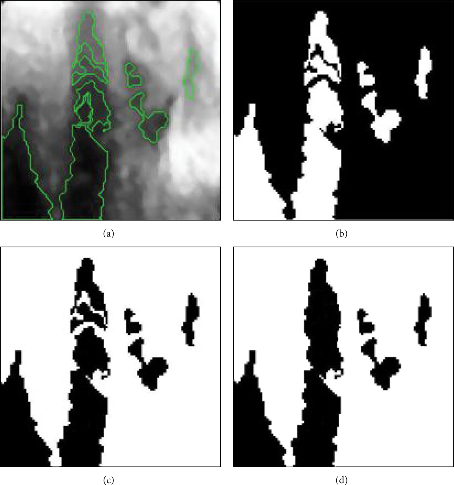
The whole process of segmentation of the sample Y02-2 surface: (a) the outline formed by SRG; (b) the binary image after segmentation; (c) the negative image of (b); (d) the binary image after morphological mend.

3. Generation of Finite Difference Grids

In order to carry out the numerical analysis, finite difference grids must be generated according to the material distribution and geometry shown in the binary image of final output in the process of segmentation. However, the finite difference grids cannot be generated directly from the binary images. The binarization information is required to be transformed. As mentioned above, binary images are special discrete rectangular arrays and their gray values of pixels are either 0 or 1. Therefore, the image can be considered as equivalent grids. Consider the binary image (Figure 5(a)) transforming from Figure 1(c) as an example; basic grids are established by dealing with pixels in the image as elements and pixel angular points as nodes shown in Figure 5(b). At the same time, the corresponding array of pixel values to binary image, the gray value 1 used to represent bright marble pixels and the gray value 0 used to represent dark greenschist pixels, can provide exact distribution of the two rock materials, as shown in Figure 5(c). Thus, combining the basic grids and distribution information of pixel values, finite difference grids considering actual heterogeneity and mesostructures are generated, as shown in Figure 5(d). And the finite difference grids corresponding to digital image of sample Y02-2 are shown in Figure 6. The size of grids is 50 mm × 50 mm and the scale of rectangle element is 0.5 mm × 0.5 mm.

Figure 5:

An example of finite difference grids generation: (a) transforming from some part of original image; (b) basic grids; (c) matrix of discrete function f(i, j); (d) finite difference grids (local i and j coordinate system).

Figure 6:

Finite difference grids containing real mesostructures.

The precision of this grids generation method depends on pixels, while it is not complicated to implement this method. By transforming binarization image information, the actual mesostructures preserved in pixels of image, especially the shapes of rock material interfaces, are shown in this method. So, finite difference grids generated by the method keep highly consistent with real mesostructures and inhomogeneity.

4. Numerical Simulation

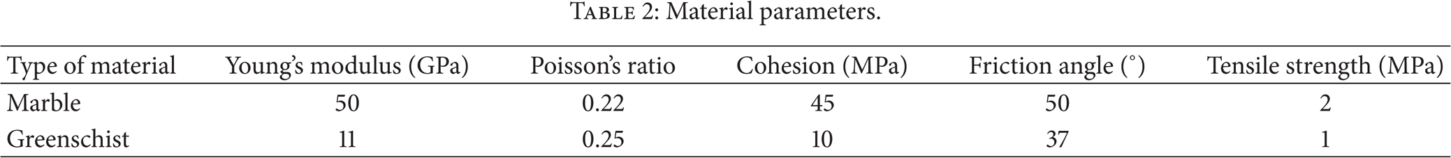
In this section, an explicit finite difference scheme will be employed to simulate fracture propagation of foliated metamorphic rock sample Y02-2 from Chinese Jinping underground carves under uniaxial compression loadings, as shown in Figure 7. The commercial software FLAC (Fast Lagrangian Analysis of Continua) is used for finite difference analyses. In the analysis, the mesolevel calculation grids based on the actual inhomogeneity and mesostructures of stratified rocks are used; the Mohr-Coulomb failure criterion is adopted. Fracture propagation is considered by the progressive tension and shear failure. Table 2 shows the material parameters referring to [7, 29, 30].

Table 2:

Material parameters.

Type of material	Young's modulus (GPa)	Poisson's ratio	Cohesion (MPa)	Friction angle (°)	Tensile strength (MPa)

Marble	50	0.22	45	50	2
Greenschist	11	0.25	10	37	1

Figure 7:

Schematic diagram of the sample: (a) vertical loading; (b) horizontal loading.

4.1. Vertical Loading

Figure 8 depicts the axial force-displacement curve of the sample in vertical loading condition obtained by the developed method. It is observed that there are three distinct mechanical response stages in the force-displacement curve. In the first stage, before the applied load reached the peak (approximately 2.25 kN), there is a linear relationship between the load increment and displacement increment. This stage shows the elastic feature. In the second stage, the applied load rapidly drops, while the vertical displacement increases. This stage shows the brittle feature. In the third stage, the displacement continues to increase as the load remains unchanged. This stage shows the perfect plastic feature.

Figure 8:

The axial force-displacement curve under vertical loading condition.

Figure 9 shows the progressive failure processes, and they correspond to the five points of the axial force-displacement curve, such as points (a) to (e). It is observed from the results that (1) at point (a) of the force-displacement curve tension failure first occurs, and most failure domains locate at the right thin greenschist layer; few failure domains are from the middle and left major greenschist layers, as shown in Figure 9(a); (2) increasing the applied load to point (b), the tension failure domains slowly increase, and the shear failure appears at right thin and left major greenschist layers; (3) as the fractures grow and coalesce, a large amount of shear failure domains is formed in the thin and major greenschist layers along their long-axial directions, and at last the sample is destroyed because most failure domains link up few tension failure domains; (4) the final fracture mode is quite different from the traditional “X” failure mode of homogenous materials under vertical loading, and the final fracture mode matches well with the laboratory experimental observation as shown in Figure 10.

Figure 9:

Simulated fracture process of the sample under vertical loading condition (red: tension failure; blue: shear failure): (a) the failure domains corresponding to point (a) of force-displacement curve; (b) the failure domains corresponding to point (b) of force-displacement curve; (c) the failure domains corresponding to point (c) of force-displacement curve; (d) the failure domains corresponding to point (d) of force-displacement curve; (e) the failure domains corresponding to point (e) of force-displacement curve.

Figure 10:

Final result observation of the sample in laboratory uniaxial compression experiment.

4.2. Horizontal Loading

Figure 11 shows the axial force-displacement curve of the sample under horizontal loading condition obtained by the developed method. The elastic-brittle-plastic property of sample can be displayed too. Due to the influence of inhomogeneity and mesostructures, the shape of the force-displacement curve under horizontal loading is different from that under vertical loading to some extent.

Figure 11:

The axial force-displacement curve in horizontal loading condition.

Figure 12 presents the progressive failure processes, and they correspond to the five points of the axial force-displacement curve, such as points (a) to (e), as shown in Figure 11. It is observed from the results that, (1) at point (a) of the force-displacement curve, tension failure first occurs, and most failure domains locate at the middle major greenschist layer; (2) increasing the applied load to point (b), the tension failure domains slowly increase, and the shear failure appears at the middle major greenschist layers, and the failure domain has some angle with short-axial direction of middle major greenschist layers; meanwhile, shear failure appears to some degrees at right thin and left major greenschist layers; (3) as the fractures grow and coalescence, a large amount of tension failure domains is formed, and the development trend is roughly parallel to loading direction.

Figure 12:

Simulated fracture process of the sample under horizontal loading condition (red: tension failure; blue: shear failure): (a) the failure domains corresponding to point (a) of force-displacement curve; (b) the failure domains corresponding to point (b) of force-displacement curve; (c) the failure domains corresponding to point (c) of force-displacement curve; (d) the failure domains corresponding to point (d) of force-displacement curve; (e) the failure domains corresponding to point (e) of force-displacement curve.

From Figures 9 and 12, it is found that tension failure first occurs and a large amount of shear failure domains yields the final destruction for vertical and horizontal loadings.

However, there are some differences in details; for example, the shear failure is along the long-axial direction for the vertical loading and approximately along the short-axial direction of major greenschist layer for the horizontal loading. It may be the anisotropy of rock mass.

5. Conclusions

In this paper, a DIP based FDM is developed to investigate the failure process of stratified rocks. In the method, the 2D inhomogeneity and mesostructures of rock materials are identified with the DIP technique, the binarization image information is then used to generate the finite difference grids, and the failure process of stratified rock samples under uniaxial compression condition is simulated with the FDM. The simulated macroscopic mechanical behaviors are in a good agreement with the laboratory experimental observation. Several key pointes may be drawn from the present study as follows.

The inhomogeneous distributions and mesostructures of foliated metamorphic rocks can be well obtained with the image segmentation algorithm based on SRG.

The inhomogeneity and mesostructures, the anisotropy, and the loading directions have significant effects on the fracture propagation process of stratified rocks.

The DIP based FDM is suitable for the failure analysis of stratified rocks because it can fully take into account the material heterogeneity, and the anisotropy of stratified rocks is also disposed to some extent.

Conflict of Interests

The authors declare that there is no conflict of interests regarding the publication of this paper.

Footnotes

Acknowledgment

The work described in this paper was supported by the National Natural Science Foundation of China (nos. 50978083, 51278169, and 11002048).

References

Salamon

M. D. G.

, “Elastic moduli of a stratified rock mass,” International Journal of Rock Mechanics and Mining Sciences and, vol. 5, no. 6, pp. 519–527, 1968.

Jaeger

J. C.

, “Shear failure of anistropic rocks,” Geological Magazine, vol. 97, no. 1, pp. 65–72, 1960.

Attewell

P. B.

and Sandford

M. R.

, “Intrinsic shear strength of a brittle, anisotropic rock–I: experimental and mechanical interpretation,” International Journal of Rock Mechanics and Mining Sciences & Geomechanics Abstracts, vol. 11, no. 11, pp. 423–430, 1974.

McLamore

and Gray

K. E.

, “The mechanical behavior of anisotropic sedimentary rocks,” Journal of Engineering for Industry, vol. 89, pp. 62–73, 1967.

Duveau

and Shao

J. F.

, “A modified single plane of weakness theory for the failure of highly stratified rocks,” International Journal of Rock Mechanics and Mining Sciences, vol. 35, no. 6, pp. 807–813, 1998.

Cazacu

Cristescu

N. D.

, and Shao

J. F.

, “A new failure criterion for transversely isotropic rocks,” International Journal of Rock Mechanics and Mining Sciences & Geomechanics Abstracts, vol. 35, no. 4–5, paper 130, 1996.

Huang

S. H. L.

, Study of mechanical model of brittle rock under high stress condition and its engineering applications [Ph.D. thesis], Graduate University, Chinese Academy of Sciences, Wuhan, China, 2008, (Chinese).

Tien

Y. M.

and Tsao

P. F.

, “Preparation and mechanical properties of artificial transversely isotropic rock,” International Journal of Rock Mechanics and Mining Sciences, vol. 37, no. 6, pp. 1001–1012, 2000.

Tien

Y. M.

and Kuo

M. C.

, “A failure criterion for transversely isotropic rocks,” International Journal of Rock Mechanics and Mining Sciences, vol. 38, no. 3, pp. 399–412, 2001.

10.

Tien

Y. M.

Kuo

M. C.

, and Juang

C. H.

, “An experimental investigation of the failure mechanism of simulated transversely isotropic rocks,” International Journal of Rock Mechanics and Mining Sciences, vol. 43, no. 8, pp. 1163–1181, 2006.

11.

Alejano

L. R.

Taboada

García-Bastante

, and Rodriguez

, “Multi-approach back-analysis of a roof bed collapse in a mining room excavated in stratified rock,” International Journal of Rock Mechanics and Mining Sciences, vol. 45, no. 6, pp. 899–913, 2008.

12.

Brady

B. H. G.

and Brown

E. T.

, Rock Mechanics for Underground Mining, Springer, 3rd edition, 2004.

13.

Gonzalez

R. C.

and Woods

R. E.

, Digital Image Processing, Prentice-Hall, Upper Saddle River, NJ, USA, 2nd edition, 2002.

14.

Frost

J. D.

and Wright

J. R.

, Digital Image Processing: Techniques and Applications in Civil Engineering, EF/NSF Conference, A.S.C.E., Hawaii, USA, 1993.

15.

Frost

J. D.

and McNeil

, Eds., Imaging Technologies—Techniques and Applications in Civil Engineering: Proceedings, Second International Conference on Imaging Technologies; May 25–30, 1997, Davos, Switzerland, A.S.C.E., 1998.

16.

Yue

Z. Q.

and Morin

, “Digital image processing for aggregate orientation in asphalt concrete mixtures,” Canadian Journal of Civil Engineering, vol. 23, no. 2, pp. 480–489, 1996.

17.

Yue

Z. Q.

Bekking

, and Morin

, “Application of digital image processing to quantitative study of asphalt concrete microstructure,” in Transportation Research Record 1492, pp. 53–60, Transportation Research Board, National Research Council, Washington, DC, USA, 1995.

18.

Obaidat

M. T.

Al-Masaeid

H. R.

Gharaybeh

, and Khedaywi

T. S.

, “An innovative digital image analysis approach to quantify the percentage of voids in mineral aggregates of bituminous mixtures,” Canadian Journal of Civil Engineering, vol. 25, no. 6, pp. 1041–1049, 1998.

19.

Mora

C. F.

Kwan

A. K. H.

, and Chan

H. C.

, “Particle size distribution analysis of coarse aggregate using digital image processing,” Cement and Concrete Research, vol. 28, no. 6, pp. 921–932, 1998.

20.

Kwan

A. K. H.

Mora

C. F.

, and Chan

H. C.

, “Particle shape analysis of coarse aggregate using digital image processing,” Cement and Concrete Research, vol. 29, no. 9, pp. 1403–1410, 1999.

21.

Lawler

J. S.

Keane

D. T.

, and Shah

S. P.

, “Measuring three-dimensional damage in concrete under compression,” ACI Materials Journal, vol. 98, no. 6, pp. 465–475, 2001.

22.

Yue

Z. Q.

Chen

, and Tham

L. G.

, “Finite element modeling of geomaterials using digital image processing,” Computers and Geotechnics, vol. 30, no. 5, pp. 375–397, 2003.

23.

Jiang

Qin

, and Lei

, “Reconstruction of internal structures and numerical simulation for concrete composites at mesoscale,” Computers and Concrete, vol. 10, no. 2, pp. 135–147, 2012.

24.

Zelelew

H. M.

and Papagiannakis

A. T.

, “Micromechanical modeling of asphalt concrete uniaxial creep using the discrete element method,” Road Materials and Pavement Design, vol. 11, no. 3, pp. 613–632, 2010.

25.

Chen

Yue

Z. Q.

, and Tham

L. G.

, “Digital image based approach for three-dimensional mechanical analysis of heterogeneous rocks,” Rock Mechanics and Rock Engineering, vol. 40, no. 2, pp. 145–168, 2007.

26.

Gonzales

R. C.

and Woods

R. E.

, Digital Image Processing Using Matlab, Prentice-Hall, Upper Saddle River, NJ, USA, 2nd edition, 2004.

27.

Pavlidis

and Liow

, “Integrating region growing and edge detection,” IEEE Transactions on Pattern Analysis and Machine Intelligence, vol. 12, no. 3, pp. 225–233, 1990.

28.

Adams

and Bischof

, “Seeded region growing,” IEEE Transactions on Pattern Analysis and Machine Intelligence, vol. 16, no. 6, pp. 641–647, 1994.

29.

Deng

R. G.

and Zhang

, “On the microstructure and mechanical properties of greenschist in the dam site of Jinping Hydropower Station,” Journal of Chengdu University of Technology, vol. 28, no. 1, pp. 93–97, 2001 (Chinese).

30.

Chengdu Hydroelectric Investion and Design Institute and China Hydropower Engineering Consulting Group Co, “The research report of check of dam site of Jinping I Hydropower Station at Yalong River (3): engineering geology condition,” Chengdu Hydroelectric Investigation and Design Institute, China Hydropower Engineering Consulting Group Co., Chengdu, China, 2003 (Chinese).

Mesoscopic Numerical Simulation of Stratified Rock Failure Using Digital Image Processing

Abstract

1. Introduction

2. Identification of Heterogeneity and Mesostructures

2.1. DIP Technique

2.2. Pretreatments of Digital Image

2.3. Image Segmentation Technique Based on SRG

2.3.1. Image Segmentation and SRG

2.3.2. Implement of SRG

3. Generation of Finite Difference Grids

4. Numerical Simulation

4.1. Vertical Loading

4.2. Horizontal Loading

5. Conclusions

Conflict of Interests

Footnotes

Acknowledgment

References