Sage Journals: Discover world-class research

Abstract

During the machining of complicated curves and surfaces, the massive microsegments are generated. The microsegments are inputted into numerical control system (CNC) to process the velocity planning and high-velocity interpolation. This whole procedure is the core algorithm of CNC. During the procedure of velocity planning, the look-ahead iterative calculation is used for several specified future microsegments and the calculation quantity is very large. Additionally, the CNC is a typical hard real-time system. Every interpolation step must be finished in specified interpolation period, so the high calculating ability of CPU is needed. The concept of GPU is quite different from the traditional CPU. It has a very strong parallel computing ability. In this project, the GPU technology is introduced into CNC algorithm. The parallel structure model is constructed by CUDA, and a discrete planning unit look-ahead velocity control strategy is proposed. The GPU parallel computing mechanism of massive microsegments is discussed and, based on the research, a high-performance velocity planning algorithm is presented. This research result can highly raise the velocity planning and interpolation efficiency. This brand new solution can help improve the performance of CNC system dramatically.

1. Introduction

High-velocity and high-accuracy complicated curve and surface processing is the main criterion of the numerical control technology. By CAD/CAM software, we use the simple line segment to approach the theoretical contour within the allowed trajectory error range. Then the numerical microsegments are generated and fed to interpolation module. There are three key problems for microsegment interpolation:

in order to satisfy the machining accuracy of complicated curve and surface, the number of microsegment is very large always;

the frequent acceleration/deceleration on each microsegment will increase the load of the motor. Additionally, the motion noise is generated and the control accuracy is lowered. Finally, the service life of motor is shortened. Therefore, the velocity planning for the whole set of microsegments is required and the optimal acceleration/deceleration characteristics can be achieved;

since the microsegment is very tiny, there is not enough length to finish the complete acceleration/deceleration procedure. The instruction velocity cannot be reached. The efficiency is lowered.

Therefore, to find an ideal curve and surface microsegment velocity planning and interpolation algorithm is the core problem of high-velocity and high-accuracy CNC.

The traditional microsegment velocity planning strategy based on CPU introduces the concept of “velocity look-ahead.” The look-ahead procedure is as follows: when computing the optimal interpolation velocity of the current microsegment, we will consider the geometric characteristics, transfer characteristics, and dynamic characteristics of several future microsegments [1 –3]. Based on velocity look-ahead strategy, we can avoid the unnecessary acceleration/deceleration during the whole interpolation procedure.

Nowadays, experts have done a lot of work on the look-ahead algorithm. The look-ahead strategy has already been used in many ways such as in NURBS interpolation [1, 4 –6] and Bézier curve interpolation [2, 3]. In [7 –9], the calculation equation of angle between two consecutive line blocks is given out but is not related to the angle of arc blocks. In [10], a new interpolation method is proposed; this algorithm realized the continuous computation of path segments, but, in the transferring point of consecutive segments, the path accuracy is decreased. In [11 –14], the linear acc/dec algorithm is introduced into the velocity look-ahead processing and constructs the path segment feedrate connecting model. Because of the shortage of linear acc/dec algorithm, the acceleration sudden change exists. The profile of velocity is not smooth and so it is not suitable for high-speed machining.

From all above research works, we can see that the velocity look-ahead computing procedure in CPU is a sequential computation procedure for every microsegment in each interpolation period. This sequential mode means that while even improving the CPU computation ability, for complicated curve or surface, the computation must comply with the specified order. With the increase of look-ahead segment number, the computation increases in exponential way. This serial arithmetic mode limits the algorithm efficiency. Therefore, the parallel mechanism research work for look-ahead algorithm is becoming a feasible scheme to improve the efficiency of the algorithm.

GPU (graphic processing unit) uses a large number of execution units. These units can be loaded using parallel processing easily. With the development of the GPU technology, it is used in many other general computation fields except graphical application [15 –17]. In [18], an algorithm of computing Bézier surface is presented. The triangular mesh is searched and extracted in real-time way by GPU. In [19], the parallel algorithm of GPU is used in computing NURBS curve and surface. From above we can find more and more researchers who already used the GPU in general purpose GPU field (GPGPU) other than graphical purpose. Therefore, the GPU parallel computation technology is introduced into control field as a new meaningful attempt.

The rest of the paper is organized as follows. In Section 2, we propose our whole scheme of parallel velocity planning algorithm with GPU. Interpolation geometry elements linking vector angle model is proposed in Section 3. In Sections 4 –7, the details of our parallel algorithm are proposed. In Section 8, the experiment result based on the new algorithm is presented. The conclusion and the future work are given in Section 9.

2. Whole Scheme of Parallel Velocity Planning Algorithm with GPU

In order to describe the whole trajectory curvature changes, we can focus on two ideas. First, the trajectory is regarded as a whole one, and the trajectory endpoints of the whole microsegments are regarded as the known points for fitting or interpolation. In other words, the analytical description is found for the microsegment trajectory. However, the disadvantage of this method is very obvious. The numerous microsegments make the fitting trajectory very complicated, so it is almost impossible to find a suitable curve to describe the whole trajectory easily.

Because of this disadvantage, this paper presents a new strategy. In order to develop the powerful parallel computer ability of GPU, in this paper we introduce a new concept named interpolation trajectory discretization. It means dividing the trajectory into several parts and then using special algorithm to describe the curvature and the maximum interpolation velocity of each part by powerful GPU parallel computing ability. Based on these results, we then deal with the overall velocity of whole trajectory. By this way, we can improve the efficiency of the algorithm, reduce the processing time, and improve the real-time ability of the system.

In this paper, a small part of the whole trajectory is called a planning unit; the specific meaning and the length determination of the planning unit will be presented in this paper. In the following analysis, we will regard the interpolation accuracy and the velocity change between adjacent interpolation steps as the control target and then present the determination algorithm of the planning unit curvature and velocity.

The microsegment velocity planning algorithm flow chart which is based on the parallel algorithm is shown in Figure 1. The whole procedure is divided into 6 steps. We can see that most of the whole planning algorithm parts can be realized by GPU parallel algorithm.

Figure 1:

Whole scheme of parallel velocity planning algorithm with GPU.

The CUDA transplantation mechanism of our parallel look-ahead velocity planning algorithm is shown in Figure 2. The computation procedures of the velocity grades, velocity in planning unit, and transfer velocity between consecutive planning units are all put into every computation unit (ALU) and dealt with using the parallel strategy.

Figure 2:

Algorithm transplantation with CUDA mechanism.

3. Interpolation Geometry Elements Linking Vector Angle Model

During the high-speed interpolation of machine tools, it must decelerate in transferring point because of the angle between consecutive path segments and then can ensure the path accuracy. In this section, the interpolation geometry elements linking vector angle model is proposed. Based on this model, the relation equation of allowable velocity and angle is given out.

The definition of angle of consecutive path segments α_i is shown in Figure 3: it is the angle between the forward vector of ith path segment and (i + 1) th path segment in the transferring point, so, 0° ≤ α_i ≤ 180. There are four different conditions in computing this angle: line to line, line to arc, arc to line, and arc to arc. The last three conditions can be turned into one condition to deal with.

Figure 3:

Angle of consecutive path segments.

Suppose the ith path segment length is L_i, the end point velocity is V_i, and the end point coordinate value is (x_i, y_i, z_i); when the path segment is arc, I_i,u and I_i,w represent the coordinate offset of the circle center to the arc start point in the flat of arc and I_i,u and I_i,w correspond to the first coordinate axis and the second coordinate axis.

3.1. Line to Line Condition

Which is used to compute the vector angel of space lines; the equation is

\begin{matrix} \cos α_{i} = [(x_{i + 1} - x_{i}) (x_{i} - x_{i - 1}) + (y_{i + 1} - y_{i}) (y_{i} - y_{i - 1}) + (z_{i + 1} - z_{i}) (z_{i} - z_{i - 1})] \\ \times {({(L_{i} L_{i + 1})}^{[30]})}^{- 1} . \end{matrix}

(1)

3.2. Line to Arc, Arc to Line, and Arc to Arc Conditions

Here, the algorithm can be only applied to the plane angle computing. First, computing the sine and cosine of the forward angle between ith path segment, (i + 1) th path segment, and the first coordinate axis individually, then, the sine and cosine of the angle between two consecutive path segment can be obtained. This angle is the vector angle of the consecutive path segments.

For example, let the ith path segment be line and let the (i + 1) th path segment be arc. The other two conditions have roughly the same processing.

Suppose the forward angle between the line and the first coordinate axis is α_i,l; let (u_{i − 1}, w_{i − 1}) and (u_i, w_i) represent the start point and end point of this line:

\begin{matrix} \cos α_{i, l} = \frac{(u_{i} - u_{i - 1})}{[{(u_{i} - u_{i - 1})}^{2} + {(w_{i} - w_{i - 1})}^{2}]}, \\ \sin α_{i, l} = \frac{(w_{i} - w_{i - 1})}{[{(u_{i} - u_{i - 1})}^{2} + {(w_{i} - w_{i - 1})}^{2}]} . \end{matrix}

(2)

The forward angle between the arc and the first coordinate axis is α_{i + 1, c} and (I_{i + 1, u}, I_{i + 1, w}) represents the coordinate offset of the circle center to the arc start point; two conditions are discussed in the clockwise arc and counterclockwise arc:

\begin{matrix} When counterclockwise, \\ \cos α_{i + 1, c} = \frac{I_{i + 1, w}}{(I_{i + 1, u}^{2} + I_{i + 1, w}^{2})}, \\ \sin α_{i + 1, c} = \frac{- I_{i + 1, u}}{(I_{i + 1, u}^{2} + I_{i + 1, w}^{2})} . \\ When clockwise, \\ \cos α_{i + 1, c} = \frac{- I_{i + 1, w}}{(I_{i + 1, u}^{2} + I_{i + 1, w}^{2})}, \\ \sin α_{i + 1, c} = \frac{I_{i + 1, u}}{(I_{i + 1, u}^{2} + I_{i + 1, w}^{2})} . \end{matrix}

(3)

From (2) and (3),

\begin{matrix} \cos α_{i} = \cos (α_{i + 1, c} - α_{i, l}) \\ = \cos α_{i + 1, c} \cos α_{i, 1} + \sin α_{i + 1, c} \sin α_{i, 1} . \end{matrix}

(4)

From (1) and (4),

α_{i} = arccos (\cos α_{i}) .

(5)

The interpolation geometry elements linking vector angle is achieved.

4. Planning Unit and Velocity Grade

4.1. Planning Unit Concept

In order to develop the powerful parallel computer ability of GPU, we introduce the concept of planning unit. One planning unit is a segment in the trajectory with finite length. For each planning unit, we use special algorithm to determine the curvature and the maximum permissible interpolation velocity. Therefore, when we divide the trajectory into several planning units, we can get the curvature and the maximum interpolation velocity of each planning unit. Based on these results, we then can get the overall change of curvature and the velocity of whole trajectory. This is the first phase of velocity planning.

4.2. Planning Unit Length and Velocity Grade

When we divide a trajectory which consists of consecutive microsegments into several planning units and determine the curvature and maximum velocity of each planning unit one by one, then we can get the curvature and velocity changes of the whole complicated curve. Here we need to consider the acceleration and deceleration of the consecutive planning units. Let the maximum processing velocity of two consecutive planning units be v₁ and v₂ (supposing that v₁ > v₂), in order to ensure the precision of second planning unit; when processing the two planning units transfer point, the interpolation velocity should be reduced to v₂. Let the initial velocity of the first planning unit be v₁; then the length of the planning unit should be satisfied as follows: based on the acceleration ability, the velocity should reduce to v₂ in the corresponding segment length. The relational equation using linear acceleration/deceleration strategy is shown as follows:

L = \frac{v_{1}^{2} - v_{2}^{2}}{2 a} .

(6)

In this equation, L is the length of the planning unit and a is the acceleration.

Therefore, after we have finished the velocity planning, the start point velocity and the end point velocity of each planning unit should satisfy the following restriction: the acceleration and deceleration must be finished in the planning unit based on the acceleration ability of the machine tool. By this way, we realize the relationship between the planning unit and velocity planning. In order to identify the relationship more clearly, we propose the concept of velocity grade. The velocity grade is a set of grades which are divided from 0 to the command velocity. The division criterion is as follows: the velocity difference of two consecutive grades can realize the velocity changes with the accepted acceleration in a single planning unit length. The velocity value of each velocity grade can be obtained by the following equation:

v_{i + 1}^{2} = v_{i}^{2} - 2 a L .

(7)

Among (7), v_i is represented as current grade velocity value and v_{i + 1} is represented as next grade velocity value. Then we also can get

\begin{matrix} v_{2}^{2} = v_{1}^{2} - 2 a L, \\ v_{3}^{2} = v_{2}^{2} - 2 a L = v_{1}^{2} - 4 a L, \\ v_{4}^{2} = v_{3}^{2} - 2 a L = v_{1}^{2} - 6 a L, \\ ⋮ \\ v_{N}^{2} = v_{1}^{2} - 2 (N - 1) a L . \end{matrix}

(8)

In (8) N represents the planning units total number of the whole interpolation curve.

After determining the maximum processing velocity v of the planning unit, we put v in the velocity set by the following expression:

v = v_{i + 1}, v_{i + 1} \leq v < v_{i} .

(9)

By this way, the maximum processing velocity of each planning unit is standardized. And it is the foundation of the velocity planning of the whole curve. The relationship chart between planning unit and velocity planning is shown in Figure 4.

Figure 4:

Relationship between planning unit and velocity planning.

As mentioned above, the length of the planning unit is determined by the instruction velocity, and the planning unit length and the instruction velocity both determine the velocity grades. Let the instruction velocity be v_c m/min and let interpolation period be T; then the planning unit length L is expressed as

L = v_{c} \times \frac{1000}{60} \times T \times n mm .

(10)

It represents the interpolation step length with the instruction velocity during an interpolation period (abbr. maximum step length); n represents the step number.

4.3. Parallelized Velocity Grade Division Strategy

In order to realize the parallelization of the algorithm, not only should the target trajectory be discretized into the planning unit segments, but also the maximum velocity of each planning unit should be discretized. When dividing the velocity grades, the maximum velocity grading value is the instruction velocity. The minimum velocity grading value is v_min, the permitted maximum acceleration of the motor is a_max, and interpolation period is T; then the method of computing the velocity grade total number is

N = (INT) (\frac{v_{c}^{2} - v_{\min}^{2}}{2 a_{\max} L}) + 1 .

(11)

After determining the maximum velocity and minimum velocity, the velocity grade can be divided. The method of dividing is shown in (8). After the division procedure, the velocity grades are sorted by their corresponding values from low to high. By this way, we can get the velocity grade array. In this array, each value is a velocity grade. The velocity grade dividing flowchart is shown in Figure 5.

Figure 5:

Velocity grade dividing flowchart.

From Figure 5, every velocity grade value is computed in the GPU. The number of threads is the same as the velocity number N. After getting the velocity grade array, the data then transfers back to the CPU for dealing with the following velocity planning computation.

If a planning unit maximum velocity is satisfied with following expression, v₇ ≤ v_max < v₈, then the maximum velocity of this unit is set as v_max = v₇. We mark this unit velocity as 7.

5. Interpolation Velocity in the Planning Unit

Based on the discretized planning units, firstly, we should determine the maximum interpolation velocity of each planning unit in each thread of GPU.

The algorithm target of this paper is to satisfy the chord error of the trajectory interpolation and make the acceleration which is generated by velocity changes between consecutive interpolation steps lower than the allowed acceleration of motor.

The target of velocity planning is to improve the interpolation efficiency as far as possible and, at the same time, to satisfy the trajectory accuracy. Therefore, the ideal condition is that every planning unit is interpolated with instruction velocity. The uncertainty of the microsegment length makes every planning unit length unable to be precisely equal to the result of (10). For the planning unit which cannot precisely be equal to the result of (10), the length should be little longer than (10).

Let each planning unit length be about n times of the maximum step length. That is, while being in interpolation procedure, the interpolation step of every planning unit must be at least n. Whether one can realize this target or not depends on the chord error and acceleration of single axis. Therefore, to determine the real interpolation step of each planning unit, we should consider three steps:

the error between planning unit length and step cumulative length,

the chord error of each step during interpolation,

the acceleration of single axis between consecutive interpolation steps.

The first step judges if the planning unit can complete the interpolation with instruction velocity. The cumulative step length will compare with the planning unit length; if the difference is less than permit error, then begin the second step; otherwise, add one more step and judge again until the error is satisfied.

In the second step, the chord error of each step will be judged. Since the analytical expression of planning unit is hard to get, we use the distance between the step midpoint and the planning unit corresponding point as the chord error. If the limitation of the chord error is satisfied, then begin the third step; otherwise, add one more interpolation step and judge the chord error of each step again until the error is satisfied.

In the third step, the velocity change between consecutive interpolation steps will be judged. Not only the velocity value but also the velocity direction can generate the acceleration. Therefore, in this step, the acceleration which is generated by velocity changes between consecutive interpolation steps is checked to see if it is lower than the allowed acceleration of motor. If the acceleration is lower than the limitation, then we set the interpolation step number as the final interpolation step number of this planning unit; otherwise, add one more step again and judge again.

After determining the interpolation step of all planning units, we can easily get all maximum interpolation velocity v of every planning unit:

v = \frac{L}{n_{step} T} .

(12)

Among (12), L is planning unit length, T is interpolation period, and n_step is the interpolation step number of the planning unit.

The parallelization scheme of computing planning unit maximum velocity is shown in Figure 6. Each planning unit is computed into the different thread and gets the maximum velocity, respectively. The thread number is equal to the velocity planning unit number. The output is a set of all planning units maximum interpolation velocity. And this result is used for the consecutive planning unit transfer point.

Figure 6:

Planning unit maximum velocity parallel procedure.

6. Velocity Determination of the Transfer Point between the Consecutive Planning Units

In the above section, the determination method of planning unit interpolation velocity is proposed. The determination of every planning unit interpolation velocity is the foundation for the next velocity planning work. But before presenting the velocity planning algorithm, we need to consider another important problem: determining the transfer point velocity between the consecutive planning units.

Focusing on the transfer point velocity computation is based on the following problem: even if two consecutive planning units can interpolate with very high velocity, respectively, the interpolation procedure still cannot run on high velocity if there is a transfer condition as shown in Figure 7.

Figure 7:

Planning unit transfer sample.

In Figure 7, both interpolation velocities of planning unit 1 and planning unit 2 are high velocity, but there is an obvious direction change between the two planning units. Therefore, if still interpolating with high velocity, the trajectory error and acceleration will be generated in the transfer point. In real interpolation procedure, the transfer point velocity should be lowered to a limited value to avoid the too big acceleration and trajectory error. The determination method of the consecutive planning unit transfer velocity is shown in Figure 8. The parallel computing procedure of every two endpoint pair is processed in GPU. The thread number is equal to the planning unit number. The output is a set of all transfer velocities of target interpolation curve. The algorithm is shown in Figure 8.

Figure 8:

Transfer velocity determining procedure.

Let the two transfer segment lengths be l₁ and l₂, the transfer point coordinate (x_t, y_t, z_t), other endpoints of l₁ and l₂ (x_f, y_f, z_f) and (x_n, y_n, z_n), interpolation period T, the limited acceleration of each axis a, and (α₁, β₁, γ₁) and (α₂, β₂, γ₂) the direction cosine of the l₂ and l₂; then, for v₂,

\begin{matrix} α_{1} = \frac{x_{t} - x_{f}}{l_{1}}, α_{2} = \frac{x_{n} - x_{t}}{l_{2}}, \\ β_{1} = \frac{y_{t} - y_{f}}{l_{1}}, β_{2} = \frac{y_{n} - y_{t}}{l_{2}}, \\ γ_{1} = \frac{z_{t} - z_{f}}{l_{1}}, γ_{2} = \frac{z_{n} - z_{t}}{l_{2}} . \end{matrix}

(13)

If (α₁ − α₂)² + (β₁ − β₂)² + (γ₁ − γ₂)² = 0, then the two line segments are on the same line, The transfer velocity is not required to lower, and the transfer velocity v₂ is v₁. On the contrary, if (α₁ − α₂)² + (β₁ − β₂)² + (γ₁ − γ₂)² = 0 cannot be satisfied, the maximum transfer velocity is computed by three axes. If α₁≠α₂, then

v_{x} = \frac{a T}{α_{1} - α_{2}} .

(14)

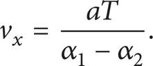
On the contrary, v_x = v₁.

The v_y and v_z are computed by the same way. Then we choose the minimum value v₂ from the v_x, v_y, and v_z. The determining transfer velocity is shown in Figure 9. The procedure of determining consecutive planning unit transfer velocity is called velocity preplanning. After the preplanning, the velocity planning is proposed.

Figure 9:

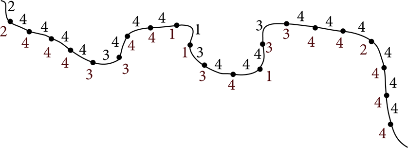
Velocity preplanning chart.

In Figure 9, the curve segment between two points is a planning unit. The digital number above the planning unit represents the velocity grade of the corresponding planning unit. The digital number on the transfer point represents the transfer point velocity.

7. Velocity Planning Algorithm of Whole Interpolation Trajectory

Considering the acceleration and deceleration ability of each planning unit, the target of the velocity planning should satisfy the following criterions:

the identification value digital number difference of two endpoints transfer velocity for all planning units should be lower than 1;

the velocity identification value on every transfer point after the velocity planning procedure should be lower than the corresponding velocity identification value after the preplanning procedure.

Criterion 1 ensures the correct inner acceleration/deceleration procedure for each planning unit. Criterion 2 ensures the processing accuracy of whole trajectory. From the above analysis, we can see the real velocity planning is changed to the velocity identification value planning.

In order to satisfy these two conditions and use the parallel strategy for computing every point velocity, we use the following “bubble” velocity planning method. Firstly, from the start point, the velocity identification value for consecutive two points is compared consecutively. For example, for point i, let point i + 1 velocity identification value be v_{i + 1} and point i velocity identification value v_i; if v_i⩾v_{i + 1} and 0⩽v_i − v_{i + 1}⩽1 (condition 1), both values of point i and point i + 1 are not changed; otherwise, if v_i > v_{i + 1} + 1 (condition 2), v_{i + 1} is not changed, but v_i = v_{i + 1} + 1; if v_i < v_{i + 1} (condition 3), v_i is not changed, but v_{i + 1} = v_i + 1. For comparison, every point pair can be computed in one thread; therefore, every point pair of whole trajectory can be computed simultaneously in GPU. This procedure is called one computation step. After finishing one computation step, the current computation step should be compared with the previous computation step. If the result is the same, the computation is finished and the velocity planning is completed. The results of all transfer point velocities are achieved. If the result is different, the computation procedure should continue. We will give an example in Figure 10 to illustrate the validity of the proposed algorithm. In this example, the velocity grades are limited to 5.

Figure 10:

Velocity identification value chart after velocity preplanning.

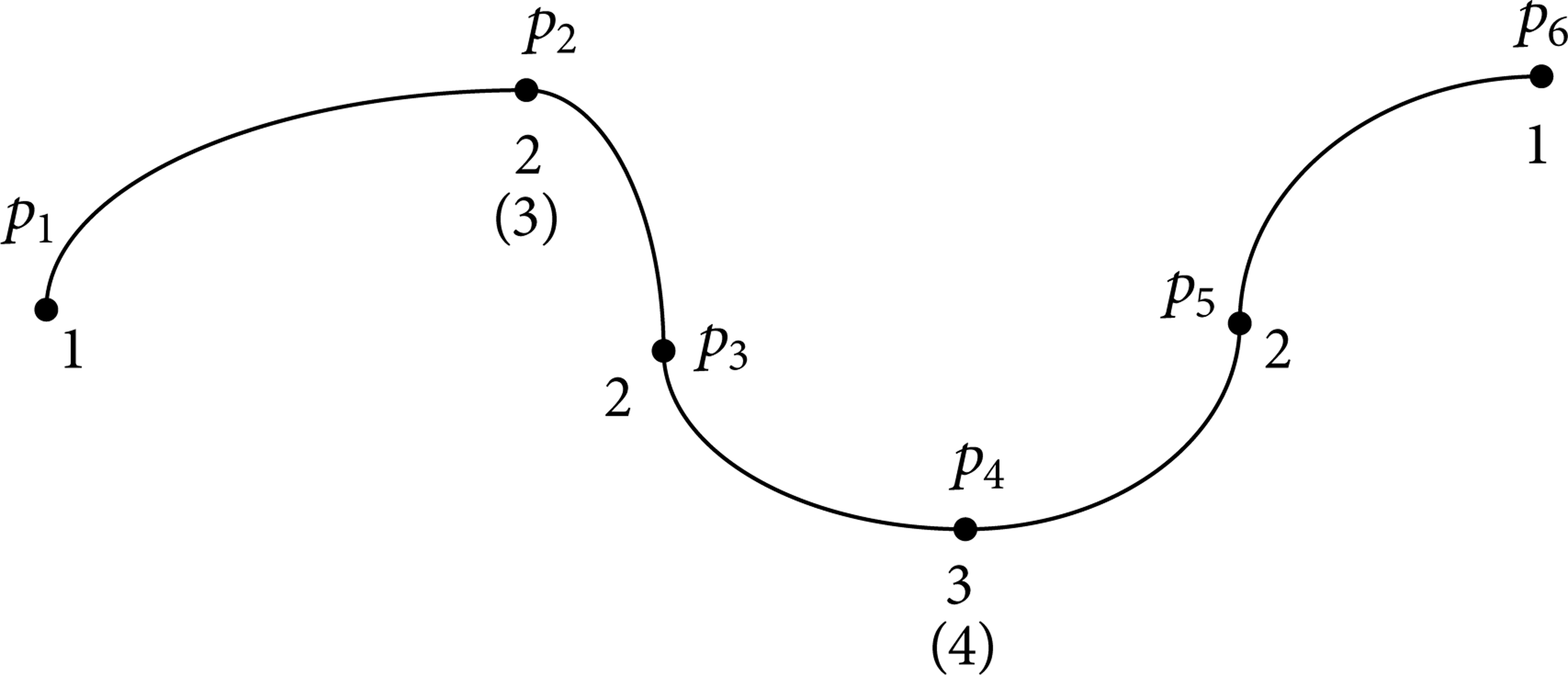
In Figure 10, six points from p₁ to p₆ are presented. The identification value under transfer points is the velocity grade value after the velocity preplanning procedure. The target of the velocity planning is to let all the transfer point velocity grade values satisfy the criterion 1 and criterion 2.

The velocity planning result after the first computing step is shown in Figure 11. From the figure, the planning point pair p₁p₂ thread satisfies condition 3; therefore, the velocity identification value of p₂ is changed to 2. The planning point pair p₂p₃ thread satisfies condition 2; the value of p₂ is changed again to 3. The planning point pair p₃p₄ thread satisfies condition 3; therefore, the value of p₄ is changed to 3. The planning point pair p₄p₅ thread satisfies the condition 2; therefore, the value of p₄ is changed again to 4. The planning point pair p₅p₆ thread satisfies condition 2; therefore, the value of p₅ is changed to 2. The end points before p₁ and after p₆ are computed the same way like above consecutively in their corresponding thread, respectively.

Figure 11:

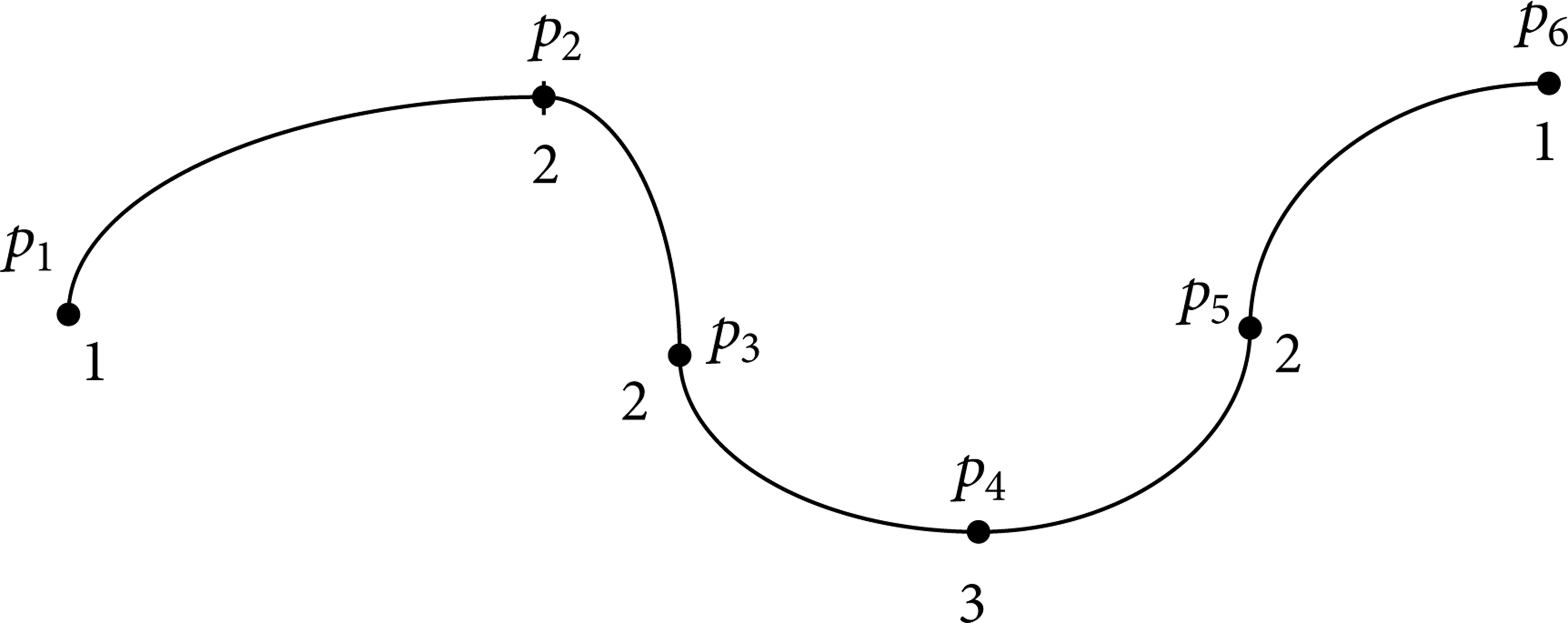
Velocity identification value chart after first computation step.

The velocity planning result after the second computing step is shown in Figure 12.

Figure 12:

Velocity identification value chart after second computation step.

From the above method, several computation steps are computed. From the example above, after three computation steps, the velocity of each point is the same as the second step, so the computation procedure is finished. The computation of all planning units and transfer points is finished and the result satisfies the two conditions. After determining the transfer velocity, for each planning unit, the acceleration is computed by the following equation, and then the velocity planning is finished and begins the trajectory interpolation procedure. a is computed as

a = \frac{v_{s}^{2} - v_{e}^{2}}{2 L} .

(15)

In this equation, v_s and v_e represent the start point velocity and end point velocity of a planning unit. L represents the planning unit length. In the real processing, when the interpolation velocity of two end points of one planning unit is obtained, the acceleration then also can be obtained by (15), and then we can feed these data to interpolation module. The flowchart of the above algorithm is shown in Figure 13. Here one key problem should be noted: in GPU, after finishing one computation step, all threads should be synchronized to one point, and then compute the next computation step.

Figure 13:

Velocity planning ith flowchart.

8. Simulation and Experiment Results

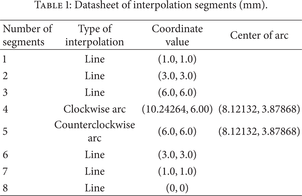
The parameters in experiment are as follows. The interpolation period T = 1 ms, time constant t₀ = 1000.0 ms, the maximal velocity which the system constricted is V_th = 500.0 mm/min, and the maximal acceleration which the system constricted is a_max = 25.0 mm/s²; because the algorithm introduced the arc interpolation, the whole interpolation processing is restricted in the x-y plane. The start point of interpolate is (0, 0) Which is used to compute the vector angel of space linesand the data of whole path segments are in Table 1.

Table 1:

Datasheet of interpolation segments (mm).

Number of segments	Type of interpolation	Coordinate value	Center of arc

1	Line	(1.0, 1.0)
2	Line	(3.0, 3.0)
3	Line	(6.0, 6.0)
4	Clockwise arc	(10.24264, 6.00)	(8.12132, 3.87868)
5	Counterclockwise arc	(6.0, 6.0)	(8.12132, 3.87868)
6	Line	(3.0, 3.0)
7	Line	(1.0, 1.0)
8	Line	(0, 0)

From Table 2, when the maximum number of look-ahead segments N = 0, the look-ahead algorithm does not work. When N = 1, 2, 6, except the segment 8, other interpolation end point velocities are all not zero, so interpolation time is shortened greatly. The velocity of S-shape acc/dec look-ahead algorithm comparison graph is shown in Figure 15. From Figure 14(b) to Figure 14(d), the minimal velocity appears in end point of path segment 4. It is because, at the end point of this segment, the vector transferring angle is 180°, and this angle constricts the velocity. The acceleration curve under the condition of N = 1 is shown in Figure 15. From Figure 15(a), when using S-shape acc/dec in look-ahead algorithm, the velocity profile is smoother than the linear acc/dec which is shown in Figure 15(b) and it has no acceleration sudden change. So the whole interpolation processing becomes more flexible and continuous.

Table 2:

Corresponding table of look-ahead segment number and segment end point velocity (mm/min).

	Segment 1	Segment 2	Segment 3	Segment 4

N = 0	0.0	0.0	0.0	0.0
N = 1	205.9768	357.3392	376.9957	3.0
N = 2	205.9768	357.3392	377.0077	3.0
N = 6	205.9768	357.3392	377.0077	3.0

	Segment 5	Segment 6	Segment 7	Segment 8

N = 0	0.0	0.0	0.0	0.0
N = 1	357.7637	292.2969	206.9792	0.0
N = 2	376.0143	358.3434	206.9792	0.0
N = 6	376.0143	358.3434	206.9792	0.0

Figure 14:

Comparative figure of velocity with different number of look-ahead segment.

Figure 15:

Comparative figure of acceleration curve when N = 1.

Figure 16 is relation graph of the maximum number of look-ahead segments and interpolation time. From this figure, when N = 0, the total time of interpolation is 31636 ms; when N = 1, the total time is 7456 ms; when N = 2, 3, 4,…, the total time is 7208 ms. From this data, the look-ahead algorithm can greatly improve the interpolation efficiency and decrease the interpolation time. But when the maximum number of look-ahead segment increases, the interpolation time does not decrease notably. When the number is too large, the time is not saved, but the computation load is increasing very quickly. So, selecting an appropriate number of look-ahead segments is very important. Commonly the maximum number of look-ahead segments should be restricted under 10 pieces.

Figure 16:

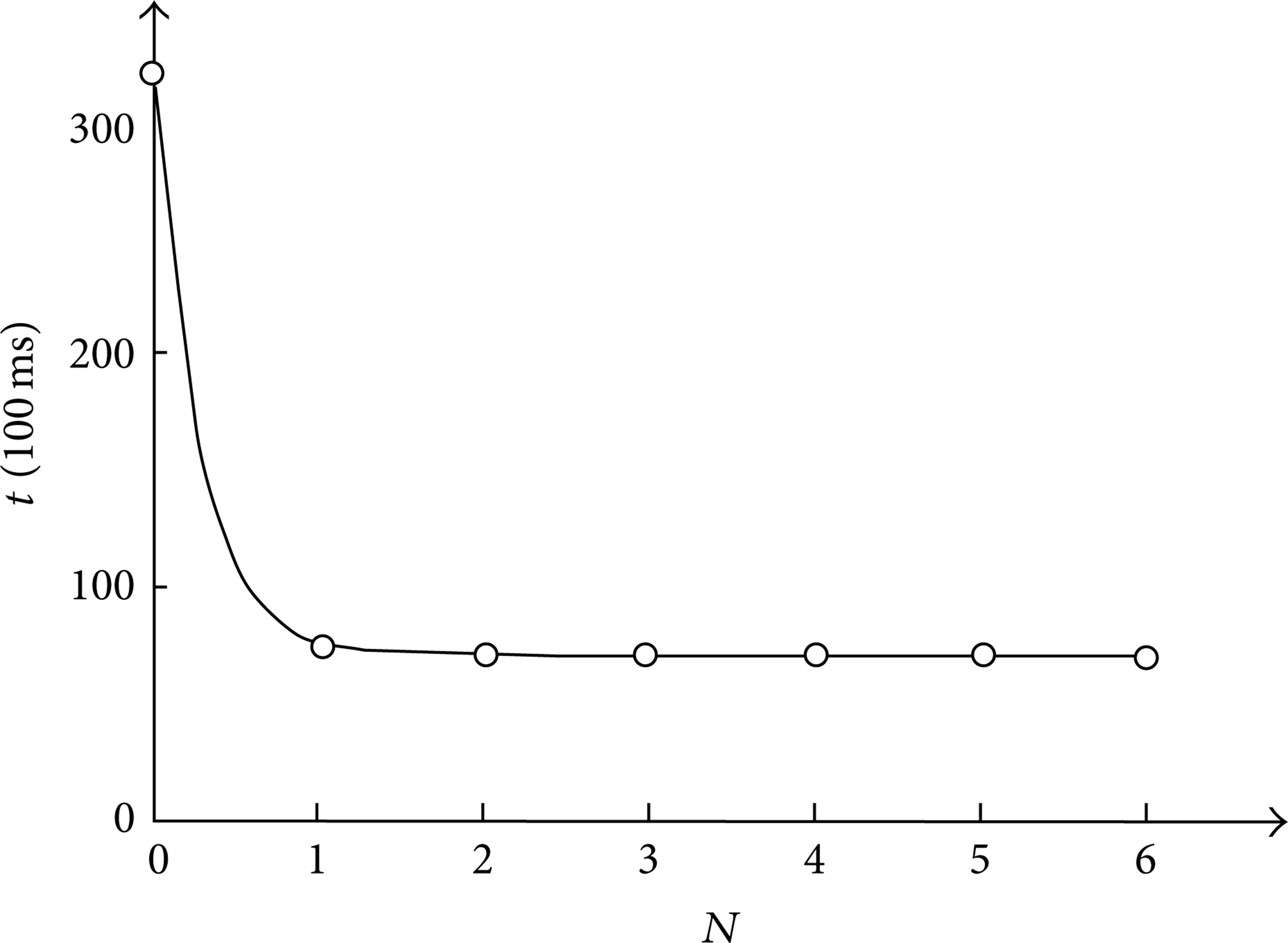
Machining time corresponding to the number of look-ahead segments.

Based on the new algorithm, the controller was developed on the basis of μc/os-II RTOS. It was programmed in C and compiled. The design environment consists of the source insight and ADS. Tests were carried out in the CAK6150N SYMS lathe, as illustrated in Figure 17. The CAK6150N lathe is a two-axis lathe. It possesses high-precision slideways that allow both two axes to reach a speed of up to 15 m/min. The workpiece of applying the new algorithm of interpolating is depicted in Figure 18.

Figure 17:

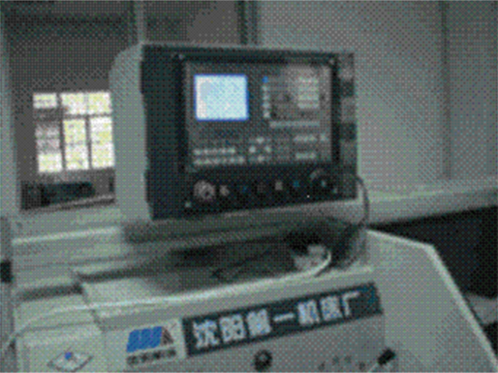
The test bed of the controller.

Figure 18:

The workpieces using the algorithm.

9. Conclusion and Future Work

In this paper, the GPU technology is introduced into CNC algorithm. The parallel structure model is constructed by CUDA, and a discrete planning unit look-ahead velocity control strategy is proposed. The GPU parallel computing mechanism of massive microsegments is discussed and, based on the research, a high-performance velocity planning algorithm is presented. This research result can highly raise the velocity planning and interpolation efficiency. This brand new solution can help improve the performance of CNC system dramatically.

In the future, we will investigate how to use this algorithm for real-time look-ahead NURBS velocity planning and also will find the way for closed-loop servo algorithm with the parallel computation.

Conflict of Interests

The authors declare that there is no conflict of interests regarding the publication of this paper.

References

Lin

M.-T.

Tsai

M.-S.

, and Yau

H.-T.

, “Development of a dynamics-based NURBS interpolator with real-time look-ahead algorithm,” International Journal of Machine Tools and Manufacture, vol. 47, no. 15, pp. 2246–2262, 2007.

Yau

H.-T.

Wang

J.-B.

, and Chen

W.-C.

, “Development and implementation for real-time lookahead interpolator by using Bezier curve to fit CNC continuous short blocks,” in Proceedings of the IEEE International Conference on Mechatronics (ICM '05), pp. 78–83, Taipei, Taiwan, July 2005.

Yau

H.-T.

and Wang

J.-B.

, “Fast Bezier interpolator with real-time lookahead function for high-accuracy machining,” International Journal of Machine Tools and Manufacture, vol. 47, no. 10, pp. 1518–1529, 2007.

Peng

, and Li

, “Look-ahead control in high feed rate NURBS curve interpolation,” Journal of Computer-Aided Design & Computer Graphics, vol. 18, no. 5, pp. 625–629, 2006.

Peng

Luo

, and Li

, “NURBS curve interpolation algorithm with the adaptation to machine tool kinetic character,” Journal of Huazhong University of Science and Technology, vol. 33, no. 7, pp. 80–83, 2005.

D.-S.

Yan

C.-L.

, and Li

C.-X.

, “An adaptive NURBS interpolator with real-time look-ahead function,” Journal of Shanghai Jiaotong University, vol. 40, no. 5, pp. 843–847, 2006.

Shi

Yang

, and Lv

, “Interpolation of continuous micro line segment trajectories based on look-ahead algorithm in high-speed machining,” The International Journal of Advanced Manufacturing Technology, vol. 37, no. 9–10, pp. 881–897, 2008.

Yang

C.-D.

, “Optimal feedrate control strategy for high-speed high-accuracy corner motions,” in Proceedings of the 32nd IEEE Conference on Decision and Control vol. 3, pp. 2517–2522, December 1993.

Wang

Y.-H.

Xiao

L.-J.

Zeng

S.-S.

Z.-Y.

, and Zhong

S.-B.

, “An optimal feedrate model and solution for high-speed machining of small line blocks with look-ahead,” Journal of Shanghai Jiaotong University, vol. 38, no. 6, pp. 901–904, 2004.

10.

and Zhao

, “Study on control algorithm for micro-line continuous interpolation,” China Mechanical Engineering, vol. 15, no. 15, pp. 1354–1356, 2004.

11.

Han

G.-C.

Kim

D.-I.

Kim

H.-G.

Nam

Choi

B.-K.

, and Kim

S.-K.

, “A high speed machining algorithm for CNC machine tools,” in Proceedings of the 25th Annual Conference of the IEEE Industrial Electronics Society (IECON '99) vol. 3, pp. 1493–1497, December 1999.

12.

Luo

F.-Y.

Zhou

Y.-F.

, and Yin

, “A universal velocity profile generation approach for high-speed machining of small line segments with look-ahead,” The International Journal of Advanced Manufacturing Technology, vol. 35, no. 5–6, pp. 505–518, 2007.

13.

Xiao

Wang

, and Wu

, “An optimal feedrate model and solution algorithm for a high-speed machine of small line blocks with look-ahead,” The International Journal of Advanced Manufacturing Technology, vol. 28, no. 9–10, pp. 930–935, 2006.

14.

Cao

W.-G.

and Chang

Q.-X.

, “A kind of arithmetic having the function of “look-ahead” in smoothly controlling,” Modular Machine Tool & Automatic Manufacturing Technique, vol. 9, pp. 56–59, 2005.

15.

Payne

J. L.

Sinnott-Armstrong

N. A.

, and Moore

J. H.

, “Exploiting graphics processing units for computational biology and bioinformatics,” Interdisciplinary Sciences: Computational Life Sciences, vol. 2, no. 3, pp. 213–220, 2010.

16.

Khanna

and McKennon

, “Numerical modeling of gravitational wave sources accelerated by OpenCL,” Computer Physics Communications, vol. 181, no. 9, pp. 1605–1611, 2010.

17.

Clark

M. A.

Babich

Barros

Brower

R. C.

, and Rebbi

, “Solving lattice QCD systems of equations using mixed precision solvers on GPUs,” Computer Physics Communications, vol. 181, no. 9, pp. 1517–1528, 2010.

18.

Dyken

Reimers

, and Seland

, “Real-time GPU silhouette refinement using adaptively blended Bézier patches,” Computer Graphics Forum, vol. 27, no. 1, pp. 1–12, 2008.

19.

Krishnamurthy

Khardekar

, and McMains

, “Optimized GPU evaluation of arbitrary degree NURBS curves and surfaces,” Computer-Aided Design, vol. 41, no. 12, pp. 971–980, 2009.

Discrete Planning Unit Look-Ahead Velocity Control Strategy and Parallelization Research Based on GPU

Abstract

1. Introduction

2. Whole Scheme of Parallel Velocity Planning Algorithm with GPU

3. Interpolation Geometry Elements Linking Vector Angle Model

3.1. Line to Line Condition

3.2. Line to Arc, Arc to Line, and Arc to Arc Conditions

4. Planning Unit and Velocity Grade

4.1. Planning Unit Concept

4.2. Planning Unit Length and Velocity Grade

4.3. Parallelized Velocity Grade Division Strategy

5. Interpolation Velocity in the Planning Unit

6. Velocity Determination of the Transfer Point between the Consecutive Planning Units

7. Velocity Planning Algorithm of Whole Interpolation Trajectory

8. Simulation and Experiment Results

9. Conclusion and Future Work

Conflict of Interests

References