On a Controlled Random Deployment WSN-Based Monitoring System Allowing Fault Detection and Replacement

Abstract

This paper presents a sensor random deployment scheme to monitor 2-dimensional areas for constraining applications while providing a mathematical control of the coverage quality it allows. In addition, useful techniques to detect and repair sensor failures are also added to provide system robustness based on this scheme. In particular, mathematical formulas are developed to express the probability of complete coverage when the environment characteristics are varying, taking into account the deployment parameters. Moreover, a methodology is presented to adapt this scheme to the need of various WSN-based monitoring applications. A simulation is also performed to show the efficiency of the developed strategy, highlight some of its features, and assess its impact on the lifetime of the monitoring system it serves.

1. Introduction: Need for Failure Detection and Repairing

With evolving sensor technologies, a growing number of sensors can be installed to architecture for the management and control of systems monitoring 2D areas. As the monitoring applications utilize the sensor data for alarming and decision, it is essential that (a) the data acquired by the sensors are accurate and reliable; (b) the sensing coverage quality is maximized at any time; and (c) the sensors are acting properly. One can notice, in particular, that sensor faults become more frequent compared to the architecture's lifetime and that the deployment techniques affect deeply the quality coverage of WSN.

The deployment strategies for WSNs providing area monitoring can be classified into three categories, namely, the static nodes placement with controlled deployment, the static nodes placement with random deployment, and the dynamic nodes placement with random deployment [1]. When it comes to the continuous monitoring of 2-dimensional areas (2D areas), all these techniques experience numerous drawbacks, either for their feasibility and the availability they provide or for the control they offer and the sensor lifetime they allow.

In particular, while the deployment strategies in the first class give optimal and guaranteed qualities of coverage in areas easy to access [2], these strategies fail hardly in accessible areas, since the sensors cannot be placed in positions chosen to ensure full coverage of the monitored area. On the other hand, the static node placement with the random deployment schemes operates by assuming that sensors are spread randomly in the monitored area [3, 4]. These schemes do not ensure total sensing coverage and radio connectivity to report all collected events, because the distribution of the sensors may not be uniform in the given area.

Strategies in the third class allow dynamic node placement with random deployment [5, 6], assuming that the deployed sensors are able to move within the monitored area. They mainly proceed through two steps. In the first step, the sensors are randomly spread in the monitored area. During the second step, the deficiency of coverage quality is compensated by commanding the sensors to move and change their positions to ensure the required quality of coverage. Monitoring applications using such strategies experience two major drawbacks. First, the node motion may cost a lot of energy. Second, the sensors may not be able to move properly to their new positions because of the nature of the monitored area and the obstacle irregularities they may face.

On the other hand, efficient monitoring systems should be able to address different constraints. In particular, they should provide (a) total sensing coverage of the monitored area or at least a large part of it, if the supported application is satisfied with it; (b) a wireless sensor network capable of relaying any detected event to the central station(s) in a real time manner; (c) the optimization of the energy consumption to provide longer sensor lifetime and reduce cost operation; and (d) the detection and repair sensor failures to keep the area continuously and properly covered.

In actual fact, a faulty sensor cannot perform its monitoring function properly, but, as an alternative, it may provide false information and induce erroneous decision, thus making the system unreliable or overconsuming energy [7]. Therefore, it is necessary to detect such failures and adapt the network to the new situation by running correcting actions such as sensor replacement. When the system is redundant, removing a failing sensor will not result in a loss of accuracy. However, if that is not the case or when the WSN has to operate for long time, a technique is needed for detecting, isolating and replacing/correcting a faulty sensor.

In this paper, a multistep method is proposed to deploy sensors and detect, isolate, and repair the sensors in the network when they get faulty. The main contribution of this paper is 4-fold.

• (i)

First, it builds a dropping scheme, from air, for example, capable of providing tight control on the landing positions of the deployed sensors based on a landing pattern taking into consideration the characteristics of dropping environment and the sensor transporter.

(ii)

Second, a mathematical model is developed to control the sensing coverage quality and the quality of network communication provided by the deployed WSN, using deployed data relaying nodes.

(iii)

Third, it builds a monitoring scheme for the energy depletion control and the management of failures of the deployed sensors while allowing fault predictions using rule-based strategies.

(iv)

Fourth, it builds mechanisms to replace (or repair) faulty sensors and increase the network availability and lifetime using the proposed deployment scheme.

In particular, the provided model and techniques allow planning the WSN design in a way that increases the probability of network connectivity by controlling a set of parameters including, but not limited to, the dropping point locations, the number of deployed data relaying nodes and their range, the dropping altitude, and the errors associated with the variation of the landing patterns.

The remaining part of this paper is organized a follows. Section 2 develops the proposed deployment scheme of WSN for 2D area monitoring applications, in its static form. Section 3 extends the mathematical model to integrate the variation of the parameters involving the environments and the sensor transporter. Section 4 discusses techniques for the detection and prediction of sensor faults. Section 5 discusses different uses of the proposed deployment scheme and gives rule-based strategies for the prediction. Section 6 discusses techniques for faulty sensor replacement. Section 7 develops a numerical simulation of a system based on the proposed scheme. Section 8 concludes this paper.

2. Controlled Random Sensor Deployment for Area Monitoring

Assume that a WSN is to deploy in a 2D area to monitor the occurrence of some events. Assume also that the WSN has a hierarchical structure, in the sense that it has three layers. The first layer is formed by basic sensor nodes (SNs). The role of a SN is to detect the occurrence of prespecified events that help in monitoring a given area and to report the collected data to near nodes in the second layer (eventually through other SNs).

The second layer is formed by communication nodes (CNs) acting as cluster heads for the SNs in the first layer and routing those sensor's reports to the nearest (sink) node in the third layer, as called analysis nodes (ANs). The ANs are responsible for (a) message analysis and prediction needed by the application served by the WSN; (b) sensor fault detection and localization; and (c) the energy management of all sensors in the WSN.

For the sake of coverage efficiency, the layer two nodes should constitute all the time a connected network. In the following two subsections, we define the major mathematical model to deploy sensors and determine their landing positions within the area to monitor and the deployment scheme, when the environment parameters do not vary during deployment. In addition, we assume that the nodes in layers 1 and 2 are dropped from air following a deployment pattern that we will formally define.

2.1. Deployment Patterns for Sensors

We define a sensor deployment pattern (SDP) as a 5-tuple $(q,\overrightarrow{V},\overrightarrow{F},n,\sigma )$ , where n is the number of sensors to deploy, q is the set of the landing positions of the sensors assuming that the sensors are one by one dropped from an airplane (e.g., the helicopter), $\overrightarrow{V}$ is the speed vector of the sensor transporter, $\overrightarrow{F}$ is the wind forces experienced by the sensors during dropping and falling down, and σ is a fixed interval separating two successive dropping times of the sensors.

We assume in the following that n is sufficiently small or that parameters $\overrightarrow{V}$ and $\overrightarrow{F}$ are unchanging during the deployment of the n sensors. To determine the landing area of the n sensors, we assume, for the sake of simplicity, that $\overrightarrow{F}$ has no vertical component ( $\overrightarrow{F}\hspace{0.17em}=(F_x,F_y,0)$ ) and that

$$\begin{array}{cc}& F_{x,b}\le F_x\le F_{x,f}-F_{y,s}\le F_y\le F_{y,s},\end{array}$$

(1)

where $F_{x,b}$ , $F_{x,f}$ , and $F_{y,s}$ are constant values controlling the flight feasibility of the sensor carrier (e.g., aircraft), knowing that $F_{x,b}\le 0,0\le F_{x,f}$ and $0\le F_{y,s}$ . These values define the maximum intensities of the headwind, back wind, and crosswind.

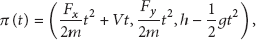
Using the fundamental principle of dynamics, one can see that the motion of a sensor dropped from position $A=(\mathrm{0,0},h)$ will follow the following path until its landing:

$$\begin{array}{cc}& \pi \left(t\right)=\left(\frac{F_x}{\mathrm{2}m}{t}^{\mathrm{2}}+Vt,\frac{F_y}{\mathrm{2}m}{t}^{\mathrm{2}},h-\frac{\mathrm{1}}{\mathrm{2}}g{t}^{\mathrm{2}}\right),\end{array}$$

(2)

where m, g, and V are the mass of the sensor, the universal acceleration, and speed of the airplane (assumed to be parallel to the x-axis) on dropping, respectively. Assuming that the dropping position is equal to $(\mathrm{0,0},h)$ , then the landing time and position of the first sensor can be given, respectively, by

$$\begin{array}{cc}& t_{\mathrm{1}}=\sqrt{\frac{\mathrm{2}h}{g},}\\ p_{\mathrm{1}}=\left(\frac{F_{x}h}{mg}+V{t}_{\mathrm{0}},\frac{F_{y}h}{mg},\mathrm{0}\right).\end{array}$$

(3)

Thus, it is easy to deduce that the landing time and position of the sensor j, $1\le j\le n$ , are given by

$$\begin{array}{cc}& t_j=t_{\mathrm{1}}+\left(j-\mathrm{1}\right)\sigma ,\\ p_j=\left(\frac{F_{x}h}{mg}+V{t}_j,\frac{F_{y}h}{mg},\mathrm{0}\right).\end{array}$$

(4)

Figure 1 depicts the landing area for possible values of V, $F_x$ , and $F_y$ . In this figure, the quantity $F_y$ is positive and the landing positions occur on parallel line to the x-axis.

Figure 1

Landing area.

Assume that the sensors have a sensing range equal to $R_s$ and a communication range equal to $R_c$ . To provide full monitoring, we first assume that

$$\begin{array}{cc}& \sigma V\le \mathrm{2}{R}_s\le R_c,\end{array}$$

(5)

meaning that after deployment, successive sensors can communicate with each other and that they guarantee sensing of the line between them. More precisely, we have the following result.

Proposition 1.

Let n sensors have a deployment pattern defined by $(q,\overrightarrow{V},\overrightarrow{F},n,\sigma )$ . After deployment, the area monitored by the deployed n sensors is the union, ${\bigcup }_{j\le n}Disk\mathrm{\hspace{0.17em}\hspace{0.17em}}(p_j,R_s)$ , of the discs sensed by sensor j, as located at $p_j$ , $\mathrm{1}\le j\le n$ .

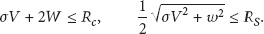
Moreover, if $\sigma V\le \mathrm{2}{R}_s\le R_c$ , the area contains a thick strip (or rectangle) containing the landing positions $p_j$ , $\mathrm{1}\le j\le n$ , and having a length L and a width W equal, respectively, to

$$\begin{array}{cc}& L=n\sigma V,\hspace{1em}\hspace{1em}W=\mathrm{2}\sqrt{R_s^{\mathrm{2}}-{\left(\frac{\sigma V}{\mathrm{2}}\right)}^{\mathrm{2}}.}\end{array}$$

(6)

In addition, the WSN is radio connected.

Proof.

Using (4), one can deduce that the landing point of the n sensors is given by

$$\begin{array}{cc}& p_j=\left(\frac{F_{x}h}{mg}+j\sigma V,\frac{F_{y}h}{mg},\mathrm{0}\right),\hspace{1em}\mathrm{1}\le j\le n.\end{array}$$

(7)

Thus, the distance between two successive landing points is equal to $\sigma V$ . Consequently, the n deployed sensors can communicate with each other, since $\sigma V\le R_c$ .

On the other hand, one can see that the sensing ranges of two neighboring sensorsj and $j+1$ intersect in two points $b_j$ and $c_j$ (as depicted in the lower part in Figure 2) given by

$$\begin{array}{cc}& b_j=\left(\frac{F_{x}h}{mg}+\left(j-\frac{\mathrm{1}}{\mathrm{2}}\right)\sigma V,\frac{F_{y}h}{mg}-\frac{W}{\mathrm{2}},\mathrm{0}\right),\\ c_j=\left(\frac{F_{x}h}{mg}+\left(j-\frac{\mathrm{1}}{\mathrm{2}}\right)\sigma V,\frac{F_{y}h}{mg}+\frac{W}{\mathrm{2}},\mathrm{0}\right).\end{array}$$

(8)

The distances between $\sigma V$ and $c_j$ and $b_j$ and $b_{j+1}$ are given, respectively, by W and $\sigma V$ . Therefore, the area covered by the n sensors contains the rectangle of length $n\sigma V$ and a width equal to W, as characterized by vertices $b_1,c_1,\dots ,b_n,c_n$ . Its axis passes by the landing points $p_j$ , $1\le j\le n$ .

Figure 2

Example of sensor deployment.

When $V\le 2R_s$ , one easily concludes that the thick strip is reduced to a line containing $p_1$ to $p_n$ .

2.2. Front-Sense Scheme

Using the result achieved in the previous subsection, we can define a deployment scheme, called frontier sensor (Front-Sense) deployment scheme, that is capable of providing total sensing coverage of a 2D area to monitor, using a connected 3-layer hierarchical WSN. To explain this, we assume, for the sake of simplicity, that the area to monitor is a rectangle and that the sensing deployment patterns operate under the same wind and flight conditions. More varying conditions can be easily considered.

The Front-Sense scheme is a 3-step process operating as follows.

Step 1 (decomposing the rectangle into landing pattern-based zones).

Assume that the length and the width of the rectangular area to monitor are equal to A and B, respectively, and that its south west vertex is (0, 0, 0). Let us partition it into strips of length A and width $R_s+(W/2)$ . The partition will need $\lceil (B+R_s)/(R_s+(W/2))\rceil$ strips, so that every point in the rectangular area will be in a sensing disk. We have denoted here the well-known ceiling function by $\lceil -\rceil$ . Figure 2 facilitates the presentation of the domain partition.

Step 2 (determining the sensor deployment pattern for every strip).

Let us assume that the sensor carrier is able drop the sensors from altitude h. Since the strips have equal lengths in the rectangle, the deployment patterns to deploy sensors in every strip will differ only on the droppings point to guarantee full sensing coverage of the rectangle. Let $(q_j,\overrightarrow{V},\overrightarrow{F},n_j,\sigma )$ be the pattern associated with the jth strip. Then, we set

• (i)

$n_j$ = $\lfloor A/\sigma V\rfloor$ ;

(ii)

$q_{\mathrm{2}k+\mathrm{1}}$ = ( $(\sigma V/\mathrm{2})$ − $(F_{x}h/mg)$ − $V{t}_{\mathrm{1}},(W/\mathrm{2})$ − $(F_{y}h/mg),h$ ) + ( $\mathrm{0},k(R_s$ + $(w/\mathrm{2})),\mathrm{0}$ ),   $k\ge \mathrm{0}$ ;

(iii)

$q_{\mathrm{2}k}$ = ( $(\sigma V/\mathrm{2})$ − $(F_{x}h/mg)$ − $V{t}_{\mathrm{1}},(W/\mathrm{2})$ − $(F_{y}h/mg),h$ ) + $(0,k(R_s$ + $(W/\mathrm{2})),0)$ , $k\ge \mathrm{1}$ .

The expressions are easy to set since the strips of odd order are similar, while the strips of even order are similar. Thus, the total number of dropped sensors is equal to the number of strips $(=\lceil (B+R_s)/(R_s+(W/2))\rceil )$ times the number of sensors per strip $(=\lfloor A/\sigma V\rfloor )$ .

Step 3 (computing the landing positions of sensors to deploy).

The landing positions of the first sensors in the first strip and the second strip are given, respectively, by

$$\begin{array}{cc}& p_{\mathrm{1,1}}=\left(\frac{\sigma V}{\mathrm{2}},-\frac{W}{\mathrm{2}},\mathrm{0}\right),\hspace{1em}\hspace{1em}{p}_{\mathrm{2,1}}=\left(\mathrm{0},R_s,\mathrm{0}\right).\end{array}$$

(9)

The positions of the deployed sensors in the first and second strip are obtained from $p_{\mathrm{1,1}}$ and $p_{21}$ using transaction vectors

$$\begin{array}{cc}& k\left(\sigma V,\mathrm{0,0}\right),\hspace{1em}\mathrm{1}\le k\le n.\end{array}$$

(10)

The positions of the remaining sensors are deduced from the positions of the sensors in the first and second strip using translation vectors

$$\begin{array}{cc}& k\left(\mathrm{0},-\mathrm{2}\left(R_s+\frac{W}{\mathrm{2}}\right),\mathrm{0}\right),\hspace{1em}\mathrm{1}\le k\le \lfloor \frac{n}{\mathrm{2}}\rfloor .\end{array}$$

(11)

Figure 2 depicts the rectangular area to monitor and its partitioning into sensing disks.

To monitor areas with general forms, we first construct the smallest rectangle containing the given area. Then, we can decompose the rectangle into strips with the width considered in Step 1. The strips are then shortened to the right size by considering the intersection between the area and the strips. The deduced strips have variable lengths. This makes the deployment patterns assigned to each strip different in the number of sensors they handle and the landing points. Step 1 in Front-Sense scheme can be modified accordingly, and the number of sensors is deduced for every strip. Figure 3 depicts an example of area coverage area by five strips.

Figure 3

Example of covered area.

3. Coping with Environment Variations

Several assumptions have been made in the previous sections to make Front-Sense scheme presentation and explanation easy to understand. Assumptions have mainly included the airplane velocity, the dropping altitude, the wind intensity, the area form, and the geographic features of the area. In the following, we address these issues under two hypotheses: low variation and modeled variation.

3.1. Adapting the Scheme to Slow Variations: Pattern Management

To cope with the variation of the wind speed, one can choose to measure more often the wind speed and deploy the sensors in a strip using as many sensor deployment patterns as possible, in the sense that the number of sensors in a pattern is fixed based on an estimated period of invariability of the wind speed. To implement this, let us assume that the wind speed statistics show that if the wind measurement is made at an instant $t_0$ , then the variation of the wind intensity is negligible in the time interval ${[t}_0,t_0+\epsilon ]$ , for given positive ε. Then, the number of sensors to deploy during this interval using a pattern should be equal to $\lfloor \epsilon /\sigma \rfloor$ . After dropping these sensors, a deployment pattern is reconstructed to continue dropping sensors in the strip, taken into consideration a new measurement. The estimation of ε can be made using variation methods including averages made on historical data.

One can notice, however, that using multiple patterns per strip would make the width of the strip slightly vary from one pattern to another. This should be taken into consideration when proceeding with the next strip by placing appropriately this strip. In addition, adapting properly the control imposed by the inequality $\sigma \le \lceil R_s/V\rceil$ would guarantee the continuation of the sensing coverage.

To cope with the dropping altitude, area flatness, and area vegetation (i.e., the variation of h), we can assume that the variation h is negligible in a given time interval ${[t}_0,t_0+\epsilon ]$ , for given positive ε. The above technique can be used to determine various deployment patterns and measurements of h; however, one can notice that while the variation of the airplane speed only affects the x-position of the landing points (by a maximum value $\epsilon ·V$ in the time interval ${[t}_0,t_0+\epsilon ]$ ), the variation of the altitude h affects both the x-position and y-position of the landing points.

Consequently, the landing positions can be adapted appropriately, assuming that the geography of the area to monitor is not so abrupt. Upon the occurrence of sudden changes in the geography of the area, the recomputation of the pattern may be triggered.

On the other hand, one can be convinced that to cope with the wind speed variation, a technique similar to the one used for h can be implemented, provided that this variation is limited in time and intensity.

3.2. Coping with Fast Variable Parameters

We consider in this subsection only the case where the wind intensity is varying under a uniform model. Assume now that n sensors are to be dropped, from air, using the following sensor deployment pattern:

$$\begin{array}{cc}& \left(\left(\mathrm{0,0},h\right),\left(V,\mathrm{0,0}\right),\left(F_x,F_y,\mathrm{0}\right),n,\sigma \right).\end{array}$$

(12)

Assume, in fact, thatduring interval of time $[0,\sigma V]$ , $(F_x,F_y)$ is uniformly distributed inthe rectangle

$$\begin{array}{cc}& \left[F_{\mathrm{1}}-a,F_{\mathrm{1}}+a\right]\times \left[{F_{\mathrm{2}}-b,F}_{\mathrm{3}}+b\right],\end{array}$$

(13)

where a and b are positive numbers and $F_1$ and $F_2$ represent average values of the x-intensity and y-intensity of the wind. Using (4), the dropping positions of the jth sensor will occur in a rectangle ${Sq}_j$ , $j\le n$ , centered at

$$\begin{array}{cc}& p_j=\left(\frac{F_{\mathrm{1}}h}{mg}+j\sigma V,\frac{F_{\mathrm{2}}h}{mg},\mathrm{0}\right).\end{array}$$

(14)

A simple computation of ${Sq}_j$ shows that

$$\begin{array}{l}{Sq}_j=\left[\frac{\left(F_1-a\right)h}{mg}+j\sigma V,\frac{\left(F_{\mathrm{1}}+a\right)h}{mg}+j\sigma V\right]\hfill \\ \times \left[\frac{\left(F_2-a\right)h}{mg},\frac{\left(F_{\mathrm{2}}+b\right)h}{mg}\right].\hfill \end{array}$$

(15)

The surface of ${Sq}_j$ is given by $4ab{(h/mg)}^2$ and the actual landing is uniformly distributed in ${Sq}_j$ . Let S be a strip of width w and length $n\sigma V$ axed on the points $p_j$ , $j\le n$ , and denote in the sequel that

$$\begin{array}{cc}& \mathrm{2}\frac{ah}{mg}=w,\hspace{1em}\hspace{1em}\mathrm{2}\frac{bh}{mg}=W.\end{array}$$

(16)

The subsequent results estimate the quality of communication and sensing coverage of Front-Sense scheme based on the concept of deployment pattern. Figure 4 depicts the strip, the sensing range of sensor j, and clarifies the conditions provided in the first result.

Figure 4

Random deployment on a strip.

Proposition 2.

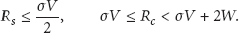
Consider the above notations and assume that the communication range and sensing range of the n deployed sensors in S satisfy the following conditions:

$$\begin{array}{cc}& {\sigma V+\mathrm{2}W\le R}_c,\hspace{1em}\hspace{1em}\frac{\mathrm{1}}{\mathrm{2}}\sqrt{{\sigma V}^{\mathrm{2}}+w^{\mathrm{2}}}\le R_S.\end{array}$$

(17)

Then, S is totally sensed by the n sensors, and the n sensors are able to communicate with each other.

Proof.

We first notice that the condition on $R_c$ shows that the distance between sensors j and $j+1$ is lower than $R_c$ , whatever is their landing points in squares ${Sq}_j$ and ${Sq}_{j+1}$ . In fact, the largest distance between points in squares ${Sq}_j$ and ${Sq}_{j+1}$ is lower than $\sigma V+2W$ .

Now, let us consider the intersection of the sensing range of sensors j and $j+1$ . The intersection is reduced to two points $b_j$ and $c_j$ given by

$$\begin{array}{cc}& b_j=p_j+\left(\frac{\sigma V}{\mathrm{2}},\frac{w}{\mathrm{2}},\mathrm{0}\right),\\ c_j=p_j+\left(\frac{\sigma V}{\mathrm{2}},-\frac{w}{\mathrm{2}},\mathrm{0}\right).\end{array}$$

(18)

Considering the condition on $R_s$ , one can deduce easily that $b_j$ and $c_j$ are the border of S and thus that S is completely sensed by the n sensors.

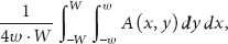
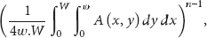
The following result computes, in more general settings, the probability that the n sensors are able to sense and communicate.

Theorem 3.

Consider the above notations and assume that the communication range and sensing range of the n deployed sensors in S satisfy the following conditions:

$$\begin{array}{cc}& R_s\le \frac{\sigma V}{\mathrm{2}},\hspace{1em}\hspace{1em}{\sigma V\le R}_c<\sigma V+\mathrm{2}W.\end{array}$$

(19)

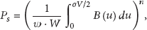
Then

• (1)

the probability that the n sensors are able to communicate with each other is given by

$$\begin{array}{cc}& P_c={\left(\frac{\mathrm{1}}{{\mathrm{4}\left(w·W\right)}^{\mathrm{2}}}{{\displaystyle \int }}_{-W}^W{{\displaystyle \int }}_{-w}^{w}A\left(x,y\right)dy\hspace{0.17em}dx\right)}^{n-\mathrm{1}},\end{array}$$

(20)

where $A(x,y)$ is the area covered by ${Sq}_{j+\mathrm{1}}$ and the disk of radius $R_c$ centered on $(x,y,0)$ in ${Sq}_j$ ;

(2)

the probability $P_s$ that main axis of S is totally sensed by the n sensors is given by

$$\begin{array}{cc}& P_s={\left(\frac{\mathrm{1}}{w·W}{{\displaystyle \int }}_{\mathrm{0}}^{\sigma V/\mathrm{2}}B\left(u\right)du\right)}^n,\end{array}$$

(21)

where   $B(u)$ is the area covered by ${Sq}_j$ and the disk of radius $R_s$ centered on $(u,\mathrm{0,0})$ segment $p_j{p}_{j+\mathrm{1}}$ .

Proof.

To demonstrate the first statement of the theorem, we only need to consider that the probability $P_{c,j}$ that sensors j and $j+1$ communicate together is given by

$$\begin{array}{cc}& \frac{\mathrm{1}}{\mathrm{4}w·W}{{\displaystyle \int }}_{-W}^W{{\displaystyle \int }}_{-w}^{w}A\left(x,y\right)dy\hspace{0.17em}dx,\end{array}$$

(22)

since $(x,y,0)$ can be everywhere in ${Sq}_j$ . This can be easily seen when noticing that $A(x,y)/(4w·W)$ is the probability that sensors j and $j+1$ can communicate together, knowing that sensor j is placed on $(x,y,0)$ . Figure 4 depicts ${Sq}_j$ , the small square around $(x,y,0)$ , and $A(x,y)$ .

The connectivity of the sensors in the strip is then equal to

$$\begin{array}{cc}& {\left(\frac{\mathrm{1}}{\mathrm{4}w.W}{{\displaystyle \int }}_{\mathrm{0}}^W{{\displaystyle \int }}_{\mathrm{0}}^{w}A\left(x,y\right)dy\hspace{0.17em}dx\right)}^{n-\mathrm{1}},\end{array}$$

(23)

since, to get this, sensors j and $j+1$ should be able to communicate for every $j\le n-1$ . Thus,

$$\begin{array}{cc}& P_c={\displaystyle \prod }_{j=\mathrm{1}}^{n-\mathrm{1}}{P}_{c,j}.\end{array}$$

(24)

Now let $(u,\mathrm{0,0})$ be a point on the segment $p_j{p}_{j+1}$ , let and $B(u)$ be the intersection of ${Sq}_j$ and the disk of radius $R_s$ centered at $(u,\mathrm{0,0})$ . Since $R_s\le (\sigma V/2)$ , the point $(u,\mathrm{0,0})$ can only be covered by a sensor in ${Sq}_j$ . The probability that a sensor in ${Sq}_j$ covers $(u,\mathrm{0,0})$ is equal to $B(x)/4wW$ . Thus, we have

$$\begin{array}{cc}& P_{s,j}=\frac{\mathrm{1}}{\mathrm{4}w·W}{{\displaystyle \int }}_{\mathrm{0}}^{\sigma V/\mathrm{2}}B\left(u\right)dx.\end{array}$$

(25)

This concludes the theorem, since

$$\begin{array}{cc}& P_s={\displaystyle \prod }_{j=\mathrm{1}}^{n-\mathrm{1}}{P}_{s,j}.\end{array}$$

(26)

4. Sensor Failure Detection and Prediction

Amongst the challenges that WSN-based monitoring applications are facing, one can mention the quality of service (QoS) provided by the network and the lifetime of the network. The latter depends largely on the energy consumption of sensors composing the network. Most important concerns of QoS include (a) the quality and the amount of the information that can be collected and analyzed about the observed objects; (b) the detection of sensor faults and the tolerance of the monitoring system to these faults; and (c) the quick recovery from a fault. In fact, a sensor fault can be defined as a deviation from the expected model of the function the sensor is assumed to perform.

Faults can occur in different layers of WSN, but most commonly they occur at the physical layer, since sensors are most prone to malfunctioning and energy depletion. Major faults include calibration systematic faults, random faults from noise, energy exhaustion, and complete malfunctioning [8–10]. Calibration faults appear as drifts throughout the lifetime of a sensor node. Random noises induce random unwanted variations in the data reporting on the events detected by the sensors. Energy exhaustion occurs when batteries fail to provide the needed energy for detection and reporting.

4.1. Fault Classification

Sensor faults can be defined through two overlapping viewpoints: data-centric and system-centric faults [8]. Faults in the first category can be observed in readings through the effect they produce in data. Faults in the second point of view are observed with physical malfunction, environment conditions’ modifications, and inconsistencies of factors that are not expected to change throughout the lifetime of sensor.

The most common classes of sensors that have been used extensively in 2D area monitoring implement functions for the sensing of temperature, humidity, light, chemical elements, and mobile objects. Major features for these sensors include sensor location, environment characteristics, system features (e.g., calibration, detection range, reliability, and noise), and date features (e.g., statistical measures, gradients, and distance from other readings).

In the sequel, we only consider the data-centric viewpoint since one can assume, for sensor-based monitoring, that all the features revealing faults can be deduced from the reports transmitted to the sink for analysis. In particular we distinguish the following features/faults.

Temporal Gradients. We define a temporal gradient to be a rate of change, of a feature (or parameter), larger than expected over a short time window, despite what can be the value of the feature afterwards. In general, the determination of gradient is based on environmental context and models of the physical phenomenon to observe. It is a grouping of several data reports (or data samples) and not one isolated event. An example of gradient can be light intensity going through sudden and large changes.

Crossing Boundaries. A fault or the proximity of occurrence of a fault can be controlled by numerical metrics whose values are crossing a threshold. The crossing is typically an isolated sample or a sensor that significantly deviates from their expected temporal or spatial models. In particular, a temperature exceeding a high value for a point in a forest may reveal the occurrence of fire around that point. On the other hand, the level of remaining energy reported for a battery, powering a sensor, may show that the battery is running out of charge.

Zero Variations. Some faults can be defined as a series of data values (reported to the sink) that experiences zero or almost zero variation for a period of time greater than expected. Thus, a zero variation fault shows a constant value for a large amount of successive reported data. This value can be located outside, or within, the range of the expected values of the observed parameter. In particular, it can be either very high or very low.

High Noise. Noise is commonly expected in sensor data communication. Nonetheless, an abnormally high amount of noise may be an indication of a sensor problem. We define a noise fault to be sensor data exhibiting an unexpectedly high amount of variation. In fact, high noise may be due to a hardware failure or low energy batteries. Despite the noise, noisy data may still provide information regarding the phenomenon under monitoring.

Missing Data. A missing data requested by the monitoring protocol or a specific request sent by the sink may be a sign of fault. Moreover, missing periodic data for a relative period of time as expected can reveal a faulty sensor. Often, missing data is caused by the sensor generating the expected data of intermediate sensors in charge of relaying the data.

4.2. Fault Detection

Let us consider only the detection of sensor faults in WSN-based monitoring applications of 2D areas. Various works have addressed this issue assuming that a large set of hypotheses can be made on the sensor network and the data for sensor fault detection [9]. Among the major assumptions, we consider the following. First, all sensor data should be forwarded to a central node (or sink), where the event processing is performed. Second, all data received by the sink is not corrupted by any communication error. Third, no security attack is targeting the data flowing through the network, its components, or its sensors when fault is occurring.

We also consider the following two requirements to be fulfilled.

• R1:

an event detected by a sensor will be detected in the near future, either by a neighboring sensor or by the same sensor. In the latter, the attached data should be different.

R2:

sensors reporting an event should be appropriately identified and correctly localized and the localization errors are bounded.

Sensors deployed for monitoring applications using our deployment scheme comply with these requirements. In fact, events collected for the applications we consider are related to moving objects in a 2D area (e.g., fire in a forest and intruders of the frontier line). Collected events are time-stamped and include varying data (such as temperature or intruder position). Let us notice however that the location of a sensor is determined by the deployment pattern used to deploy it. The location is nothing but the center, $p_j$ , of the square where it falls down. The location error is controlled by the size of this square.

Let us now present the main two detection methods of sensor faults, as denoted by variance-based detection and profile-based detection. While the fist technique builds for resource consumption and predicts time of their exhaustion, the second handles the variance of a feature characterizing a given fault among the aforementioned list of faults. Both methods follow the same approach for fault detection: they first characterize the “normal” behavior of sensor reported data; then they identify the occurrence of significant deviations as faults and finally give some predictions on the related fault. However, for the sake of simplicity we consider only one type of fault for each method. In particular, we consider energy depletion and the temporal gradient.

Loss of Energy. Let n be an integer (equal to 3 or 4, in general). Let us assume that a sensor in the WSN has to send a message $m_i$ , $i\le n,$ any time its energy reaches a level equal to $(i/n)E$ , where E is the initial energy level of the sensor. The message is time-stamped and contains the identity of the sensor and its location. Upon receipt, the central station verifies the accuracy of the attached data, computes the depletion time, and estimates the remaining lifetime of the sensor. If $i=n-1$ , then a request for the replacement of the failing sensor is sent.

The following section discusses the rules followed to monitor the energy consumption and the prediction of loss in the case of border surveillance.

Temporal Gradient. Let us assume selected a window N, a standard deviation σ, and threshold $\text{Th}$ , on the arrival of a message reporting on an event observed by a sensor s. The sink node computes the standard deviation of sample readings within a window N. If it is above a threshold $\text{Th}$ , the samples are compared with the simples of the neighboring sensors. If no correlation can be established in a corrected manner, the selection of N, σ, and $\text{Th}$ is performed through rules involving the nature of the 2D area, the application using the WSN, and the feature characterizing the fault.

Variation techniques have been developed to provide good estimation of the different parameters involved in the detection of faults [11]. While our method uses heuristics for detecting and identifying the fault types and exploits statistical correlations between sensor measurements to generate estimates for the sensed phenomenon based on the measurements of the same phenomenon at other sensors and reduce false positives, other techniques are time-series-analysis-based or learning-based [12] techniques.

5. Adapting the Front-Sense Scheme for Monitoring Uses

Various monitoring applications may benefit from the use of our deployment scheme. Among these applications, we consider in this section two special examples, namely, the border surveillance and wildfire sensing. We, first, present the architectural issues of the network that will be used for these applications. We will present the hierarchy of the network and the major functionalities.

The network is formed by three layers built on the following three types of node.

• (i)

The sensor nodes (SNs) constitute the first hierarchical level. They are in charge of detecting the occurrence of an event of importance to the monitoring application. They also collaborate to relay the information gathered to the next layer in an optimized manner. SNs are assumed to know approximately their location information.

(ii)

The relaying nodes (RNs) constitute the second hierarchical layer of the network. The RNs main task is to collect the data gathered by the SNs and collaborate to relay it to the next layer. They may include intelligent functions to help in handling energy consumption, coverage estimation, and fault detection.

(iii)

The analysis nodes (ANs) form the third layer. Their function is to receive the events detected at first layer and correlate them, analyze and predict failures, operate object tracking, and coordinate actions.

5.1. Country Border Surveillance

A country border surveillance application monitors either an area on the country border or a borderline. This type of applications is becoming a serious concern due to the increase of the risks of illegal border crossings aiming at controlling unauthorized importation of goods or terrorism actions. Border surveillance can be performed using specialized WSNs appropriately deployed. Typically, WSNs within these applications are interconnected and have to report on any event related to crossings. For this, they should provide efficient monitoring and a certain coverage level of the 2D area (or line) of interest, since the coverage can be total (when the 2D area is completely sensed) or partial (when, for example, it is done through several thick lines in the 2D area), [13, 14].

The deployment scheme described in the previous sections can be used to provide total or partial coverage of cross-border actions, using sensor capable of detecting individual and animal motions. Indeed, total coverage of the network first and second layers in the 2D area can be realized using RDAM as operating according to Figure 2. A partial coverage can be achieved by guaranteeing the surveillance of several lines parallel to the border line. In both cases, the altitude and speed of the airplane, the wind speed, the sensing range, and the communication range of the nodes can be selected in way that the probability of total coverage can be as high as needed.

Rules to handle sensor faults in border surveillance handle mainly energy depletion, sensor location, and location of detected object. Rules include the following.

Energy Level Reporting Rule. Let $0\le n$ and $L_0$ be the initial level of energy of a sensor; then the sensor should send a message $m_i$ every time its energy goes down to $L_i={(i/n)L}_0$ , $i\le n$ , indicating the time noticing this fact. Accordingly, the sink node receiving the messages adapts the lifetime of the battery and the remaining lifetime ${\tau }_i$ .

One should have ${\tau }_i>{\tau }_{i+1}$ ; otherwise, a fault is noticed.

Energy Threshold Crossing Rule. If the reported level of energy ${\tau }_i$ is lower than a threshold $E_0$ , then the sink deduces that the sensor is entering a fault state.

Replacement Rule. If the reported level of energy ${\tau }_i$ is lower than a given threshold $E_1$ , then the sink deduces that the sensor is getting to a faulty state soon. It then should trigger a sensor replacement procedure.

Object Location Rule. Knowing the limited speed of the detected object and that the positions of the deployed sensors are known with reduced errors, then important variations of observed object positions reveal faulty positioning function on a sensor.

5.2. Wildfire Sensing

Monitoring the location and speed of advance of the fire front wave is a critical task to fight against wildfire and help in optimizing the allocation of firefighting resources while maintaining safety of the firefighters. A WSN-based fire monitoring system is a 2-area deployed fire alarm system that is able to remotely report the location of its components and the presence of a fire in their vicinity. Indeed, a wildfire can be monitored using multiple sensors that are able to detect smoke, carbon monoxide, methyl chloride, rapid temperature increases, windy speed, and other physical phenomena related to the occurrence and propagation of a fire. The use of sensors reduces the likelihood of false alarms without excessive complexity to the WSN. The data gathered is typically transmitted by radio in real time to firefighters equipped with radio receivers or to a sink, called the fire command center. The sensor can be dropped from air or be manually placed by firefighters over a predefined 2D area.

Monitoring wildfire presents the problem of wide covered areas requiring the transmission of a large amount of information through the network with the risk of significant energy consumption and hence limiting the lifetime of the network. Particularly, energy is crucial for the wildfire sensing because of the complexity of maintenance of the sensors and the replacement of empty batteries due to the difficulty of access to these sensors, in general. Another problem needs to be tackled by these systems; it is the fading effect. Due to the presence of vegetation, this leads to important problems such as the shadowing phenomenon.

An efficient wildfire monitoring should propose an optimized design capable of providing energy conservation, consideration of the quality of transmission, and spatial localization techniques for choosing the routing protocol. A solution based on DRAM can be built using the aforementioned 3-layer architecture, where we assume that detection is not made on image processing to detect energy related faults [15].

Fault detection can be done using the aforementioned rules for the faults related to energy. A library of rules for reporting faults can be built on the available models developed for the evolution, propagation, of smoke and temperature. These rules use contradictions or repeated errors observed on the reported information by neighboring sensors. Examples of rules include the following rules dealing with temperature.

Irregular Variation of Temperature Rule. A sensor, ψ, detecting that the temperature has exceeded a threshold τ starts sending messages every δ seconds to report on the temperature and its neighbors are requested to report on the temperature in their vicinity. If the reported values are not coherent then sensor ψ is experiencing a fault. For this, coherence cases can be distinguished.

Regular Variation of Temperature Rule. A sensor, ψ, detecting that the temperature is increasing and has exceeded a value η lower than the sensor breaking temperature ${\tau }^{\prime }\hspace{0.17em}(\eta <{\tau }^{\prime })$ starts sending messages every time the temperature exceeds ${\tau }_i=(i/n)({\tau }^{\prime }-\eta )$ , for a prespecified n. Using these messages, the sink node(s) is able to estimate the remaining time to reach ${\tau }^{\prime }$ .

6. Deployment-Based Repairing of Sensor Failures

In this section, we develop techniques using our deployment scheme to plan the replacement of faulty sensors or sensors on their way to a faulty state. In addition, we will discuss techniques allowing reactive actions to reduce the loss of coverage (sensing or communication) due to the occurrence of faults.

6.1. Proactive Sensor Replacement

Replacement of sensors for a given monitoring application based on DRAM is built using a 3-phase process in charge of (a) the detection of faulty sensors; (b) the prediction of the time of occurrence of faults; and (c) the computation of new deployment patterns and instant of sensor dropping. The detection of faults can be achieved through a library of rules, similar to those discussed previously, taking into account the nature of the activity to monitor and the models governing the evolution of fault related parameters.

The prediction of fault occurrence is performed based on two things, the collection of messages helping in analyzing the temporal evolution to fault and a theoretical model governing evolution of related parameters, if any. The generation of the first message is often triggered when a threshold is reached, while the following messages are sent, by the concerned sensor or by its neighbors, on a time-based or event-based manner.

Upon receipt of the messages, the sink node can configure the related model, if any, and adapt to the reality of the situation to deduce the time to live before the occurrence of the fault. The actions in this step have been discussed in the previous section in the case of energy loss and temperature evolution.

On the other hand, the computation of new deployment patterns and instant of sensor dropping can be operated as follows: let $(q,\overrightarrow{V},\overrightarrow{F},n,\sigma )$ be a deployment pattern that has been used to deploy sensor and let ${(p_j)}_{j\le n}$ be the reference landing locations of the n sensors, as computed in Section 2. Assume now that p among the n sensors are faulty and need to be replaced and let $p_{j1},\dots ,p_{jp}$ be the reference position of the faulty sensors. Then, a replacement deployment pattern, denoted by $(q^{\prime },\overrightarrow{V^{\prime }},\overrightarrow{F^{\prime }},p,\Sigma )$ , should be used to plan the replacement. The components of this pattern are defined and computed as follows:

• (i)

$q^{\prime }$ is the first dropping position of the p replacing sensors;

(ii)

$\overrightarrow{V^{\prime }}$ is the speed of the airplane during the dropping period;

(iii)

$\overrightarrow{F^{\prime }}$ is wind intensity during deployment, assuming that it varies a little;

(iv)

$\Sigma =\{{\sigma }_1,\dots ,{\sigma }_j\}$ is a set of time values separating the dropping times of the successive sensors.

Assume that the period of dropping is selected so that the altitude h (in $q^{\prime }$ ) and the speed $\overrightarrow{V^{\prime }}$ can be chosen in a way allowing the following conditions.

• (1)

The reference lending position of sensor k, $p_k^{\prime }$ , $k\le p$ , is very close to $p_{jk}$ .

(2)

The actual landing of sensor $\mathrm{1}$ , $p_{\mathrm{1}}^{\prime }$ , is a rectangle close to the rectangle delimiting the actual landing point to $p_{j\mathrm{1}}$ .

(3)

The actual landing of sensor k, $p_k^{\prime }$ , $\mathrm{2}\le k\le p$ , is a rectangle close to the rectangle delimiting the actual landing point to $p_{jk}$ .

(4)

${\sigma }_k$ , $k\le p$ , is equal to the distance separating $p_{jk}$ and $p_{j(k+\mathrm{1})}$ divided by the speed of the airplane.

(5)

The dropping of the p new sensors before a given time is generally linked to the predicted times of the sensors going to fail.

The feasibility of the above conditions is easy to address, since they involve very simple constraints.

6.2. Sensing Coverage Maintenance

It is clear that when a sensor goes down or is eliminated from the monitoring WSN supporting a 2D monitoring application, then the coverage quality is reduced, since a subarea of the 2D area under monitoring might not be sensed properly or some sensors might be disconnected.

To address these issues one can perform the following tasks.

Proactive Replacement. This task assumes that instant of failure of the sensors to replace can be predicted for a horizon h (in time units). Then, a replacement procedure can be triggered to complete replacement of a set of sensors going to fail before one of can become faulty. However, this task may trigger a large number of replacement procedures, when the area is large and time between successive faults is reduced (due to limited battery lifetime, for instance). In addition, it is clear that the time it takes to replace the failing sensing and the rate of failing sensors per unit of time may have an effect on the quality of lifetime improvement. To highlight this let us, first, discuss the definitions of lifetime.

Two common lifetime definitions can be found in the literature [16]. The first considers the time when the first sensor in the network fails (i.e., dies or is out of energy). The second lifetime definition considers the time at which a certain percentage of total nodes run out of energy. This lifetime definition is widely utilized in general purpose wireless sensor networks. These definitions apply well for sensors deployed in a region to monitor some physical phenomenon occurring anywhere in this area. One can easily be convinced that utilizing proactive replacement will increase significantly the lifetime wireless sensor network, since the first sensors to fail will be replaced before energy shortage.

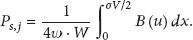
Increase of Sensing Range Temporarily. This task is executed when abrupt faults occur and reduce significantly the probability of sensing coverage. This task implements a 2-step process. In the first step, the probability of coverage is recomputed and compared to a prespecified threshold. The second step takes place when the computed probability is lower than the threshold. In that case the sensors in the vicinity of the faulty node are commanded to increase temporarily their so that the new probability becomes higher than the threshold.

To show how the coverage is recomputed we consider the expression demonstrated in Theorem 3, where we assume only one faulty sensor. We then locate the terms involving the faulty sensor. We recompute them taking into consideration the remaining involved sensors. Then, we reinsert the modified terms to get the final result. The recomputation can be seen through Figure 5, which shows that the area close to the faulty sensor should be deleted in the computation of $P_{s,j}$ , assuming that the sensor landing close to $p_j$ is faulty.

Figure 5

Coverage probability-related areas.

This technique, however, adds complexity to the coverage control, introduces some irregularities to mathematical model controlling the deployment, and may impact the lifetime of the wireless sensor network since the unbalanced distribution of ranges often causes the problem of energy hole, which may induce energy exhaustion of the sensor nodes in the hole region faster than the nodes in other regions [17, 18]. On the other hand, one can agree that the replacement strategy along with a good balance between the time needed to replace failing sensors and the horizon of prediction would compensate such a possible reduction.

7. Simulation

In this section we show the performance of our system by discussing the variation of the radio and sensing coverage probability, in a first step, and by discussing the impact of the replacement strategy, in a second step.

7.1. Radio and Sensing Range Modeling and Simulation

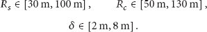
With no loss of generality, we only consider a monitored domain reduced to a thick strip, as depicted by Figure 6. The strip is overlapped by three zones (or squares) where three sensors can land after they are dropped from air. A sensor is assumed to land on discrete positions (separated by δ meters). The parameters $R_s$ , $R_c$ , and δ are assumed to take their values in the following, respectively:

$$\begin{array}{cc}& R_s\in \left[\mathrm{30}\hspace{0.17em}\text{m},\mathrm{100}\hspace{0.17em}\text{m}\right],\hspace{1em}\hspace{1em}{R}_c\in \left[\mathrm{50}\hspace{0.17em}\text{m},\mathrm{130}\hspace{0.17em}\text{m}\right],\\ \delta \in \left[\mathrm{2}\hspace{0.17em}\text{m},\mathrm{8}\hspace{0.17em}\text{m}\right].\end{array}$$

(27)

In addition, we assume that $W=\mathrm{12,5}$  m and the distance between two successive square centers is equal to 70 m. In particular, when $\delta =4$ , then 196 discrete positions can distinguished in the strip. Each sensor can land on one of 56 possible positions.

Figure 6

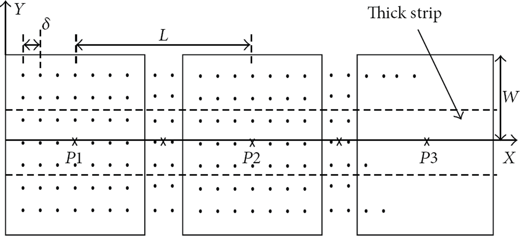
Simulation model.

The simulation is performed as follows: each sensor is dropped randomly on the discrete positions in the related square. The probabilities of sensing and radio coverage are then computed. The drop operation is repeated multiple times and the average probabilities are computed. The resulting values of the mean values are plotted by varying $R_s$ , $R_c$ , and δ. The width of the thick line on which the sensing coverage is obtained is also integrated to analyze its effects on the collected results. In addition, the collected results are compared to those provided by a full random dropping scheme of the three sensors in the strip.

Figure 7 shows the variation of the probability of radio connectivity for different values of $R_c$ , for a fixed value of the discretization step ( $\delta =2\hspace{0.17em}\text{m}$ ). One can notice in this figure that Front-Sense scheme performs better than the full random scheme when $R_c$ becomes higher than $L-W$ and that the full scheme performs better when $R_c$ is smaller. The average increase observed in this figure is higher than 16%. This feature can be explained by the fact that when $R_c$ increases, more space is covered by radio range of the sensor and more opportunity is given to connectivity, when the sensor is assigned to a square.

Figure 7

Probability of connection versus $R_c$ and δ.

In addition, this shows that when $R_c$ is higher than $2W$ , the connectivity is almost guaranteed. Moreover, when $R_c$ is lower than $L-W$ Front-Sense scheme performs lower than the traditional random strategy, since it confines the sensor in smaller set of discrete positions.

Figure 8 depicts the variation of the probability of radio coverage, with respect to the varying communication range $R_c$ , for different values of the intersquare distance $L-2W$ . One can deduce from this figure that Front-Sense scheme performance decreases when $L-2W$ increases and that it increases when $R_c$ increases. It approaches 1 when $R_c$ is higher than $L+2W$ . This feature can be explained by the fact that when $R_c$ increases, more space can be sensed in the three squares. In addition, when the distance between blocks increases, the number of positions where the sensors cannot deploy on becomes important, the distance between the positions of two neighboring sensors increases, and the connectivity is reduced.

Figure 8

Variation of probability of connectivity with respect to $R_c$ .

Figure 9 depicts the variation of the probability of sensing coverage for different values of $R_s$ . Different values of the thick strip width are considered. In particular, one can notice that the probability of sensing coverage gets higher when the strip is reduced to a line $(W=0)$ . It naturally increases with the growth of $R_s$ , since more space in the strip can be covered by the disk located on the sensors. It decreases when the width increases, since one can prove that the points on the main axis of the strip are the most covered by the sensors. In addition, the probability decrease can be more significant once the intersquare distance is high.

Figure 9

Probability of sensing coverage versus $R_s$ and δ.

Let us notice, finally, that the effect of the discretization step δ variations on the probability values in the simulation is not significant when δ is sufficiently small.

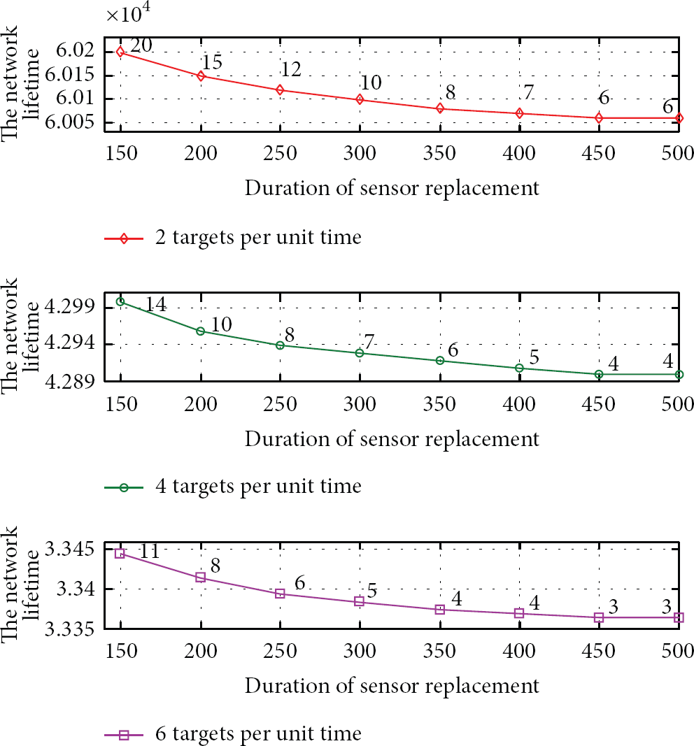
7.2. Impact on Network Lifetime

Let us now evaluate the effect of the sensors’ replacement strategy, proposed in Section 6.2, on the network lifetime and assume that the domain to monitor is a thick strip, containing two lines of sensor drawn along the length of strip. We assume that the lines are 3 Km long and that 30 sensors are deployed on each line uniformly (so that they form squares of side 100 m). Every second square of sensors is assumed to contain in its center a DRN to which the sensors of the square report. Thus, one can see that the points of the two lines are fully covered by the sensors.

While the two definitions of lifetime, discussed in Section 6.2, apply to WSN-based monitoring systems in general, we believe that these definitions do not apply to WSN-based border surveillance systems where the objective of surveillance is not only to locate the individuals crossing the border but also to track them until crossing completion. For this, we provide a third definition that considers the time of failure of the first set of sensors allowing the crossing of an intruder without being detected. Applied to our simulation model, this definition considers the time where the first pair of sensors occurring on different lines and facing each other fail (or get out of energy). Figure 10 depicts the variation of the network lifetime.

Figure 10

Effect of replacement on network lifetime.

To simulate the impact of the replacement strategy on sensors’ lifetime, we assumed the following two issues.

• (1)

Lifetime modeling: when the sensor battery is fully charged, the sensor can send a maximum of 1000 packets to report detected events. Each sensor cannot send more than one packet per unit of time.

(2)

Activity measuring: when not sending a message, the sensor performs normal functioning and consumes little energy. Normal activity during one time unit is assumed to be equal to 1/100 of the required energy to send a message reporting on crossing event.

During simulation two parameters have been varied to assess the impact.

• (3)

The replacement time: this is the time needed to deploy a sensor showing that it is getting out of energy. We varied the values taken by this parameter in the interval $[\mathrm{150,500}]$ , assuming that 100 s corresponds to the horizon of energy shortage. This means that when the remaining energy of a sensor reaches 1/10 of its initial value, a request is sent to replace the sensor.

(4)

The number of targets crossing the monitored area: we considered three rates of targets attempting to cross the monitored area (from one side to the other). They are, respectively, equal to 2, 4, and 6 attempts per 10 time units.

We conducted simulations to measure the network lifetime and the number of replaced sensors to assess the effect of replacement strategy. The results of these simulations are represented in Figure 10.

Let us first notice that if the time to replace a sensor is lower than the time of shortage prediction, the simulation results show that the sensors are all the time replaced. That is why the plotted results start for replacement duration higher than 100 s. Two main observations can be made from the figure.

• (1)

When the replacement time grows from 150 s to 500 s, the network lifetime decreases and the number of replaced sensors becomes smaller. In particular, the number of replaced sensors reaches 40% in the case where one attempt is performed every 10 time slots and the time to replace is 150 s. Indeed, when the time to replace increases, the probability of the sensor requesting replacement goes down before it is replaced gets higher.

(2)

When more crossing attempts are performed per unit of time, the network lifetime gets smaller, for given value of the replacement time. In fact, when more attempts are performed, more sensors will report and more requests for replacement will be generated and the probability that a request is not answered will get more important.

Let us finally notice that if the number of sensing lines in the monitored area increases, then one can be convinced that the lifetime of the network will increase. This feature comes from the fact that more sensors (belonging to different lines) would go to energy shortage before an undetected path occurs.

8. Conclusion

This paper presents a sensor controlled random deployment scheme to monitor bounded 2-dimensional areas while providing mathematical formulations to control the sensor and radio coverage quality it allows. In addition, techniques to detect and repair sensor failures are added to provide system robustness for a large set of WSN-based applications and increase network lifetime. In particular, expressions are set up to define the probability of total coverage when the environment characteristics are varying while taking into consideration real deployment parameters. The cases of two applications, the border surveillance and the wildfire sensing, are considered in some details to show that the approach is generic and that strategies can be conducted and assessed.