Sage Journals: Discover world-class research

Abstract

An integrodifferential equation which describes the charged particle motion for certain configurations of oscillating magnetic fields is considered. The local polynomial regression method (LPR) is used to solve this equation. The reliability of this method and the reduction in the size of computational domain give this method a wider applicability. Several representative examples are given to reconfirm the efficiency of these algorithms. The results of applying this theory to the integro-differential equation with time-periodic coefficients reveal that LPR method possesses very high accuracy, adaptability, and efficiency.

1. Introduction

Most scientific problems in engineering are inherently nonlinear. Except a few number of them, majority of nonlinear problems such as complex integro-differential equation do not have analytical solution. Therefore, these nonlinear equations should be solved using some other methods. Some mathematical methods have been employed to solve different physical differential equations, such as Homotopy perturbation technique by authors [1 –4], Homotopy analysis method given by Dehghan and Shakeri [5], time periodic coefficients by Machado and Tsuchida [6], hysteretic damping used by Chen and You [7], rapidly vanishing convolution kernels by authors [8], Adomian decomposition method by Biazar et al. [9] and Biazar [10], operational tau approximation by Dehcheshmeh et al. [11], Modified Homotopy Perturbation Method by authors [12], the Tau approximation for the delayed Burgers equation by Khaksar Haghani et al. [13], a modified variable separated ordinary differential equation method solving mKdV sinh-Gordon equation by Xie [14], the projective Riccati equation expansion method and variable separation solutions for the nonlinear physical differential equation in physics by Ma [15], and Lagrange-Noether method for solving second-order differential equations by Hui-Bin and Run-Heng [16]. They are all proved to have efficiency and utility widely. Recently, H. Caglar and N. Caglar [17] have used local polynomial regression (LPR) method for the numerical solution of linear and nonlinear Fredholm and Volterra integral equations [17]. Moreover, they manage to solve fifth-order boundary value problems by using LPR method [18]. Numerical results demonstrate that local polynomial fitting method is more accurate, simple, and efficient. In this study, we consider (1) with time-periodic coefficients:

\frac{d^{2} y}{d t^{2}} = - a (t) y (t) + b (t) \int_{0}^{t} \cos (w_{p} s) y (s) d s + g (t),

(1)

where a(t), b(t), and g(t) are given periodic functions of time that may be easily found in the charged particle dynamics for some field configurations. Here, we assume and consider the following initial conditions:

y (0) = α, y^{'} (0) = β .

(2)

The destination of this paper is to use local polynomial regression method for solving integro-differential equations arising in oscillating magnetic fields.

2. Local Polynomial Regression Method

Local polynomial regression technique was first proposed by Hui-Bin and Run-Heng [16] and H. Caglar and N. Caglar [17, 18]. And, this method was also mentioned and used by Su et al. [19 –23]. Recently, H. Caglar and N. Caglar [17, 18] firstly took advantage of local polynomial regression method to try to solve the numerical solution of linear and nonlinear Fredholm and Volterra integral equations successfully and evaluated the efficiency and convenience of the method. Meanwhile, they managed to resolve fifth-order boundary value problems by using local polynomial regression method [18] which also showed the efficiency of this technique. Moreover, by comparing with some methods, for an instance, B-spline method, LPR displayed more accuracy. In order to describe the basic ideas of the LPR, firstly, we introduce the mathematical thoughts of local polynomial regression. This idea was mentioned in detail in [19 –22, 24 –26]. Since the form of regression function is not specified, the data points with long distance from t₀ provide little information to y(t₀). Therefore, we can only use the local data points around t₀. Supposing that y(t) has p + 1 derivative at t₀, by the Taylor expansion, for point t, located in the neighborhood of this point t₀, we can use the p-order multivariate polynomials to locally approximate y(t) and the surrounding local point of t₀; we model y(t) as

y (t) \approx \sum_{j = 0}^{p} ‍ β_{j} {(t - t_{0})}^{j},

(3)

where parameter β_j depends on t₀, so called local parameter. Obviously, the local parameter β_j = y^(j)(t₀)/j! fits the local model with local data and it can be minimized as

\sum_{i = 1}^{n} ‍ {[Y_{i} - \sum_{j = 0}^{p} ‍ β_{j} {(t_{i} - t_{0})}^{j}]}^{2} K (\frac{t_{i} - t_{0}}{h}),

(4)

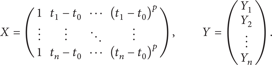
where h controls the size of the bandwidth of local area. Using matrix notation to represent the local polynomial regression is more convenient. Below is the design matrix corresponding to (3) with t and Y:

X = (\begin{pmatrix} 1 & t_{1} - t_{0} & \dots & {(t_{1} - t_{0})}^{p} \\ ⋮ & ⋮ & ⋱ & ⋮ \\ 1 & t_{n} - t_{0} & \dots & {(t_{n} - t_{0})}^{p} \end{pmatrix}), Y = (\begin{pmatrix} Y_{1} \\ Y_{2} \\ ⋮ \\ Y_{n} \end{pmatrix}) .

(5)

The weighted least squares problem (3) can be written as

\min {(Y - X β)}^{T} W (Y - X β) .

(6)

Here,

W = diag (K_{h} (t_{1} - t_{0}), \dots, K_{h} (t_{n} - t_{0})),

(7)

so the solution vector is

β = {(X^{T} W X)}^{- 1} X^{T} W Y .

(8)

Furthermore, we can get the estimation ŷ(t₀):

\hat{y} (t_{0}) = E_{1} {(X^{T} W X)}^{- 1} X^{T} W Y,

(9)

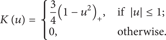
where E₁ is a column vector (the same size of β) with the first element equal to 1 and the rest equal to zero; that is, E₁ = (1, 0,…, 0)_1×(p+1). The selection of K does not influence the results much. We selected the quartic kernel as follows:

K (u) = {\begin{cases} \frac{3}{4} {(1 - u^{2})}_{+}, & if | u | \leq 1; \\ 0, & otherwise . \end{cases}

(10)

3. Parameters Selections

To implement the local polynomial regression and estimator, we need to choose the order p, the kernel K, and the bandwidth h. These parameters are of course related to each other.

First of all, the choice of the bandwidth parameter h is considered, which plays a rather crucial role. A too large bandwidth underparametrizes the regression function [18, 24], causing a large modeling bias, while a too small bandwidth overparametrizes the unknown function and results in noisy estimates. The basic idea is to find a bandwidth h that minimizes the estimated mean integrated square error (MISE):

h_{opt} = \arg \min_{h} \int {{(Bias (\hat{m} (t) ∣ T))}^{2} + Var (\hat{m} (t) ∣ T)} d t,

(11)

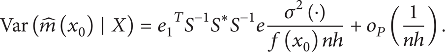
where T = (T₁,…, T_p). We give the asymptotic bias and the asymptotic variance regression function m(x). Assume that f(x₀) > 0 and that f(·), m^{p + 1}(·), and σ²(·) are continuous in a neighborhood of x₀. Further, assume that h → 0 and nh → ∞. Then the asymptotic conditional variance of $\hat{m} (x_{0})$ is given by

Var (\hat{m} (x_{0}) ∣ X) = {e_{1}}^{T} S^{- 1} S^{*} S^{- 1} e \frac{σ^{2} (\cdot)}{f (x_{0}) n h} + o_{P} (\frac{1}{n h}) .

(12)

The asymptotic conditional bias for p − v odd is given by

Bias {\hat{m} (x_{0}) ∣ X} = {e_{1}}^{T} S^{- 1} c_{p} \frac{1}{(p + 1)!} m {(x_{0})}^{p + 1} h^{p + 1} + o_{P} (h^{p + 1}) .

(13)

The asymptotic conditional bias for p − v even is given by

\begin{matrix} Bias {\hat{m} (x_{0}) ∣ X} \\ = e_{1} S^{- 1} {\tilde{c}}_{p} \frac{1}{(p + 2)!} \\ \times {m^{p + 2} (x_{0}) + (p + 2) m {(x_{0})}^{p + 1} \frac{f^{'} (x_{0})}{f (x_{0})}} h^{p + 2} \\ + o_{P} (h^{p + 2}) \end{matrix}

(14)

provided that f′(·) and m^{p + 2}(·) are continuous in a neighborhood of x₀ and nh³ → ∞, where

\begin{matrix} S = {(μ_{j + l})}_{0 \leq j, l \leq p}, S^{*} = {(v_{j + l})}_{0 \leq j, l \leq p}, \\ c_{p} = {(μ_{p + 1}, \dots, μ_{2 p + 1})}^{T}, {\tilde{c}}_{p} = {(μ_{p + 2}, \dots, μ_{2 p + 2})}^{T}, \\ e_{1} = {(1,0, 0, \dots, 0)}^{T} . \end{matrix}

(15)

The moments of K and K² are denoted, respectively, by

μ_{j} = \int ‍ u^{j} K (u) d u, v_{j} = \int ‍ u^{j} K^{2} (u) d u,

(16)

h_{opt} = c_{ν, p} (K) {[\frac{\int ‍ (σ^{2} (t) / f (t))}{\int {m^{(p + 1)} (t) d t}}]}^{1 / (2 p + 3)} n^{- 1 / (2 p + 3)},

(17)

(Proof see Rupper and Wand [27]), where c_{ν, p}(K) is a constant which relates of the kernel function and the order of the local polynomial f(t) is the density function of m(·). However, this ideal bandwidth is not directly usable since it depends on unknown functions.

Another issue in local polynomial fitting is the choice of the order of the polynomial. Since the modeling bias is primarily controlled by the bandwidth, the issue is less crucial. For a given bandwidth h, a large value of p would expectedly reduce the modeling bias, but would cause a large variance and a considerable computational cost. It is shown in [25] that there is a general pattern of increasing variability; for estimate m^(ν)(t₀), there is no increase in variability when passing from an even (i.e., p − ν even) p = ν + 2q order fit to an odd p = ν + 2q + 1 order fit, but when passing from an odd p = ν + 2q + 1 order fit to the consecutive even p = ν + 2q + 2, order fit, there is a price to be paid in terms of increased variability. Therefore, even order fits p = ν + 2q are not recommended. Since the bandwidth is used to control the modeling complexity, we recommend the use of lowest odd order; that is, p = ν + 1 or occasionally p = ν + 3.

Another question concerns the choice of the kernel function K. Since the estimation is based on the local regression equation (4), no negative weight K should be used. As shown in [25], the optimal weight function is K(z) = (3/4)(1 − z²)₊, the Epanechnikov kernel, which minimizes the asymptotic mean square error (MSE) of the resulting local polynomial estimators.

4. Solution of the Integrodifferential Equation

In this section, the LPR method for solving (1)–(2) is outlined. Letting (3) be an approximate solution of (1)–(2),

y (t) \approx \sum_{j = 0}^{p} ‍ β_{j} {(t - t_{0})}^{j},

(18)

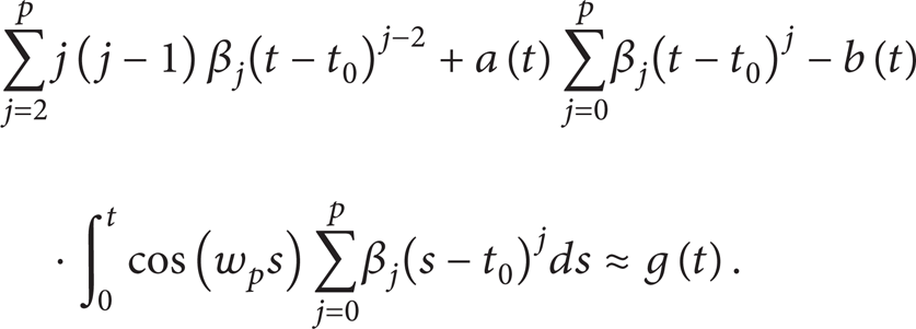
where t₁ = 0 < t₂ < ⋯ < t_n = 1. We can adjust the value of parameter n flexibly, and it is required that the approximate solution (19) satisfies (1)–(2) at the point t = t_i. Therefore, we can transform (1) to (19):

\frac{d^{2} y}{d t^{2}} + a (t) y (t) - b (t) \int_{0}^{t} ‍ \cos (w_{p} s) y (s) d s = g (t) .

(19)

Putting (18) in (19), then we can get the following:

\begin{matrix} \sum_{j = 2}^{p} ‍ j (j - 1) β_{j} {(t - t_{0})}^{j - 2} + a (t) \sum_{j = 0}^{p} ‍ β_{j} {(t - t_{0})}^{j} - b (t) \\ \cdot \int_{0}^{t} ‍ \cos (w_{p} s) \sum_{j = 0}^{p} ‍ β_{j} {(s - t_{0})}^{j} d s \approx g (t) . \end{matrix}

(20)

In order to satisfy unique solution theorem of integral-differential equation, we should take initial conditions (2) into account. Consequently, putting (18) to initial conditions (2), then we can acquire the approximate expression (21) as follows:

\sum_{j = 0}^{p} ‍ β_{j} {(t - t_{0})}^{j} \approx α, \sum_{j = 1}^{p} ‍ j β_{j} {(t - t_{0})}^{j - 1} \approx β,

(21)

where t₁ = t₂ = 0. Consequently, we can deduce the minimization function of (1)–(2) from (4); the minimization function can be written as

\begin{matrix} {[y (0) - \sum_{j = 0}^{p} ‍ β_{j} {(t_{1} - t_{0})}^{j}]}^{2} \cdot K_{h} (t_{1} - t_{0}) \\ + {[y^{'} (0) - \sum_{j = 0}^{p} ‍ β_{j} {(t_{2} - t_{0})}^{j}]}^{2} \cdot K_{h} (t_{2} - t_{0}) \\ + \sum_{i = 3}^{p} ‍ {g (t_{i}) - [\sum_{j = 2}^{p} ‍ j (j - 1) β_{j} {(t_{i} - t_{0})}^{j - 2} \\ + a (t) \cdot \sum_{j = 0}^{p} ‍ β_{j} {(t_{i} - t_{0})}^{j} - b (t_{i}) \\ \cdot \int_{0}^{t_{i}} ‍ \cos (w_{p} s) \sum_{j = 0}^{p} ‍ β_{j} {(s - t_{0})}^{j} d s]} \\ \cdot K_{h} (t_{i} - t_{0}), \end{matrix}

(22)

t₁ = 0 where and t₂ = 0. Combining (20), (21) with (22), we can acquire the system which can be expressed as

\begin{matrix} i = 1, \\ a_{1, j} = {(t_{1} - t_{0})}^{j}, j = 0, \dots, p, y (1) = α, t_{1} = 0; \\ i = 2, \\ a_{2, j} = j {(t_{2} - t_{0})}^{j - 1}, j = 1, \dots, p, y (2) = β, t_{2} = 0; \\ i = 3, \dots, n, \\ a_{3, j} = j (j - 1) {(t_{i} - t_{0})}^{j - 2}, j = 2, \dots, p, \\ b_{i, j} = a (t_{i}) {(t_{i} - t_{0})}^{j}, j = 0, \dots, p, \\ c_{i, j} = b (t_{i}) \int_{0}^{t_{i}} ‍ \cos (w_{p} s) {(s - t_{0})}^{j} d t, j = 1, \dots, p, \\ y (i) = g (t_{i}); \end{matrix}

(23)

then, the matrix form (5) can be written as follows by using (23)–(24):

X = [\begin{bmatrix} a_{10} & a_{11} & \dots & \dots & \dots & a_{1 p} \\ a_{20} & a_{21} & \dots & \dots & \dots & a_{2 p} \\ b_{30} + c_{30} & b_{31} + c_{31} & d_{31} & \dots & \dots & d_{3 p} \\ b_{40} + c_{40} & b_{41} + c_{41} & d_{41} & \dots & \dots & d_{4 p} \\ ⋮ & ⋮ & ⋮ & ⋮ & ⋮ & ⋮ \\ b_{n - 1,0} + c_{n - 1,0} & b_{n - 1,1} + c_{n - 1,1} & d_{n - 1} & \dots & \dots & \dots \\ b_{n, 0} + c_{n, 0} & b_{n, 1} + c_{n, 1} & d_{n} & \dots & \dots & d_{n, p} \end{bmatrix}],

(24)

Y = [\begin{bmatrix} y (1) \\ y (2) \\ ⋮ \\ y (n) \end{bmatrix}] .

(25)

where d₃ = a₃₂ + b₃₂ + c₃₂, d₄ = a₄₂ + b₄₂ + c₄₂, d_{n − 1} = a_n−1,2 + b_n−1,2 + c_n−1,2, d_n = a_n2 + b_n2 + c_n2, d_3p = a_3p + b_3p + c_3p, d_4p = a_4p + b_4p + c_4p, d_np = a_np + b_np + c_np,

\begin{matrix} w_{p} = 2, \\ a (t) = \cos (t), b (t) = \sin (\frac{t}{2}), \\ g (t) = \cos (t) - t \sin (t) + \cos (t) (t \sin (t) + \cos (t)) - \sin (\frac{t}{2}) (\frac{2}{9} \sin (3 t) - \frac{t}{6} \cos (3 t) + \frac{t}{2} \cos (t)), \\ α = 1, β = 0, \end{matrix}

(26)

Putting (24)–(25) to (9), then estimated set of coefficients β_i can be obtained by solving matrix system solution; therefore, approximate-value ŷ(t₀) at point t₀ can be obtained.

5. Illustrative Tests

In this section, to illustrate the description above and to show the efficiency of the mentioned method for solving (1)–(2), we include some examples with known analytical solutions.

Test 1. Considering (1) with

y^{′′} (t) = - \cos (t) y (t) + \sin (\frac{t}{2}) \int_{0}^{t} ‍ \cos (2 s) y (s) d s + g (t),

(27)

y(t) = t sin(t) + cos (t) is the exact solution of this equation.

Then we have

y (0) = 1, y^{'} (0) = 0 .

(28)

To apply the local polynomial regression method to this equation, based on (9), (24), and (25), we calculate the numerical results and absolute errors at point t = 0.0, 0.2, 0.4, 0.6, 0.8, 1.0 by setting up different parameters p, h, and n. Numerical results obtained by these approximations are summarized in Table 1. Figure 1 also reveals the results detailed and explicitly.

Table 1:

The numerical results and absolute errors at point t = 0.0, 0.2, 0.4, 0.6, 0.8, 1.0 given different parameters p, h, and n, Test 1, where LPR(a, b) stands for LPR(h, n).

t	p	LPR(0.085, 30)	LPR(0.07, 30)	LPR(0.055, 30)

0.0	5	4.72313 × 10⁻⁵	8.07321 × 10⁻⁷	5.01625 × 10⁻⁸
0.2	5	2.11645 × 10⁻⁴	1.10985 × 10⁻⁵	1.00321 × 10⁻⁶
0.4	5	3.05049 × 10⁻⁴	4.28762 × 10⁻⁵	2.46247 × 10⁻⁶
0.6	6	3.63704 × 10⁻⁴	4.80046 × 10⁻⁵	2.91992 × 10⁻⁶
0.8	6	1.92052 × 10⁻⁴	3.93021 × 10⁻⁵	1.83003 × 10⁻⁶
1.0	6	6.59121 × 10⁻⁶	1.54302 × 10⁻⁶	3.23692 × 10⁻⁸

t	p	LPR(0.075, 50)	LPR(0.055, 50)	LPR(0.045, 50)

0.0	7	3.52451 × 10⁻⁸	8.8383 × 10⁻⁹	2.56 × 10⁻¹¹
0.2	7	8.31715 × 10⁻⁸	1.07079 × 10⁻⁸	1.89021 × 10⁻¹⁰
0.4	7	2.14093 × 10⁻⁷	4.81965 × 10⁻⁸	3.69002 × 10⁻¹⁰
0.6	7	2.62107 × 10⁻⁷	3.43041 × 10⁻⁸	3.07524 × 10⁻¹⁰
0.8	8	1.05032 × 10⁻⁸	2.26808 × 10⁻⁸	8.52800 × 10⁻¹¹
1.0	8	6.42234 × 10⁻⁹	8.84534 × 10⁻⁹	6.35639 × 10⁻¹¹

Considering Table 1, we solve the example with n = 30, 50 by choosing p = 5, 6, 7, 8 given various values of parameters h presented in Table 1. The absolute errors in the solutions are computed. Given n = 30, p = 5, 6, it can be seen that the magnitude of absolute errors is between 10 to the power of −4 and 10 to the power of −8. Nevertheless, by setting up n = 50, p = 7, 8, it is obvious that the magnitude of absolute errors is between 10 to the power of −7 and 10 to the power of −11. We conclude that absolute errors decrease with the increase of the value of n and the value of order p has no much influence on absolute errors. Considering only parameter h, specifically, absolute errors get up to minimum for p = 5, 6, n = 30 when h = 0.055, for p = 7, 8, n = 50 when h = 0.045. We can find that the optimal bandwidth h locates in district [0.045, 0.055] by using LPR for n = 30, 50.

Figure 1:

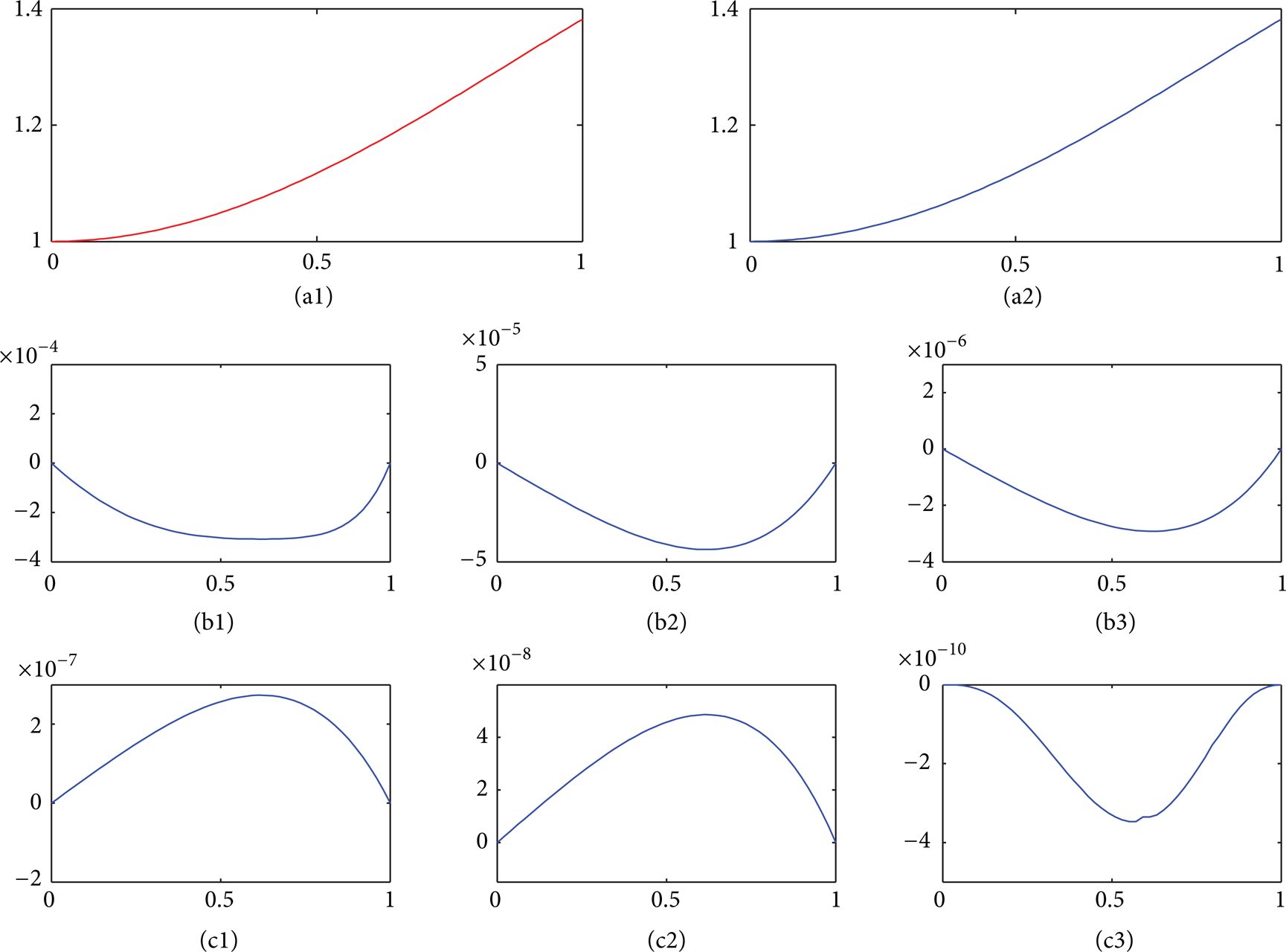
(a1) The exact solution; (a2) the LPR solution for n = 50, p = 7, h = 0.085: the error function for (b1) n = 30, p = 5, h = 0.085: (b2) n = 30, p = 5, h = 0.07: (b3) n = 30, p = 6, h = 0.055: (c1) n = 50, p = 7, h = 0.075: (c2) n = 50, p = 8, h = 0.055: (c3) n = 50, p = 8, h = 0.045 in Test 1.

Test 2. As for the second example, consider (1) with

\begin{matrix} w_{p} = 1, \\ a (t) = - \sin (t), b (t) = \sin (t), \\ g (t) = \frac{1}{9} e^{- t / 3} - \sin (t) (e^{- t / 3} + t) - \sin (t) (- \frac{3}{10} \cos (t) e^{- t / 3} + \frac{9}{10} e^{- t / 3} \sin (t) + \cos (t) + t \sin (t) - \frac{7}{10}), \\ α = 1, β = \frac{2}{3} . \end{matrix}

(29)

y(t) = e^−t/3 + t is the exact solution of this problem. Then we have

\begin{matrix} y^{′′} (t) = - \sin (t) y (t) + g (t) + \sin (t) \int_{0}^{x} ‍ \cos (s) y (s) d s, \\ y (0) = 1, y^{'} (0) = \frac{2}{3}, \end{matrix}

(30)

similar to Test 1. We take advantage of the local polynomial regression method to solve this equation, based on (9), (24) and (25) which we deduced above. Then we can calculate the numerical results and absolute errors at point t = 0.0, 0.2, 0.4, 0.6, 0.8, 1.0 by given different parameters p, h, and n. Numerical results are concluded in Table 2 and Figure 2.

Considering Table 2, we solve the example with n = 30, 50 by choosing p = 5, 6, 8, 9 given various values of parameters h presented in Table 1. The absolute errors in the solutions are computed. Given n = 30, p = 5, 6, it can be seen that the magnitude of absolute errors is between 10 to the power of −4 and 10 to the power of −8. Nevertheless, by setting up n = 50, p = 8, 9, it is obvious that the magnitude of absolute errors is between 10 to the power of −9 and 10 to the power of −13. We conclude that absolute errors decrease with the increase of the value of n and the value of order p has no much influence on absolute errors. Again, considering parameter h, specifically, absolute errors get up to minimum for p = 5, 6, n = 30 when h = 0.065, for p = 8, 9, n = 50 when h = 0.045. We can find that the optimal bandwidth h locates approximately in district [0.045, 0.065] by using LPR for n = 30, 50.

Table 2:

The numerical results and absolute errors at point t = 0.0, 0.2, 0.4, 0.6, 0.8, 1.0 by setting up different parameters p, h, and n, Test 2, where LPR(a, b) stands for LPR(h, n).

t	p	LPR(0.085, 30)	LPR(0.07, 30)	LPR(0.065, 30)

0.0	5	5.58724 × 10⁻⁵	6.07321 × 10⁻⁷	4.01625 × 10⁻⁸
0.2	5	4.56321 × 10⁻⁵	3.54025 × 10⁻⁶	1.34023 × 10⁻⁷
0.4	6	3.03420 × 10⁻⁴	2.27608 × 10⁻⁶	1.50252 × 10⁻⁷
0.6	6	3.60352 × 10⁻⁴	2.73056 × 10⁻⁶	1.63534 × 10⁻⁷
0.8	6	2.13394 × 10⁻⁴	6.94352 × 10⁻⁶	2.83021 × 10⁻⁷
1.0	6	4.07545 × 10⁻⁵	2.14061 × 10⁻⁷	5.23602 × 10⁻⁸

t	p	LPR(0.055, 50)	LPR(0.045, 50)	LPR(0.045, 70)

0.0	8	6.59022 × 10⁻¹⁰	5.52012 × 10⁻¹¹	2.17601 × 10⁻¹²
0.2	8	5.05323 × 10⁻¹⁰	2.23609 × 10⁻¹¹	1.66721 × 10⁻¹²
0.4	8	1.35113 × 10⁻⁹	3.59231 × 10⁻¹⁰	2.30217 × 10⁻¹²
0.6	9	1.56323 × 10⁻⁹	3.34001 × 10⁻¹⁰	3.72184 × 10⁻¹²
0.8	9	6.50112 × 10⁻¹⁰	8.17318 × 10⁻¹¹	4.41052 × 10⁻¹³
1.0	9	4.63511 × 10⁻¹⁰	6.09124 × 10⁻¹¹	6.39016 × 10⁻¹³

Figure 2:

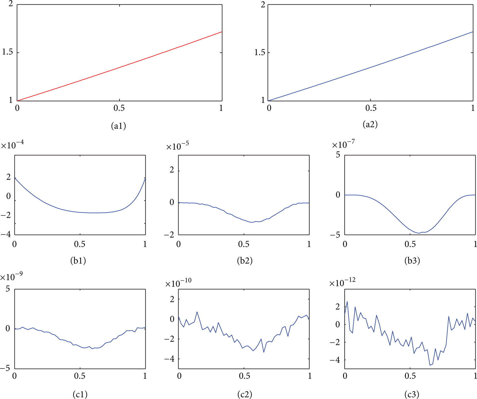
(a1) The exact solution; (a2) the LPR solution for n = 50, p = 5, h = 0.07: the error function for (b1) n = 30, p = 5, h = 0.085: (b2) n = 30, p = 6, h = 0.07: (b3) n = 30, p = 6, h = 0.065: (c1) n = 50, p = 8, h = 0.055: (c2) n = 50, p = 9, h = 0.045: (c3) n = 70, p = 9, h = 0.045 in Test 2.

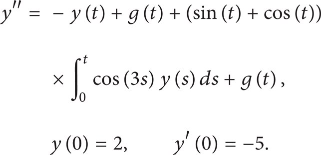
Test 3. In this example, consider (1) with

\begin{matrix} w_{p} = 3, \\ a (t) = 1, b (t) = \sin (t) + \cos (t), \\ g (t) = - t^{3} + t^{2} - 11 t + 4 - (\sin (t) + \cos (t)) \times (- \frac{t^{3}}{3} \sin (3 t) - \frac{t^{2}}{3} \cos (3 t) - \frac{13}{27} \cos (3 t) - \frac{13}{9} t \sin (3 t) + \frac{t^{2}}{3} \sin (3 t) + \frac{16}{27} \sin (3 t) + \frac{2}{9} t \cos (3 t) + \frac{13}{27}) . \end{matrix}

(31)

α = 1, β = 0, y(t) = − t³ + t² − 5t + 2 is the exact solution of this equation. Consequently, we have

\begin{matrix} y^{′′} = - y (t) + g (t) + (\sin (t) + \cos (t)) \times \int_{0}^{t} ‍ \cos (3 s) y (s) d s + g (t), \\ y (0) = 2, y^{'} (0) = - 5 . \end{matrix}

(32)

Similar to Tests 1 and 2, appling the local polynomial regression method to this equation, based on the (9), (24), and (25), we calculate the numerical results and absolute errors at point t = 0.0, 0.1, 0.3, 0.5, 0.7, 0.9, 1.0 by setting up different parameters p, h, and n. Numerical results obtained by these approximations are also explained in Table 3. Figure 3 provides exact solution, LPR solution, and different error functions given by kinds of parameters.

Considering Table 3, we resolve example 3 with n = 30, 50, 70 by choosing p = 7, 8, 9 given various values of parameters h presented in Table 1. The absolute errors in the solutions are computed. Given n = 30, p = 7, 8, it can be seen that the magnitude of absolute errors is between 10 to the power of −4 and 10 to the power of −8. By setting up n = 50, p = 8, 9, it is obvious that the magnitude of absolute errors is between 10 to the power of −7 and 10 to the power of −11. Nevertheless, By setting up n = 70, p = 8, 9, it is obvious that the magnitude of absolute errors is between 10 to the power of −10 and 10 to the power of −13. We conclude that absolute errors decrease with the increase of the value of n and the value of order p has no much influence on absolute errors. Again, considering parameter h, specifically, absolute errors get up to minimum for p = 7, 8, 9, n = 50 when h = 0.045, for p = 8, 9, n = 50 when h = 0.048. We can find that the optimal bandwidth h also locates approximately in district [0.045, 0.05] by using LPR for n = 50, 70.

Table 3:

The numerical results and absolute errors at point t = 0.0, 0.1, 0.3, 0.5, 0.7, 0.9 given different parameters p, h, and n, Test 3, where LPR(a, b) stands for LPR(h, n).

t	p	LPR(0.085, 30)	LPR(0.07, 50)	LPR(0.055, 50)

0.0	7	3.32702 × 10⁻⁵	5.22185 × 10⁻⁷	6.03139 × 10⁻⁹
0.1	7	1.01732 × 10⁻⁴	3.26213 × 10⁻⁸	2.51244 × 10⁻⁷
0.3	7	1.62303 × 10⁻⁴	1.21808 × 10⁻⁷	5.27411 × 10⁻⁹
0.5	8	1.86343 × 10⁻⁴	1.60356 × 10⁻⁷	1.42331 × 10⁻⁸
0.7	8	4.30659 × 10⁻⁵	5.30215 × 10⁻⁷	2.23021 × 10⁻⁸
0.9	8	3.58816 × 10⁻⁵	2.45293 × 10⁻⁸	5.14652 × 10⁻⁹

t	p	LPR(0.045, 50)	LPR(0.056, 70)	LPR(0.048, 70)

0.0	8	3.51246 × 10⁻¹¹	4.11289 × 10⁻¹²	2.31902 × 10⁻¹²
0.1	8	2.48101 × 10⁻¹⁰	1.37055 × 10⁻¹¹	8.07728 × 10⁻¹³
0.3	9	2.61513 × 10⁻¹⁰	1.59231 × 10⁻¹⁰	2.30217 × 10⁻¹²
0.5	9	1.56323 × 10⁻¹⁰	3.08027 × 10⁻¹⁰	2.69071 × 10⁻¹²
0.7	9	3.50112 × 10⁻¹⁰	2.56023 × 10⁻¹¹	4.42302 × 10⁻¹³
0.9	9	4.63511 × 10⁻⁹	7.53341 × 10⁻¹²	2.31016 × 10⁻¹³

Figure 3:

(a1) The exact solution; (a2) the LPR solution for n = 70, p = 9, h = 0.048: the error function for (b1) n = 30, p = 5, h = 0.085: (b2) n = 30, p = 6, h = 0.055: (b3) n = 50, p = 7, h = 0.055: (c1) n = 50, p = 8, h = 0.04: (c2) n = 70, p = 9, h = 0.056: (c3) n = 70, p = 9, h = 0.048 in Test 3.

6. Conclusions

This paper deals with the numerical solution of an integro-differential equation with time-periodic coefficients which describe the charged particle motion for certain configurations of oscillating magnetic fields by using local polynomial regression method. The kind of technique was tested on three examples and was seen to produce satisfactory results. The reliability of the method and the reduction in the size of computational domain give this method a wider applicability. Furthermore, this technique, in contrast to the traditional methods, does not require a small parameter and the approximations obtained by the proposed method are uniformly valid not only for small parameters but also for very large parameters. The numerical results obtained in this research are indistinguishable due to the fact that this approach justifies its efficiency and presents quite promising results and provides a very high degree of accuracy and efficiency which can be adjused by changing three kinds of parameters p, h, and n without any restrictive assumptions.

Conflict of Interests

The authors declare that they have no possible conflict of interests with any trademark mentioned in the paper.

Footnotes

Acknowledgments

This project was supported by the Natural Science Foundation Project of CQ CSTC of China (Grant no. CSTC2011jjA40033 and Grant no. CSTC2012jjA00037) and was supported by Scientific and Technological Research Program of Chongqing Municipal Education Commission (Grant no. KJ120829).

References

Saberi-Nik

Effati

, and Buzhabad

, “Analytic-approximate solution for an integro-differential equation arising in oscillating magnetic fields using homotopy analysis method,” Iranian Journal of Optimization, vol. 3, no. 10, pp. 518–535, 2010.

J.-H.

, “Homotopy perturbation method: a new nonlinear analytical technique,” Applied Mathematics and Computation, vol. 135, no. 1, pp. 73–79, 2003.

J.-H.

, “The homotopy perturbation method for nonlinear oscillators with discontinuities,” Applied Mathematics and Computation, vol. 151, no. 1, pp. 287–292, 2004.

J.-H.

, “Homotopy perturbation method for solving boundary value problems,” Physics Letters A, vol. 350, no. 1–2, pp. 87–88, 2006.

Dehghan

and Shakeri

, “Solution of an integro-differential equation arising in oscillating magnetic fields using he's homotopy perturbation method,” Progress in Electromagnetics Research, vol. 78, pp. 361–376, 2008.

Machado

J. M.

and Tsuchida

, “Solutions for a class of integro-differential equations with time periodic coefficients,” Applied Mathematics E, vol. 2, pp. 66–71, 2002.

Chen

J. T.

and You

D. W.

, “An integral-differential equation approach for the free vibration of a SDOF system with hysteretic damping,” Advances in Engineering Software, vol. 30, no. 1, pp. 43–48, 1999.

Hoppensteadt

F. C.

Jackiewicz

, and Zubik-Kowal

, “Numerical solution of Volterra integral and integro-differential equations with rapidly vanishing convolution kernels,” BIT Numerical Mathematics, vol. 47, no. 2, pp. 325–350, 2007.

Biazar

Babolian

, and Islam

, “Solution of the system of ordinary differential equations by Adomian decomposition method,” Applied Mathematics and Computation, vol. 147, no. 3, pp. 713–719, 2004.

10.

Biazar

, “Solution of systems of integral-differential equations by Adomian decomposition method,” Applied Mathematics and Computation, vol. 168, no. 2, pp. 1232–1238, 2005.

11.

Dehcheshmeh

S. S.

Vanani

S. K.

, and Hafshejani

J. S.

, “Operational Tau approximation for the Fokker-Planck equation,” Chinese Physics Letters, vol. 29, no. 4, Article ID 045201, 2012.

12.

Yao-Bin

Zhong-Wei

, and Si-Wei

, “Modified homotopy perturbation method for certain strongly nonlinear oscillators,” Chinese Physics Letters, vol. 29, no. 6, Article ID 060502, 2012.

13.

Haghani

F. Khaksar

Vanani

S. Karimi

, and Hafshejani

J. Sedighi

, “Numerical computation of the tau approximation for the delayed burgers equation the tau approximation,” Chinese Physics Letters, vol. 30, no. 2, Article ID 020201, 2013.

14.

Xie

Y.-X.

, “Solving mKdV-sinh-Gordon equation by a modified variable separated ordinary differential equation method,” Chinese Physics B, vol. 18, no. 12, pp. 5123–5132, 2009.

15.

Z.-Y.

, “The projective Riccati equation expansion method and variable separation solutions for the nonlinear physical differential equation in physics,” Chinese Physics, vol. 16, no. 7, pp. 1848–1854, 2007.

16.

Hui-Bin

and Run-Heng

, “Lagrange-Noether method for solving second-order differential equations,” Chinese Physics B, vol. 18, no. 9, pp. 3647–3650, 2009.

17.

Caglar

and Caglar

, “Solution of fifth order boundary value problems by using local polynomial regression,” Applied Mathematics and Computation, vol. 186, no. 2, pp. 952–956, 2007.

18.

Caglar

and Caglar

, “Numerical solution of integral equations by usinglocal polynomial regression,” Journal of Computational Analysis and Applications, vol. 10, no. 2, pp. 187–195, 2008.

19.

L. Y.

and Li

, “Deconvolution of defocused image with multivariate local polynomial regression and iterative wiener filtering in DWT domain,” Mathematical Problems in Engineering, vol. 2010, Article ID 605241, 14 pages, 2010.

20.

L.-Y.

, “Prediction of multivariate chaotic time series with local polynomial fitting,” Computers and Mathematics with Applications, vol. 59, no. 2, pp. 737–744, 2010.

21.

, “Multivariate local polynomial regression with application to Shenzhen component index,” Discrete Dynamics in Nature and Society, vol. 2011, Article ID 930958, 11 pages, 2011.

22.

L. Y.

Zhao

, and Yan

, “Two-stage method based on local polynomial fitting for a linear heteroscedastic regression model and its application in economics,” Discrete Dynamics in Nature and Society, vol. 2012, Article ID 696927, 17 pages, 2012.

23.

L.-Y.

Y.-J.

, and Li

J.-J.

, “Application of local polynomial estimation in suppressing strong chaotic noise,” Chinese Physics B, vol. 21, no. 2, Article ID 020508, 2012.

24.

Fan

and Yao

, Nonlinear Time Series: Nonparametric and Parametric Methods, Springer, New York, NY, USA, 2003.

25.

Fan

and Gijbels

, Local Polynomial Modelling and Its Applications, Chapman Hall, London, UK, 1996.

26.

Fan

and Gijbels

, “Data-driven bandwidth selection in local polynomialfitting: variable bandwidth and spatial adaptation,” Journal of the Royal Statistical Society, vol. 57, pp. 371–394, 1995.

27.

Rupper

and Wand

M. P.

, “Multivariate weighted least squares regression,” Annals of Statistics, vol. 6, pp. 1122–1137, 1994.

Solution of an Integral-Differential Equation Arising in Oscillating Magnetic Fields Using Local Polynomial Regression

Abstract

1. Introduction

2. Local Polynomial Regression Method

3. Parameters Selections

4. Solution of the Integrodifferential Equation

5. Illustrative Tests

6. Conclusions

Conflict of Interests

Footnotes

Acknowledgments

References