Sage Journals: Discover world-class research

Abstract

We consider a system of coupled partial differential equations describing transient fluid flow and heat transfer with variable flow properties. Classical Lie point symmetry analysis of this system resulted in admitted large Lie algebras for some special cases of the arbitrary constants and the source term. Symmetry reductions are performed and as such the system of partial differential equations is reduced to the system of ordinary differential equations. Some reduced ordinary differential equation could be solved exactly with restrictions on the parameters appearing in it. In addition, shooting quadrature is employed to numerically tackle the nonlinear model boundary value problem and pertinent results are presented graphically and discussed quantitatively.

1. Introduction

Transient flow and heat transfer in an incompressible fluid with variable properties play a significant role in engineering and industrial flow processes [1]. For instance, liquid metals having low Prandtl number (because of very large thermal conductivity) are generally used as coolants and have applications in manufacturing processes such as the cooling of the metallic plate and nuclear reactor. Liquid metal has the ability to transport heat even if small temperature difference exists between the surface and fluid. For this reason liquid metal is used as coolant in nuclear reactor to transfer waste heat from the core region. However, it is expected that coolant would never boil and temperature stability must be constantly maintained; hence the pressure is kept at normal level to prevent leak and accidents. In this context, various thermophysical parameters affecting the heat transfer like variable viscosity and thermal conductivity must be studied carefully for proper and optimal performance of engineering system. In addition, the knowledge of flow and heat transfer within a thin liquid film is crucial in understanding the coating process and designing of heat exchangers and chemical processing equipment. This interest stems from many engineering and geophysical applications such as geothermal reservoirs and other applications including wire and fibre coating, food stuff processing, reactor fluidization, transpiration cooling, thermal insulation, enhanced oil recovery, packed bed catalytic reactors, and underground energy transport.

The study of heat transfer and the flow field is necessary for determining the quality of the final products of these processes as explained by Andersson et al. [2]. Tsou et al.[3] presented an analysis of flow and heat transfer over a continuous moving surface. The effect of temperature dependent variable viscosity on laminar flow due to a point sink was studied by Eswara and Bommaih [4]. Several other authors such as those in [5 –7] have established that temperature dependent viscosity has a pronounced effect on the momentum and thermal transport in the boundary layer region. In order to accurately predict the flow and the heat transfer rate it is necessary to take into account the variation of viscosity and thermal conductivity. Meanwhile, the nonlinear nature of the variable viscosity and thermal conductivity functions precludes the exact solution for the governing flow and heat transfer equations. However, with the use of classical symmetry methods, it may be possible to reduce the model equations to tractable form of ODEs which may be solved exactly or numerically (see, e.g., [8 –11]). To the best knowledge of the authors, the combined effects of unsteadiness, power laws variable viscosity, and thermal conductivity on fluid flow and heat transfer over a flat surface with arbitrary heat source have not been reported yet in the literature.

Hence, the main objective of this present study is to analyse and numerically investigate the effects of power laws variable viscosity and thermal conductivity on unsteady boundary layer flow of a viscous incompressible fluid and heat transfer over a flat plate in the presence of variable heat source. This paper is organized as follows; governing equations are derived in Section 2, and in Section 3, we provide a brief theory on Lie point symmetry analysis. Section 4 deals with the similarity reduction of the system of equations modelling transient fluid flow and heat transfer with variable properties. Numerical procedures are discussed in Section 5. In Section 6 we present some results and discussion, and lastly we conclude in Section 7.

2. Governing Equations

Here, we consider the transient flow of an incompressible viscous fluid and heat transfer with external heat source and variable thermophysical properties. The fluid dynamic viscosity and thermal conductivity are assumed to be temperature dependent. The basic one-dimensional equations of momentum and energy balance in original variables are

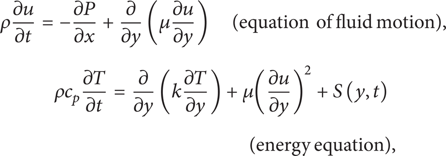
\begin{matrix} ρ \frac{\partial u}{\partial t} = - \frac{\partial P}{\partial x} + \frac{\partial}{\partial y} (μ \frac{\partial u}{\partial y}) (equation of fluid motion), \\ ρ c_{p} \frac{\partial T}{\partial t} = \frac{\partial}{\partial y} (k \frac{\partial T}{\partial y}) + μ {(\frac{\partial u}{\partial y})}^{2} + S (y, t) (energy equation), \end{matrix}

(1)

where ρ is the fluid density, k is thermal conductivity, S(y, t) is the external heat source, μ is the fluid dynamic viscosity, u is the velocity, T is the temperature, P is pressure, t is time, c_p is the specific heat at constant pressure, and (x, y) are the axial and transverse coordinate, respectively. The fluid viscosity and thermal conductivity are assumed to vary as follows:

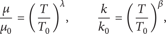
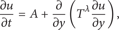
\frac{μ}{μ_{0}} = {(\frac{T}{T_{0}})}^{λ}, \frac{k}{k_{0}} = {(\frac{T}{T_{0}})}^{β},

(2)

where μ₀, T₀, λ, and β are the dynamic viscosity coefficient, fluid initial temperature, thermal conductivity coefficient, variable viscosity exponent, and variable thermal conductivity exponent, respectively. The following dimensionless variables are introduced:

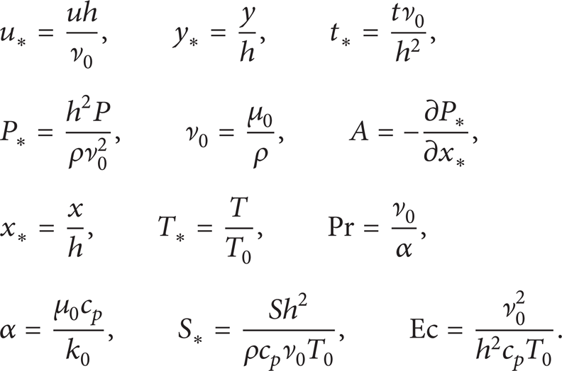
\begin{matrix} u_{*} = \frac{u h}{ν_{0}}, y_{*} = \frac{y}{h}, t_{*} = \frac{t ν_{0}}{h^{2}}, \\ P_{*} = \frac{h^{2} P}{ρ ν_{0}^{2}}, ν_{0} = \frac{μ_{0}}{ρ}, A = - \frac{\partial P_{*}}{\partial x_{*}}, \\ x_{*} = \frac{x}{h}, T_{*} = \frac{T}{T_{0}}, Pr = \frac{ν_{0}}{α}, \\ α = \frac{μ_{0} c_{p}}{k_{0}}, S_{*} = \frac{S h^{2}}{ρ c_{p} ν_{0} T_{0}}, Ec = \frac{ν_{0}^{2}}{h^{2} c_{p} T_{0}} . \end{matrix}

(3)

Neglecting the star for clarity, we obtain the dimensionless system of partial differential equations (PDEs):

\frac{\partial u}{\partial t} = A + \frac{\partial}{\partial y} (T^{λ} \frac{\partial u}{\partial y}),

(4)

\frac{\partial T}{\partial t} = \frac{1}{Pr} \frac{\partial}{\partial y} (T^{β} \frac{\partial T}{\partial y}) + Ec T^{λ} {(\frac{\partial u}{\partial y})}^{2} + S (y, t) .

(5)

Here Pr is the Prandtl number, A is the constant axial pressure gradient, and Ec is the Eckert number.

3. Classical Lie Point Symmetry Analysis

In brief, a symmetry of a differential equation is an invertible transformation of the dependent and independent variables that does not change the original differential equation. Symmetries depend continuously on a parameter and form a group: the one-parameter group of transformations. This group can be determined algorithmically. The theory and applications of Lie groups may be obtained in excellent texts such as those of [12 –15]. In essence, determining symmetries for the system of PDEs,

\begin{matrix} G^{κ} (x, u, u_{(1)}, u_{(2)}, u_{(3)}, \dots, u_{(r)}) = 0, \\ κ = 1,2, 3, \dots, m, \end{matrix}

(6)

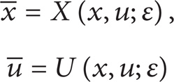
where m > 1 and x = (x₁, x₂, x₃, …, x_n), that is, n independent variables and m dependent variables u = (u¹, u², u³, …, u^m), implies seeking transformations of the form

\begin{matrix} \bar{x} = X (x, u; ε), \\ \bar{u} = U (x, u; ε) \end{matrix}

(7)

generated by the vector field

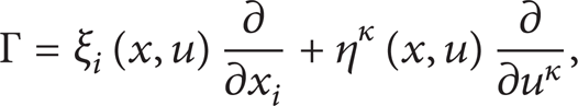
\begin{matrix} Γ = ξ_{i} (x, u) \frac{\partial}{\partial x_{i}} + η^{κ} (x, u) \frac{\partial}{\partial u^{κ}}, \end{matrix}

(8)

which leave the system of the given equations invariant. The symmetry generator (8) is extended to all the derivatives appearing in the system of equations. The infinitesimal criterion for invariance of system of PDEs [12, 13] implies the action

\begin{matrix} Γ^{r} G^{κ} (x, u, u_{(1)}, u_{(2)}, u_{(3)}, \dots, u_{(r)}) = 0 \end{matrix}

(9)

when

\begin{matrix} G^{κ} (x, u, u_{(1)}, u_{(2)}, u_{(3)}, \dots, u_{(r)}) = 0, \\ r = 1,2, 3, \dots, m . \end{matrix}

(10)

Equations (9) yield the determining equations which can be solved algorithmically. The calculations may be facilitated by computer software program such as REDUCE [16], Yalie [17], and DIMSYM [18]. In the initial Lie point symmetry analysis of systems (4) and (5), with S(y, t) being an arbitrary function of y and t, the admitted principal Lie algebra is given by the translation of u. We determine the forms of S(y, t) for which the principal Lie algebra extends. The exercise of searching for the forms of arbitrary functions that extends the principal Lie algebra is called group classification. We adopt the direct methods of group classification as stipulated in [12]. The forms of S and extra admitted symmetries are listed in Table 1.

Table 1:

Extra symmetries admitted by the systems (4) and (5).

Forms of S(y, t)	Parameters	Symmetries

Const.	Arbitrary β = λ	X₂ = ∂ _t, X₃ = ∂ _y X₄ = 2T ∂ _T + (At + u) ∂ _u + (λ + 1)y ∂ _y + 2t ∂ _t

0	Arbitrary β = λ	X₄ = 2At ∂ _u + y ∂ _y + 2t ∂ _t X₅ = 2T ∂ _T + [u – 2A(λ + 1)t] ∂ _u – 2λt ∂ _t

y^ae^−t, a ∈ ℝ	β = λ	X₂ = 2T ∂ _T + (u – At) ∂ _u + λy ∂ _y + (aλ – 2) ∂ _t

(y + a)^bt⁻¹, a, b ∈ ℝ	β = λ	$X_{2} = 2 b T \partial_{T} + [b u - (2 b λ + b - 4) A t] \partial_{u}$ + 2 (y + a) ∂ _y + 2 (1 – bλ) ∂ _t

ay – t, a ∈ ℝ	Arbitrary	X₂ = ∂ _y + a ∂ _t

ty ⁻⁴	Arbitrary λ = β = – 1/2	X₂ = 2At ∂ _u + y ∂ _y + 2t ∂ _t X₃ = – 4T ∂ _T – 2u ∂ _u + 2At ∂ _u + y ∂ _y

x^a, a ∈ ℝ	Arbitrary a = – 2	X₂ = ∂ _t X₃ = 2At ∂ _u + y ∂ _y + 2t ∂ _t

4. Similarity Reductions

Among others, the use of symmetries is to reduce the number of variables of a system of PDEs by one, as such one obtains a system of ODEs. The resulting reduced system may be solved exactly to yield the so-called invariant solutions. Suppose the system of PDEs admits a one-parameter group of transformations (8), and assumingthat ξ(x, u) ≢ 0, the invariant solution admitted by the system of PDEs (6) results from the invariance

\begin{matrix} X (u^{ν} - H (x)) when u = H (x), ν = 1,2, 3, \dots, m, \end{matrix}

(11)

or equivalently

\begin{matrix} ξ_{i} (x, H (x)) \frac{\partial H^{ν}}{\partial x_{i}} = η^{ν} (x, H (x)) . \end{matrix}

(12)

Equation (12) is refered to as the invariant surface condition and its corresponding characteristic equations are given by

\begin{matrix} \frac{d x_{1}}{ξ_{1} (x, u)} = \frac{d x_{2}}{ξ_{2} (x, u)} = \dots = \frac{d x_{m}}{ξ_{m} (x, u)} = \frac{d u^{1}}{η^{1} (x, u)} = \frac{d u^{2}}{η^{2} (x, u)} = \dots = \frac{d u^{m}}{η^{m} (x, u)} . \end{matrix}

(13)

If I₁(x, u), I₂(x, u), …, X_{n – 1}(x, u), andv¹(x, u), v²(x, u), …, v^m(x, u) are the bases of invariants then the invariant solution u = H(x) is given implicitly by the invariant form

\begin{matrix} v^{ν} (x, u) = F^{ν} (I_{1} (x, u), I_{2} (x, u), \dots, X_{n - 1} (x, u)), \end{matrix}

(14)

where F^ν is an arbitrary function of I₁, I₂, …, I_{n – 1}. We consider the following illustrative cases.

Case 1. We consider the symmetry generator X₄ when S = 0 as listed in Table 1. The corresponding characteristic equations are

\begin{matrix} \frac{d u}{2 A t} = \frac{d y}{y} = \frac{d t}{2 t} = \frac{d T}{0} . \end{matrix}

(15)

Thus we obtain the functional form of the invariant solutions given by

\begin{matrix} u = A t + H (γ), T = G (γ), \end{matrix}

(16)

where $γ = (y / \sqrt{t})$ (Boltzmann similarity variable) and H and G satisfy the ordinary differential equations

\frac{d}{d γ} [G^{λ} \frac{d H}{d γ}] + \frac{1}{2} γ \frac{d H}{d γ} = 0,

(17)

\begin{matrix} γ \frac{d G}{d γ} + \frac{1}{Pr} \frac{d}{d γ} [G^{β} \frac{d G}{d γ}] + Ec G^{λ} {(\frac{d H}{d γ})}^{2} = 0 . \end{matrix}

(18)

Note that given λ = 0, then (17) can be solved exactly in terms of the error function.

Case 2. We consider the symmetry generator X₂ when S = ay – t as listed in Table 1. The corresponding characteristic equations are

\begin{matrix} \frac{d y}{1} = \frac{d t}{a} = \frac{d T}{0} = \frac{d u}{0} . \end{matrix}

(19)

Thus we obtain the functional form of the invariant solutions given by

\begin{matrix} u = H (γ), T = G (γ), \end{matrix}

(20)

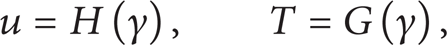
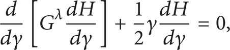
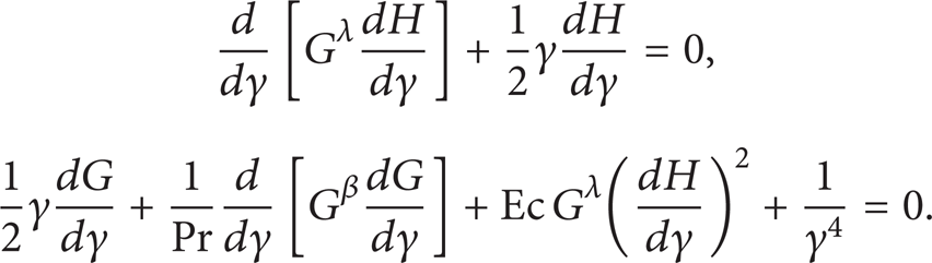
where γ = ay – t (traveling wave type variable) and H and G satisfy the ordinary differential equations

\begin{matrix} a^{2} \frac{d}{d γ} [G^{λ} \frac{d H}{d γ}] + \frac{d H}{d γ} + A = 0, \\ \frac{1}{Pr} \frac{d}{d γ} [G^{β} \frac{d G}{d γ}] + Ec G^{λ} {(\frac{d H}{d γ})}^{2} + a^{2} \frac{d G}{d γ} + a^{2} γ = 0 . \end{matrix}

(21)

Case 3. Given the source term S(y, t) = ty⁻⁴ and symmetry generator X₂ as listed in Table 1, the characteristic equations corresponding to X₂ are given by

\begin{matrix} \frac{d u}{2 A t} = \frac{d y}{y} = \frac{d t}{2 t} = \frac{d T}{0} . \end{matrix}

(22)

Thus we obtain the functional form of the invariant solutions given by

\begin{matrix} u = A t + H (γ), T = G (γ), \end{matrix}

(23)

where $γ = (y / \sqrt{t})$ (Boltzmann similarity variable) and H and G satisfy the ordinary differential equations

\begin{matrix} \frac{d}{d γ} [G^{λ} \frac{d H}{d γ}] + \frac{1}{2} γ \frac{d H}{d γ} = 0, \\ \frac{1}{2} γ \frac{d G}{d γ} + \frac{1}{Pr} \frac{d}{d γ} [G^{β} \frac{d G}{d γ}] + Ec G^{λ} {(\frac{d H}{d γ})}^{2} + \frac{1}{γ^{4}} = 0 . \end{matrix}

(24)

5. Numerical Procedure

In order to demonstrate the solution of the reduced problem in Section 4, the transformed nonlinear ODEs (17) and (18) are tackled numerically by applying the shooting iteration technique together with fourth order Runge-Kutta integration scheme with the prescribed boundary conditions:

\begin{matrix} H (0) = 1, H (\infty) = 0; G (0) = 1, G (\infty) = 0 . \end{matrix}

(25)

It is important to emphasize here that ODEs (17)-(18) together with the boundary conditions (25) correspond to the problem of unsteady thermal boundary layer over a moving heated flat surface with variable properties. Firstly, the model nonlinear boundary value problem in ODEs (17)-(18) together with conditions (25) is reduced to a system of initial value problem. Let

\begin{matrix} H = x_{1}, H^{'} = x_{2}; G = x_{3}, G^{'} = x_{4}, \end{matrix}

(26)

where the prime symbol denotes the derivative with respect to γ. Substituting (26) into (17)-(18) and (25), we obtain

\begin{matrix} x_{1}^{'} = x_{2}, \\ x_{2}^{'} = - λ x_{3}^{- 1} x_{4} x_{2} - \frac{γ}{2} x_{3}^{- 1} x_{2}, \\ x_{4}^{'} = x_{4}, \\ x_{4}^{'} = - β x_{3}^{- 1} x_{4}^{2} - Pr γ x_{3}^{- β} x_{4} - Ec Pr x_{3}^{λ - β} x_{2}^{2}, \end{matrix}

(27)

subject to the following initial conditions:

\begin{matrix} x_{1} (0) = 1, x_{2} (0) = s_{1}, x_{3} (0) = 1, x_{4} (0) = s_{2} . \end{matrix}

(28)

The unspecified initial conditions s₁ and s₂ in (28) are obtained iteratively using the Newton-Raphson algorithm together with fourth order Runge-Kutta integration scheme to a given terminal point. For a fixed set of parameter values, the accuracy of the missing initial conditions was checked by comparing the calculated value with the given value at the terminal point. The computations were done by a written program in MAPLE with a step size of Δγ = 0.001 selected to be satisfactory for a convergence criterion of 10⁻⁷ in nearly all cases. The maximum value of γ_∞ to each group of parameters was determined when the values of the unknown boundary conditions at γ = 0 are not changed to successful loop with error less than 10⁻⁷. From the process of numerical computation, the skin-friction coefficient (-H′(0)) and the local Nusselt number (-G′(0)) are also worked out and their numerical values are presented in tabular form.

6. Results and Discussion

In order to have a clear insight into the physical problem, numerical computations for the representative velocity field, temperature field, coefficient of local skin friction, and the local rates of heat transfer at the moving plate surface have been carried out by assigning some arbitrary chosen specific values to the viscosity variation exponent λ, thermal conductivity variation exponent β, and Eckert number Ec. For our illustrative investigation on unsteady thermal boundary layer past heated moving plate with variable properties, it is assumed that the heat source parameter S = 0 and in order to satisfy the free stream condition, the axial pressure gradient parameter is taken as A = 0. The value of axial pressure gradient parameter Prandtl number is taken as 0.71 (Air) to Pr = 5. For the special case of λ = 0 (i.e., constant viscosity), the exact solution for the unsteady momentum equation (17) together with the boundary conditions (25) is given as (see also [19])

\begin{matrix} H (γ) = erfc (\frac{γ}{2}), \end{matrix}

(29)

where erfc (·) is the complementary error function [20]. In order to validate the accuracy of our numerical procedure in Section 5, we compared the exact solution of the velocity profiles in (29) with our numerical results for the special case of constant fluid viscosity (λ = 0). The numerical results displayed in Table 2 are found to be in excellent agreement with the exact solution in (4).

Table 2:

Comparison between the exact and numerical solution of velocity profile for λ = 0.

γ	H(γ): exact solution	H(γ): numerical solution

0	1	1
0.6	0.6713732405	0.6713732405
1.0	0.4795991222	0.4795991222
1.5	0.2888443663	0.2888443663
2.0	0.1572992071	0.1572992071
3.0	0.0338948535	0.0338948535
4.0	0.0046777350	0.0046777350
6.0	0.0000220905	0.0000220905

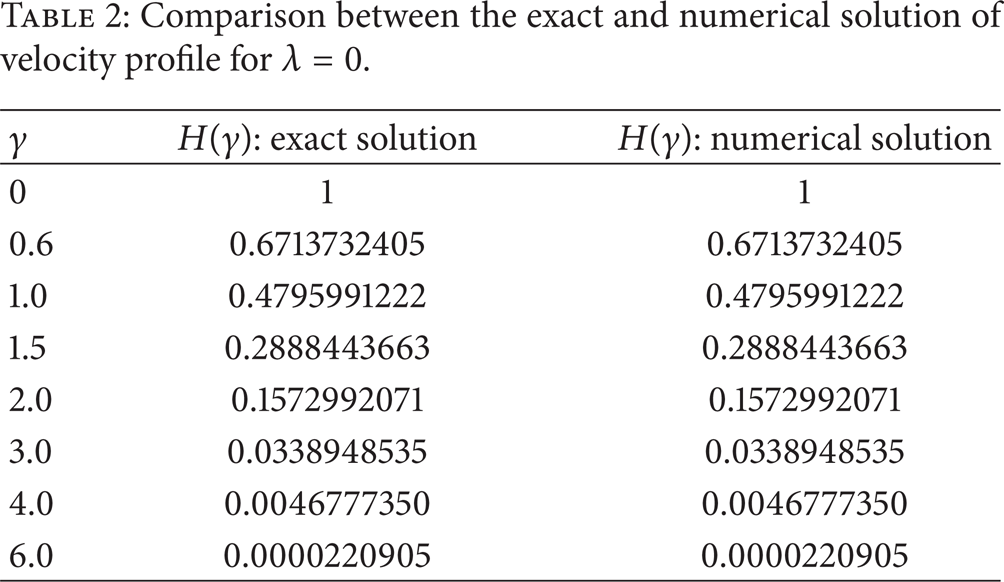
Table 3 uniquely reveals that both the local skin friction and plate surface heat transfer rate are significantly affected by the variation in the thermophysical parameters. As λ increases, the fluid viscosity increases leading to a decrease in the local skin friction and an increase in the heat transfer rate at the moving plate surface. Moreover, a combined increase in the local skin friction and the heat flux at the moving plate surface is observed with increasing fluid thermal conductivity as illustrated (β ≤ 0). It is noteworthy that the local skin friction increases, while the Nusselt number decreases at the moving plate surface with increasing viscous heating represented by Ec > 0. This happens because as the Eckert number increases, the velocity gradient at the plate surface increases leading to an increase in fluid friction at the plate surface. As Prandtl number Pr increases, the skin friction decreases, while the heat transfer at the moving plate surface increases.

Table 3:

Computations for the local skin friction and Nusselt number S = 0 and A = 0.

γ	β	Ec	Pr	-H′(0)	-G′(0)

0	−0.5	0.1	0.71	0.566841	0.870363
1	−0.5	0.1	0.71	0.424639	0.875850
2	−0.5	0.1	0.71	0.353646	0.878839
1	−0.3	0.1	0.71	0.434220	0.750978
1	−0.1	0.1	0.71	0.437599	0.682245
1	−0.5	1.0	0.71	0.434107	0.742653
1	−0.5	1.5	0.71	0.439548	0.439548
1	−0.5	0.1	1	0.411925	0.998206
1	−0.5	0.1	3	0.359723	1.624399
1	−0.5	0.1	5	0.331569	2.075314

6.1. Velocity Profiles

Figures 1 –3 display the boundary layer velocity profiles for different values of variable viscosity exponent (λ), Eckert number (Ec), and Prandtl number (Pr). Generally, the fluid velocity is maximum at the moving plate surface and decreases gradually away from the plate surface to zero value satisfying the prescribed free stream condition. It can be observed from Figure 1 that the velocity of the fluid decreases with the increase in the variable viscosity exponent (λ). This is expected, since as λ increases, the viscosity increases and the fluid becomes heavier leading to a decrease in the velocity profiles and the momentum boundary layer thickness. Similar trend is observed with increasing values of Prandtl number (Pr) as shown in Figure 2. As Pr increases, the momentum boundary layer thickness decreases due to a combined increase in fluid viscosity and decrease in the thermal diffusivity. It can be seen from Figure 3 that the velocity of the fluid increases with an increase in the Eckert number (Ec). This can be attributed to an increase in the fluid velocity gradient due to viscosity heating.

Figure 1:

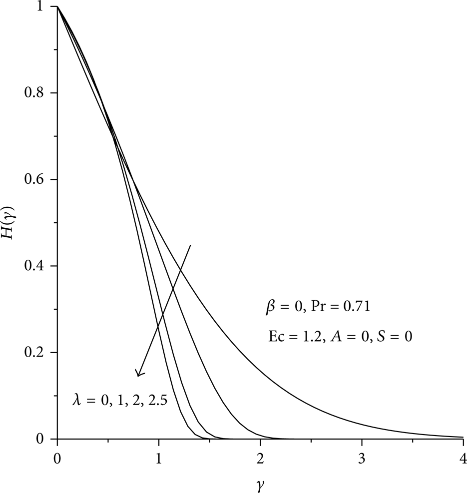
Velocity profiles with increasing viscosity.

Figure 2:

Velocity profiles with increasing Prandtl number.

Figure 3:

Velocity profiles with increasing Eckert number.

6.2. Temperature Profiles

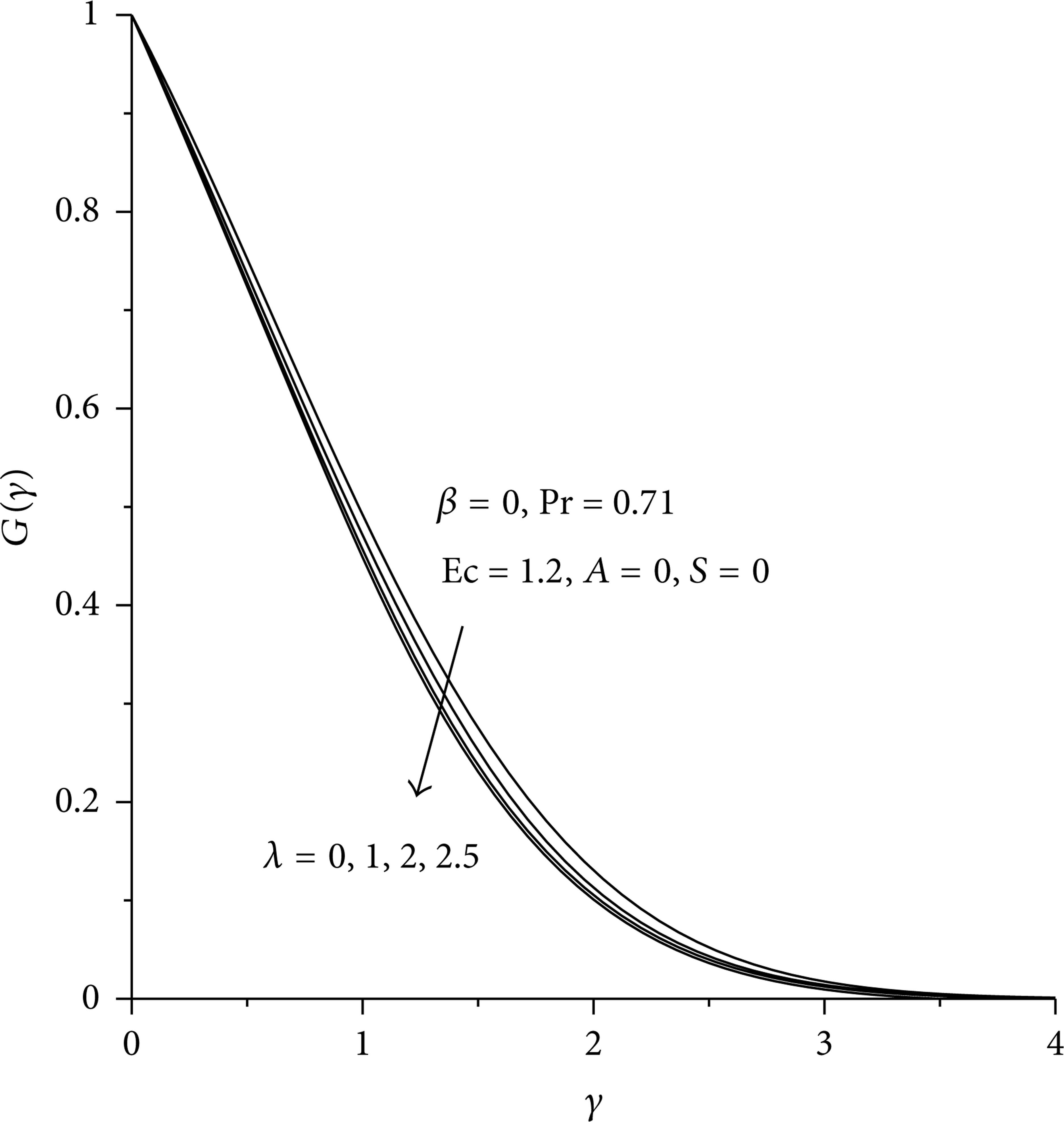
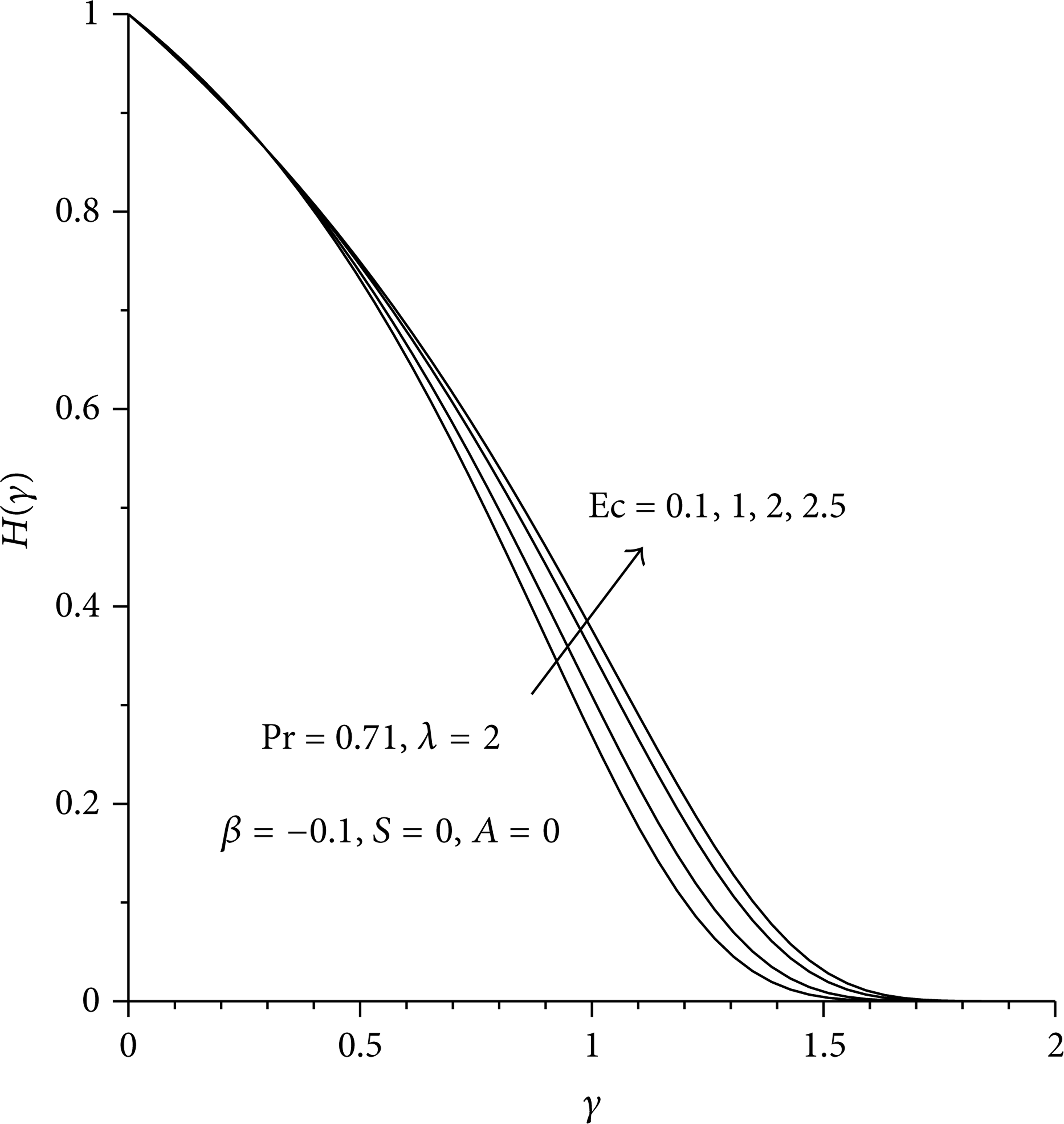
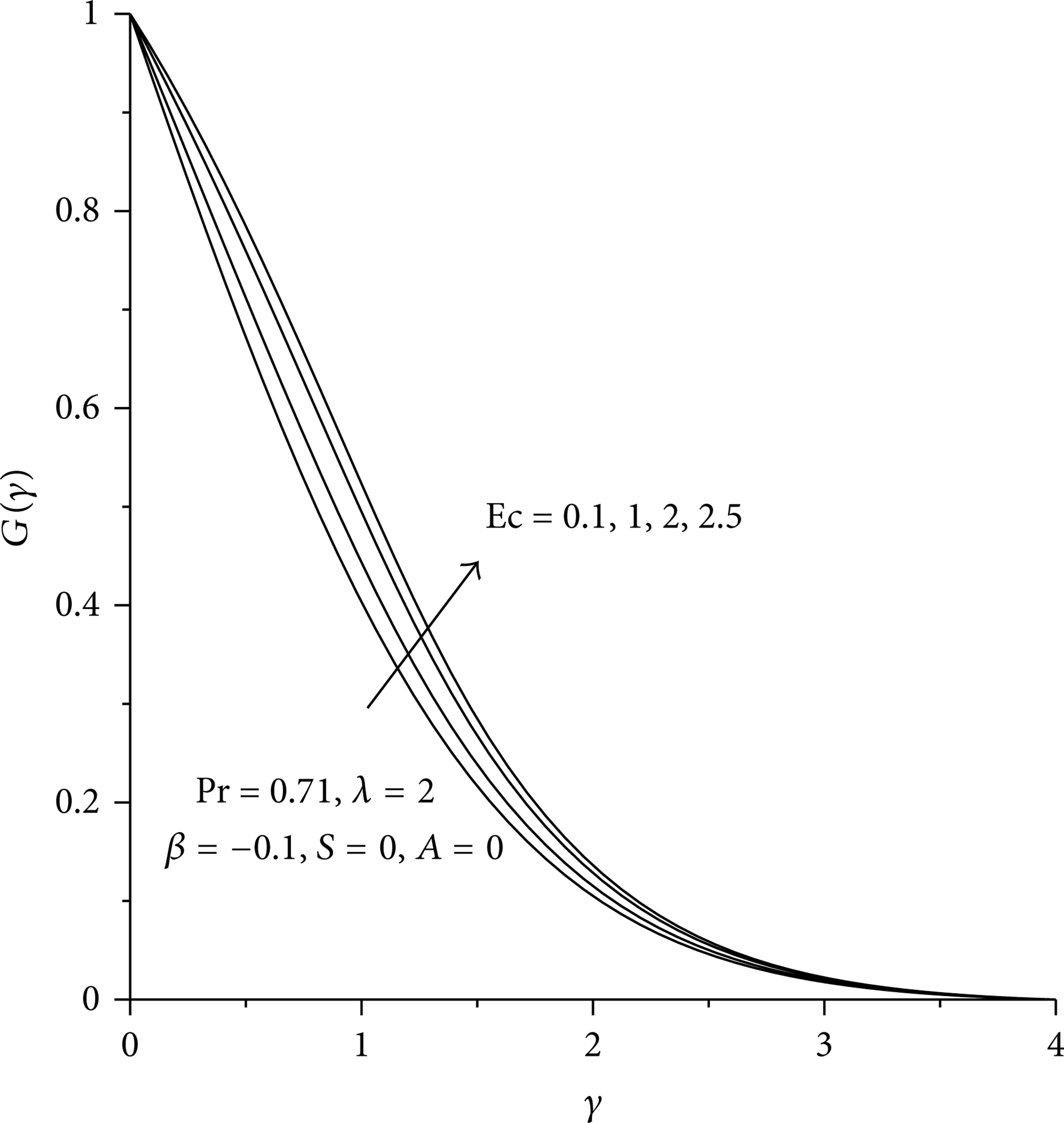
The fluid temperature profile for different thermophysical values is shown in Figures 4, 5, 6, and 7. It is clear that the temperature of the fluid is highest at the heat plate surface and decreases to the prescribed free stream value far away from the plate satisfying the boundary condition. Figures 4 –6 demonstrate the effects of increasing parameters λ, β, and Pr. The thermal boundary layer thickness decreases with a combined increase in fluid viscosity (λ > 0), thermal conductivity illustrated by β ≤ 0, and Prandtl number (Pr > 0). As Ec increases, it can be observed from Figure 7 that the fluid temperature increases; consequently the thermal boundary layer thickness increases. This happens because increasing viscous dissipation effects contributed additional heat to the fluid flow within the boundary layer region.

Figure 4:

Temperature profiles with increasing viscosity.

Figure 5:

Temperature profiles with decreasing thermal conductivity.

Figure 6:

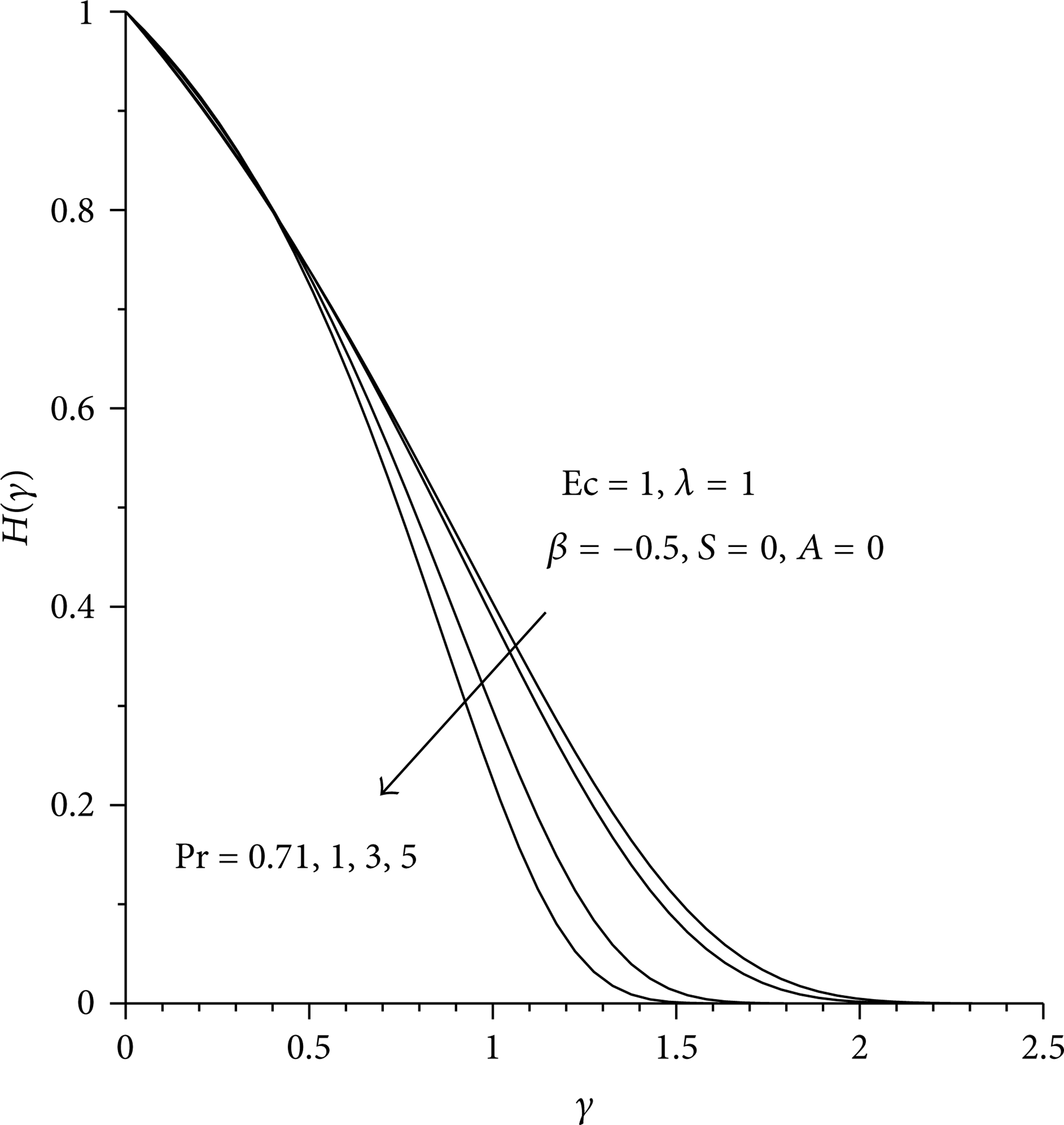
Temperature profiles with increasing Prandtl number.

Figure 7:

Temperature profiles with increasing Eckert number.

7. Concluding Remarks

In this study, we have examined a system of coupled partial differential equations describing unsteady nonlinear fluid flow and heat transfer with variable flow properties using symmetry analysis and Lie algebras. Several transformed nonlinear ordinary differential equations describing unsteady flow and heat transfer problems are obtained. A special case of unsteady thermal boundary layer over a moving flat surface with power law viscosity and thermal conductivity is numerically tackled using shooting quadrature. Numerical results illustrating interesting predicted phenomena were presented graphically and in tabular form. The main conclusions emerging from this study are as follows.

The momentum boundary layer thickness increases with Ec and decreases with λ and Pr.

The thermal boundary layer thickness increases with Ec and decreases with λ, β, and Pr.

The skin friction increases with Ec and β and decreases with Pr and λ.

The Nusselt number increases with β, λ, and Pr and decreases with Ec.

Conflict of Interests

The authors have used the computer software MAPLE for the production of numerical data and plotting of figures. Both the University of the Witwatersrand and the Cape Peninsula University of Technology have acquired user licenses for this software. No funding or even payments were received or made for the production of this paper; as such there is no conflict of interests.

Footnotes

Acknowledgment

The authors wish to thank the National Research Foundation South Africa program for the generous financial support. However, the views and statements made in this paper are entirely the responsibility of the authors.

References

Khound

P. K.

and Hazaika

G. C.

, “The effect of variable viscosity and thermal conductivity on liquid film on an unsteady stretching surface,” in Proceedings of the 46th Annual Technical Session, pp. 47–56, Assam Science Society, 2000.

Andersson

H. I.

Aarseth

J. B.

, and Dandapat

B. S.

, “Heat transfer in a liquid film on an unsteady stretching surface,” International Journal of Heat and Mass Transfer, vol. 43, no. 1, pp. 69–74, 2000.

Tsou

F. K.

Sparrow

E. M.

, and Goldstein

R. J.

, “Flow and heat transfer in the boundary layer on a continuous moving surface,” International Journal of Heat and Mass Transfer, vol. 10, no. 2, pp. 219–235, 1967.

Eswara

A. T.

and Bommaiah

B. C.

, “The effect of variable viscosity on laminar flow due to a point sink,” Indian Journal of Pure and Applied Mathematics, vol. 35, no. 6, pp. 811–815, 2004.

Lai

F. C.

and Kulacki

F. A.

, “The effect of variable viscosity on convective heat transfer along a vertical surface in a saturated porous medium,” International Journal of Heat and Mass Transfer, vol. 33, no. 5, pp. 1028–1031, 1990.

Makinde

O. D.

and Chinyoka

, “MHD transient flows and heat transfer of dusty fluid in a channel with variable physical properties and Navier slip condition,” Computers and Mathematics with Applications, vol. 60, no. 3, pp. 660–669, 2010.

Makinde

O. D.

and Onyejekwe

O. O.

, “A numerical study of MHD generalized Couette flow and heat transfer with variable viscosity and electrical conductivity,” Journal of Magnetism and Magnetic Materials, vol. 323, no. 22, pp. 2757–2763, 2011.

Moitsheki

R. J.

, “Lie group analysis of a flow with contaminant-modified viscosity,” Journal of Applied Mathematics, vol. 2007, Article ID 38278, 10 pages, 2007.

Makinde

O. D.

Moitsheki

R. J.

, and Tau

B. A.

, “Similarity reductions of equations for river pollution,” Applied Mathematics and Computation, vol. 188, no. 2, pp. 1267–1273, 2007.

10.

Moitsheki

R. J.

Abelman

, and Hayat

, “Symmetry reductions of a flow with power law fluid and contaminant-modified viscosity,” Mathematical and Computational Applications, vol. 15, no. 4, pp. 685–696, 2010.

11.

Ivanova

N. M.

and Sophocleous

, “Conservation laws and potential symmetries of systems of diffusion equations,” Journal of Physics A, vol. 14, Article ID 235201, 14 pages, 2008.

12.

Bluman

G. W.

Cheviakov

A. F.

, and Anco

S. C.

, Applications of Symmetry Methods to Partial Differential Equations, Springer, New York, NY, USA, 2010.

13.

Bluman

G. W.

and Anco

, Symmetry and Integration Methods for Differential Equations, Springer, New york, NY, USA, 2002.

14.

Ibragimov

N. H.

, Elementary Lie Group Analysis and Ordinary Differential Equatioons, Wiley, New York, NY, USA, 1999.

15.

Olver

P. J.

, Applications of Lie Groups to Differential Equations, Springer, New York, NY, USA, 1986.

16.

Hearn

A. C.

, “Reduce use manual version 3.4,” The Rand Publication CP78, Santa Monica, Calif, USA, 1985.

17.

Díaz

J. M.

, Short Guide to Yalie: Yet Another Lie Mathematica Package for Lie Symmetries, Wolfram, 2000.

18.

Sherring

, Dimsym: Symmetry Determination and Linear Differential Equation Package, Mathematics Department, Latrobe University, Melbourne, Australia, 1993.

19.

Polyamin

A. D.

and Zaitsev

V. F.

, Handbook of Exact Solution for Ordinary Differential Equations, CRC Press, New York, NY, USA, 1995.

20.

Abramowitz

and Stegun

I. A.

, Handbook of Mathematical Functions, Dover Publication, INC, New York, NY, USA, 1972.

Computational Modelling and Similarity Reduction of Equations for Transient Fluid Flow and Heat Transfer with Variable Properties

Abstract

1. Introduction

2. Governing Equations

3. Classical Lie Point Symmetry Analysis

4. Similarity Reductions

5. Numerical Procedure

6. Results and Discussion

6.1. Velocity Profiles

6.2. Temperature Profiles

7. Concluding Remarks

Conflict of Interests

Footnotes

Acknowledgment

References