
Abstract
Localization, which determines the geographical locations of sensors, is a crucial issue in wireless sensor networks. In this paper, we propose a novel lightweight equilateral triangle localization algorithm (LETLA) that accurately localizes sensors and minimizes the power consumption. In the LETLA, the approximate coordinates substituted for the real coordinates of the unknown node, and the corresponding optimization problem is formulated to minimize the estimation error. With the sequences that represent the ranking of distances from the anchors to the unknown node, a simple and robust technique is developed to quickly and efficiently estimate a region containing the approximate coordinates, and a condition under which the approximate error can be minimized is given. This condition employs a new geometric construct of anchor layout called equilateral triangle diagrams. Extensive simulations show that the LETLA performs better than other state-of-the-art approaches in terms of energy consumption with the same localization precision.
1. Introduction
WSNs (Wireless Sensor Networks) have recently received great attention because they hold the potential to change many aspects of our economy and life [1–8]. Typical networks consist of a large number of densely deployed sensor nodes which could gather local data and communicate with other nodes. The data from these sensor nodes are relevant only if we know their locations. In addition, the accurate location estimation could aid in sensor network services such as routing, information processing, tasking, and querying. Therefore the knowledge of positions becomes imperative [9–17]. Moreover, the minimum resources must be used: typical sensor nodes are battery powered and have a limited processing ability [18, 19]. These constraints impose the new challenges in localization algorithm development and imply that power efficient, computation complexity and location precision should be employed simultaneously. Many methods have been proposed, such as APS (DV-Hop, DV-coordinates) [20], APIT [21–26], triangulation [27–29], Centroid [30–33], Sequence Based [34–38], Voronoi diagrams [39–43], and mathematical programming [44–46].
With regard to the precision of location, most of the localization algorithms can be classified into two broad categories: accuratelocation algorithm and approximate location algorithm. The accuratelocation algorithm produces the exact coordinates of the unknown node through complex calculations and precise measurement of distance. Typical accuratelocation algorithms include triangulation, linear programming, and semidefinite programming. The approximate location algorithms estimate an approximate position of the unknown node, with rough measurement and simple calculation. APS, APIT, Centroid, Sequence Based, and Voronoi diagrams are all approximate location algorithms.
The accurate location algorithms have two major requirements that render them disadvantages; that is, (a) the complexity is high, because triangulation, linear programming, and semidefinite programming usually involve solving higher order nonlinear equations which consume a large amount of energy, and (b) the ranging accuracy should be high enough, otherwise location algorithm will be halted. Under an adverse ranging condition, exact localization is not available; hence the statistical estimation will be introduced [47–49]. When the limited energy, the reduced processor, and the unstable accuracy of ranging results have been given [5, 17, 19], the precise coordinates of the unknown node are usually difficult to be obtained. Furthermore, in the scene of mobile sensor nodes, the precise coordinates need so much time that the location result is not valid anymore.
The approximate location algorithms consume less energy in computing, since the location procedures of APS, APIT, Centroid, Sequence Based, and Voronoi diagrams are made up of simple logical operations and algebraic operations. The aim of approximate location algorithms is to find a rough precise position of the unknown node with the least energy consumption and to achieve a compromise between the accuracy and the complexity. The approximate location algorithms are particularly useful for large-scale wireless sensor networks, because they could extend sensor nodes' life with less computation complexity and energy consumption and tolerate ranging error to a certain degree.
In this paper, we present a novel equilateral triangle localization algorithm (LETLA) that is a lightweight approximate localization algorithm and could provide better precision with less power consumption. In the LETLA, the sensing area is covered by many identical disjoint equilateral triangle diagrams, and the anchors are placed in the vertexes of the equilateral triangle diagrams. The LETLA is an approximate localization based on the concept of substituting the approximate coordinates for the real coordinates, which could loose less accuracy and save more energy. The new geometric construct of the layout, called the equilateral triangle diagrams, has a major contribution to minimize the approximate error and simplify the location procedure. In order to avoid the ranging ambiguities arising from the interference of noise, the LETLA adopts the order of ranging results to represent the location relationship of unknown node and anchors. That is an effective technology and has been employed in many works of literature [34, 36–38].
The rest of the paper is organized as follows. The next section gives a brief overview of the related work. In Section 3, we describe the procedures of the LETLA. To prove the rationality of the LETLA, we calculate the utilization coefficient of the equilateral triangle diagrams, illustrate the geometrical characteristics of the equilateral triangle diagrams, explain the reason for dividing the equilateral triangle into seven distinct regions, and introduce a principle to determine the point of tangency. In Section 4, we demonstrate the localization procedures of the LETLA in a practical scenario. In Section 5, we present a performance study of the LETLA and make a comparison with other four localization techniques. We conclude this paper and mention our future work in Section 6.
2. State of the Art
In this section, we first give a brief summary of centroid, sequence-based, and Voronoi diagrams and then show the inspirations from them.
2.1. Survey of Centroid, Sequence-Based, and Voronoi Diagrams Localization Technology
Recently, many researchers have focused on localization in WSNs. Bulusu et al. [30] demonstrated a location technique called “Centroid” in 2000. Firstly, with the help of basic connectivity or distance information, a rough estimate of relative node distance is made. Then layout of anchors is used to create a relative map of anchor position. Finally the coordinates of the centroid are obtained by calculating the coordinates of anchors which surround the unknown node in a radiation range of communication. The coordinates of the centroid are regarded as the approximate coordinates of the unknown node. In 2007, weighted centroid localization (WCL) was provided by Blumenthal et al. [31]. It is derived from a centroid determination which calculates the position of unknown node by averaging the coordinates of anchors. To improve the precision in real implementations, the weights were used to refine the estimated position [32]. Because the radio device can provide the Link Quality Indication (LQI), received signal strength indication (RSSI), the performance of packet transmission, and even the difference of energy received in packets, it achieves better precision than original centroid localization. In 2011, Jun et al. [33] presented the first theoretical framework for WCL in terms of the localization error distribution parameterized by the node density, the node placement, the shadowing variance, the correlation distance, and the inaccuracy of sensor node positioning. With this analysis, the robustness of WCL has been quantified, and some design guidelines, such as node placement and spacing, for the practical deployment of WCL, have been provided.
Yedavalli et al. [34] described the sequence-based location approach, called Ecolocation, which was quite effective in dense and uniform topologies in 2005. Ecolocation determines the location of unknown nodes by examining the ordered sequence of received signal strength measurements taken at multiple reference nodes. The key features of the Ecolocation algorithm are as follows: (1) it constructs a constraint table based on the RSSI values; (2) it searches the table to find the location. However, the Ecolocation algorithm is imperfect and has a rough localization performance. In 2009, Zhong and He [50] presented a range-free approach to capture a relative distance between 1-hop neighboring nodes from their neighborhood orderings. With little overhead, the proposed method can be conveniently applied as a transparent supporting layer for many state-of-the-art connectivity-based localization solutions.
To improve the localization accuracy, a new algorithm based on the weighted rank order correlation coefficient and the dynamic centroid was proposed by Yu et al. [35] in 2011. The simulations indicate that the localization accuracy and the robustness of the new algorithm are distinctly raised compared with the Ecolocation.
In 2008, Yedavalli et al. [36] introduced a novel sequence-based localization technique (SBL). In the SBL, the localization space can be divided into many distinct regions that can be uniquely identified by the sequences. The sequences represent the ranking of distances from the anchors to that region. The SBL and the Ecolocation are both proposed by Kiran. The Ecolocation picks the location that maximizes the number of satisfied anchor's topology constraints. In contrast, the SBL applies two statistic metrics that capture the difference in the rank orders. For the problem of location error, a new localization technique, based on the SBL, was proposed by Liu et al. [37] in 2009. Because it uses the triangular area which is enclosed by the centroids of the three “nearest” location regions, it improves the accuracy to some extent. In 2011, Hsiao et al. [38] analyzed the deployment strategy of sensor nodes for the SBL algorithm in order to effectively reduce location error such as (1) the standard deviation of the polygon area cut by the perpendicular bisectors should be kept as small as possible; (2) certain amount of space should be maintained between the sensor nodes, and (3) optimization with the angle between the perpendicular bisectors should be utilized.
Voronoi diagrams provide a powerful technique for analysing computational geometric problems. The Voronoi diagrams divide the plane into multiple polygons (known as cells). Specifically, the cells are constructed in the way that any point in a cell is closer to the local site (i.e., the site within the cell) than to any other site on the plane. Recently, the concept of Voronoi diagrams has been applied in robot navigation and map establishing [39].
In 2007, Boukerche et al. [40] proposed a novel approach that adopted Voronoi diagrams. Two types of localization can result from the proposed algorithm: the physical location of the node (e.g., latitude, longitude) or a region limited by the node's Voronoi cell. In 2009, Boukerche et al. improved DV-Hop localization algorithm with Voronoi diagrams to limit the scope of flooding communication and error [41]. In 2010, to achieve “k-coverage” of the sensing area, which means every point in the surveillance area is monitored by at least k sensors, Li and kao [42] presented a novel distributed self-location estimation scheme based on Voronoi diagrams with mobile nodes. Li illustrated that distributed Voronoi diagrams provided a convenient means of analysing the coverage problem in large-scale sensor networks. In the same year, Ampeliotis and Berberidis [43] generalized a notion of the closest point of the approach estimator. While in the closest point of approach estimator, the unknown node may lie close to the closest point of approach node. Hence the unknown node is restricted to lie in a convex set called the sorted order-K Voronoi cell.
2.2. Inspiration of Centroid, Sequence-Based, and Voronoi Diagrams Localization Technology
By the literature in former section, we find some inspirations from centroid, sequence-based, and Voronoi diagrams. They are adopted, developed, and fused in the LETLA.
According to the facts in WSNs, most location applications only require a proximate region instead of the accurate coordinates of the unknown nodes. Especially in the localization of the mobile nodes, the real-time and approximate coordinates of the mobile nodes are more effective than the accurate coordinates with a long computing delay. Moreover, WSNs need to prolong the sensor node's life, as the sensor nodes are powered by batteries and replaced difficultly. Therefore, substituting the approximate coordinates for the real coordinates of the unknown node is an efficient method to balance the location precision and the computation complexity. The purpose of centroid is to substitute the approximate coordinates for the real coordinates, which significantly reduces the location complexity. Enlightened by the centroid, we proposed a method to obtain the approximate coordinates instead of the real coordinates. This method simplifies the arc equations to the tangent equations as described in Section 3.
In WSNs, the unknown nodes can build Voronoi diagrams based on the position information of anchors and the rank of ranging result. Each node also can find the Voronoi diagrams it belongs to. There is a geometric constraint that links the location to the sorting of the distances between the unknown node and the anchors. If we know the correct sorting of the distances, we would restrict the space in which the unknown node may lie. This space is the Voronoi diagrams that corresponds to the correct sorting. Aiming to reduce the computation complexity in building Voronoi diagrams, we propose the equilateral triangle diagrams which have better geometric attribute than Voronoi diagrams in simplifying location process.
The order sequences of ranging result are more robust than the numerical measurement of distance, which has been proved in some papers [34, 36–38]. The measurement noise corrupts the numerical measurement of distance directly and distinctly over the whole location area, but it alters the rank of ranging result slightly in the most of the areas. In the Voronoi diagrams and the equilateral triangle diagrams, each region can be identified by only a sorted sequence of ranging result. Hence, the special limited region covering the unknown node can be determined by the order sequences of ranging result. In some mobile instances, the special limited region can be regarded as a rough location, if a little location delay is demanded. Consequently we apply the sequence-based method in the LETLA to determine the special limited region efficiently.
3. Lightness Equilateral Triangle Localization Method
In the LETLA, the anchors are able to acquire their positions via external device like GPS, but the unknown nodes cannot obtain this information. The unknown nodes can get the positions of the anchors and construct the corresponding location sequence tables. Then, every wireless sensor node is equipped with an omnidirectional antenna which can transfer wireless signal in all directions [21, 50–56].
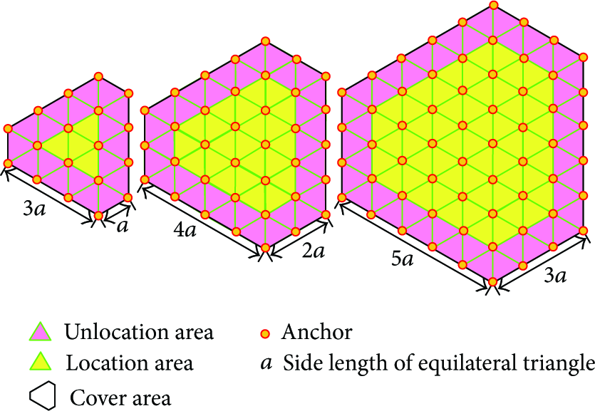
The localization area is divided into many same equilateral triangles, as shown in Figure 1(a). Each equilateral triangle formed by three anchors is picked out to estimate the position of the unknown node. All anchors are deployed in the vertexes of equilateral triangles and fixed after the initial deployment. Each anchor has six adjacent anchors with the same distance, denoted by a. As shown in Figure 1(a), anchor J has six adjacent anchors K, L, M, N, R, and S, which are the nearest six anchors to J with the distance of a. Each node has the same data transmission radius, denoted by l. In the LETLA

Step 1.
The unknown node measures the distances between itself and the anchors in its transmission range and sorts the ranging result in the ascending order. The node P is an unknown node and resides in an equilateral triangle with the side of a. This equilateral triangle can be found by utilizing the three shortest distances between the anchors and node P. If nodes
Step 2.
When
Step 3.
The method of determining the sequence number of the region in

Step 4.
According to the regions including node P in
The method of selecting two arcs to indicate unknown node P with their intersection.

Step 5.
The intersection of the two tangents is substituted for the intersection of two arcs selected in Step 4. In Figure 1(d), the intersection of the two tangents, denoted by Q, is considered to be the approximation of the intersection of two arcs which is also the position of the unknown node P. The principle of finding the point of the tangency is illustrated in Section 3.3.
3.1. Geometrical Characteristics of Equilateral Triangle Diagram
In Step 1, we propose a proposition: the unknown node P resides in
Proposition 1.
As shown in Figure 1(a), if nodes
Proof.
First, in Figure 1(a), the localization space is cut into many equilateral triangles with the same side length a, and therefore each node in the localization space will be inside an equilateral triangle with the side length a. Second, if a node is inside an equilateral triangle, the distances between the node and the three vertexes of the equilateral triangle are all less than the side length
Let us prove this by contradiction. Nodes
3.2. Reason of Dividing Equilateral Triangle
In this section, we will present the reason why
Take
As shown in Figure 1(a),
The definition of the ten divisions in


(a) The angle and the radius of the arc in different regions of
The length of radius in Step 3, denoted by r, is a function of a. Given 

3.3. Principle of Determining Point of Tangency
An arc is determined by the coordinates of center, the length of radius, and the value of angle. In a given arc, a tangent is determined by the position of the point of tangency. Hence, the selection of the tangent is equivalent to choosing an optimization position of the point of tangency. The tangent which touches the arc in the optimal point can minimize the approximation error in Step 4. The gap between the arc and the tangent is a major effect factor of approximation error in Step 5. To facilitate the calculation, a segment of the tangent is used to substitute the whole tangent. As shown in Figure 3,

The definition of
The effects of substituting 
The range of both 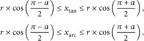
As 
By combining (3) and (5), the following new expression of 
The first indicator is 


By combining (6) and (9), the new expression of 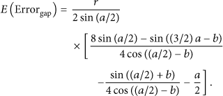
Because syms solve
The numerical result given by MATLAB demonstrates that
The second indicator is 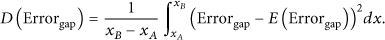
By applying (8) to (11), (12) is obtained:

Combined with (6), (12) can be changed to (13). It is the new expression of 
Because syms solve
The third indicator is 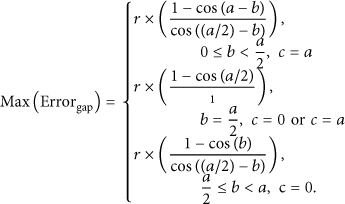
Proposition 2.
As shown in Figure 3 and indicated in (14). If the degree of angle a is constant and the degree of angle b is in the interval
Proposition 3.
As shown in Figure 3 and indicated in (14), if the degree of angle a is constant and the degree of angle b is in the interval
Proof.
Consider
∵
∴
∴
∵
∴
∵
∴
Proof.
Consider
∵
∴
∴
∵
∴
Therefore, if a is given, we can obtain the minimal
Given an arc, the tangent is dominated by the position of the point of tangency. If the point of tangency is the midpoint of the arc, then
3.4. Utilization Coefficient of Equilateral Triangle Diagrams
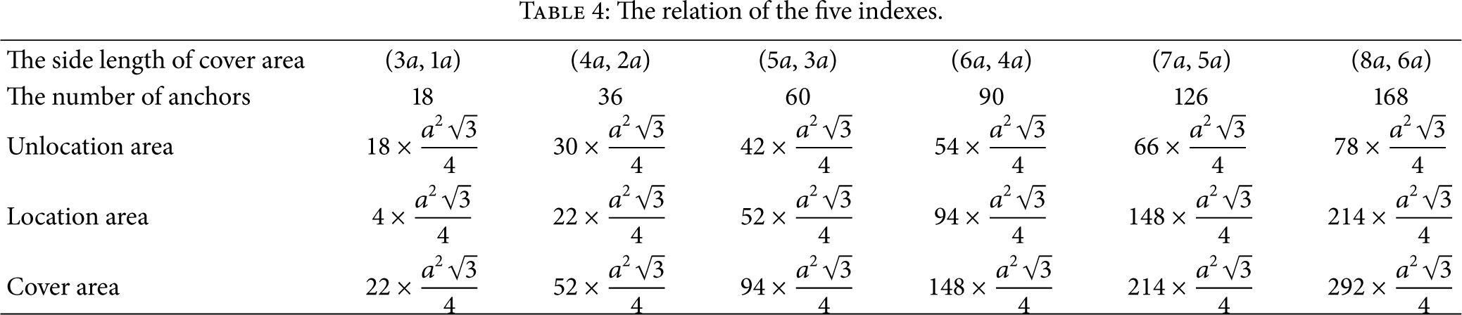
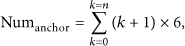
In Step 4, two anchors are selected from the nine anchors which have the special geometrical relations as shown in Figure 1(a). However, it is hard to satisfy the geometrical requirement in the boundaries of the location space. In Figure 4, the location area, unlocation area, and cover area are defined and illustrated in three examples with the sides
The relation of the five indexes.
The topological structure of the equilateral triangle diagrams.


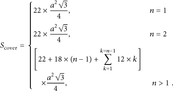
The utilization coefficient of equilateral triangle diagrams is the complement of ratio of 
As (16) and (18) imply,

The utilization coefficient of equilateral triangle diagrams grows along with n's growth.
4. Lightness Equilateral Triangle Localization Algorithm
In this section, the LETLA will be explained by a practical example. This example is shown in Figure 1, and the given conditions are the same as Section 3. When the unknown node P knows the distance between itself and the anchor, the LETLA can be implemented as follows.
Sort the ranging results and select the three nearest anchors Node P finds the regions in As node P is in the fifth region of Derive two tangential equations of the arcs obtained in the previous step and solve the two tangential equations.
The main parameters of a tangential equation include the coordinates of the point of tangency and the slope of tangency. When the tangent is perpendicular to the line which goes through C and the point of tangency K, the slope of tangency can be derived by

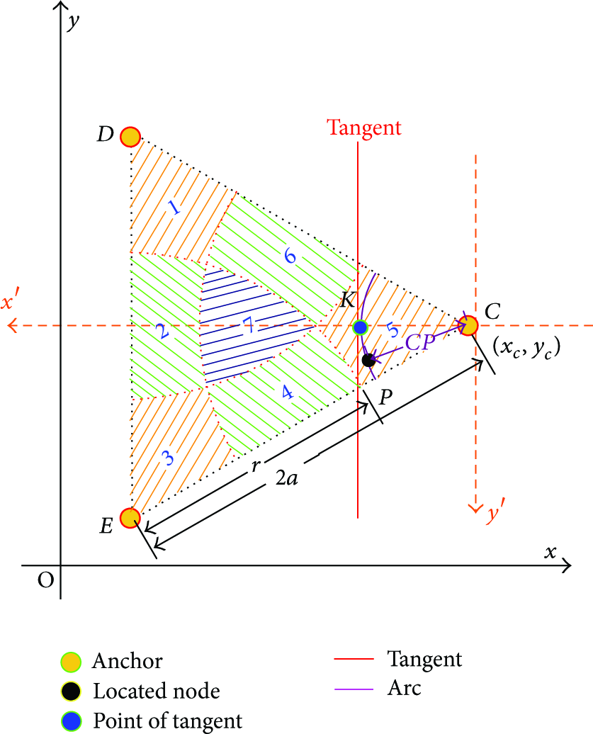
The calculation of the point of the tangent.
The new coordinate system can be built as follows. First, move the original coordinate system to the positive direction of the x-axis with the distance 
The relation of 
Because 
The coordinates of the point of tangency are the function of the coordinates of the center of the arc, the length of radius of the arc, and the angle between the bisector and the x-axis. When the coordinates of the point of tangency are known, the slop of tangency can be drawn from (20). Now the tangential equation can be set up. Solving the intersection of two tangents is equivalent to solving the bivariate system of linear equations.
To sum up, the (a), (b), (c), and (d) in the LETLA are achieved by relational operation and only (e) is implemented by arithmetic operation. The procedure (e) only contains the four arithmetic operations and does not involve solving multivariable nonlinear equations, differentiation, integration, statistical estimation, and mathematical programming. It suggests that the LETLA is a lightness location method.
5. Performance Evaluation
5.1. Localization Error Evaluation
In Section 5.1, a numerical analysis of the performance of localization error will be given. Figure 7 shows the anchor distribution and the coordinate system. It is set up by putting Figure 1(a) in a coordinate system with an origin O on the lower left quarter. In Figure 7, the distance between a pair of adjacent anchors is denoted by a, which is the same in Figure 1(a) and assigned a value of 50. The length of radius to divide

A numerical example of Figure 1(a).
Figure 8 shows the distribution of

The distribution of
In Figure 8,
Figure 9 shows the distribution of

The distribution of
Given
Figure 9 shows that 
By comparing Figures 9 with 8, the range of
5.2. Localization Coverage and Beacon Density
To study the performances of the localization coverage and beacon density, we generate a variety of the test scenarios of the different numbers of anchors. The graphs in Figure 10 illustrate three test scenarios. The whole test area, designed as a circular domain and denoted by 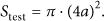

The topological structure of the test scenarios.
The location area
The relationship among the four indexes.

We use the following definitions in the evaluation: localization coverage, 
Because the whole test area is a fixed circular domain, as expressed in (25) and illustrated in Figure 10, the localization coverage increases with growing anchor number, as shown in Figure 11(a). When the number of anchor increases to 91, the location area constitutes 82.699 percent of the test area. Figure 11(b) graphs the beacon density for varying the quantity of anchors under the condition of 
(a) The number of anchors versus localization coverage; (b) the number of anchors versus beacon density.
5.3. Comparisons
We compare the LETLA with the weighted centroid [33], the sequence based [36], the Voronoi diagrams [43], and the multilateration [58]. In order to study the performances of localization precision and energy consumption in different scenarios, NS2 is adopted in Table 6.
The simulation parameters of NS2.

The anchors were deployed uniformly in a square field of 
The most widely used simulation model is the log-normal shadowing model [59], where
In Figure 12(a) the relationship between the localization error and the variance of noise is investigated when the number of anchors is 36. The result shows that the localization error increases with the variance of noise. We can observe that the performance of the multilateration is the best when the variance is less than six. As the variance increases, the LETLA is more robust than the other four algorithms under the same condition. Some of the reasons for this result can be briefly stated. The multilateration will obtain more precise coordinates if the variance becomes smaller. But its performance rapidly degrades when the effect of noise increases. As a result, the circles do not intersect at a common point and the precise coordinates degenerate into the approximate coordinates. The sequence based rises faster than the weighted centroid, the Voronoi diagrams, and the LETLA, since it needs a lot of iterative computations which are sensitive to the initial value. The weighted centroid and the Voronoi diagrams rise gently, but they are less accurate than the LETLA, because they have not fully utilized the information of the anchor placement.

(a) The relationship between the localization error and the variance of noise; (b) the relationship between the localization error and the number of anchors.
In Figure 12(b), the localization error decreases with the increment of anchors, when the variance of noise is ten. As the number of anchors increases, the density of anchors also grows in the fixed cover area. For this reason the received signal power is enhanced with the decrement of the distances between the anchors and the unknown node. As shown in Figure 12(b), the sequence based, the LETLA, and the Voronoi diagrams descend in steps. The reason is that a few increments of the number of anchors are not sufficient to change the density obviously. Only some degrees of promotion can alter the density adequately and improve precision effectually. It is also interesting to note that the Multilateration is the best when the number of anchors less than 32. However, as anchors began to accumulate, the LETLA, the Voronoi diagrams, and the multilateration are of about the same accuracy.
Figure 13 presents the energy consumptions of five algorithms when the variance of noise is ten. Under the same condition, the multilateration consumes more energy than the other four methods. The multilateration with noisy data as described above is based on solving nonlinear equations with complicated closed-form solutions. However, standard algorithms that provide least-square solutions for large numbers of nonlinear equations have a very high computational cost.

The energy consumption in the localization calculation versus the number of anchors.
In Figure 13 the tendency of the weighted centroid, the sequence based, and the Voronoi diagrams rise with the number of anchors and the energy consumptions of these three methods are less than the multilateration but more than the LETLA. By studying the References [33, 36, 43], we can find some reasons. The Voronoi diagrams spend most of the computing energy in constructing Voronoi diagrams and carrying out iterative computations [43]. The sequence based consumes too many energy in the generalization of location sequence tables and the calculation of the Spearman's Rank Order Correlation Coefficient and the Kendall's Tau [36]. The weighted centroid does not contain iterative computation, so it is simpler than sequence based and Voronoi diagrams. However, the Weighted Centroid has more energy consumption for solving the constrained extremum problems [33].
On the other hand, the energy consumption of the LETLA is the least of all. As mentioned in Section 4, the LETLA only solves binary linear equations, except matching and sorting in a limited range, and does not contain any iterative computations, statistical equilibrium, and multivariate nonlinear equations. It is worthwhile to note that, the energy consumption of the LETLA is stable. There are two reasons. First, only two of the nine ranging results and the coordinates of anchors are used to construct and solve the binary linear equations. It means that the scale of the calculation of the LETLA is fixed and limited. Second, the matching and sorting operations can be implemented with the special data structure, like index point, which trades time for space. In contrast with the weighted Centroid, the sequence based, the Voronoi diagrams, and the multilateration, the results suggest that the LETLA is more energy efficient with the same localization accuracy.
6. Conclusion
In this paper, we presented a novel lightness equilateral triangle localization algorithm (LETLA). In the LETLA, the approximate coordinates were substituted for the real coordinates of the unknown node and an optimization problem was set up to minimize the approximate error. To solve this optimization problem, we proposed a new geometric structure called “equilateral triangle diagrams.” In detail, we probed into the scalability of equilateral triangle diagrams and presented the geometrical characteristic of equilateral triangle diagrams. In the process of substituting the tangent for the arc, we derived that the midpoint of the arc was the most appropriate position of the point of the tangent.
Finally, the performance of the LETLA is much better than those of the other localization techniques, and experimental results indicate that the energy consumption of the LETLA is less than other location algorithm, at the same degree of location precision. As part of future work, we would focus on the implementation of the LETLA in the practical hardware of sensor nodes, such as MicaZ, Mica2, and Telos.
Footnotes
Acknowledgments
The authors would like to thank the anonymous reviewers for their helpful comments which have significantly improved the quality of the paper. This work was supported in part by NSFC under Grant no. 60973022.