Sage Journals: Discover world-class research

Abstract

Predicting cooling load for the next 24 hours is essential for the optimal control of air-conditioning systems that use thermal cool storage. This study investigated modeling methods of applying the general regression neural network (GRNN) technology to predict load. The single stage (SS) and double stage (DS) prediction methods were introduced. Two SS and two DS models were set up for forecasting the next 24 hours' cooling load. Measured data collected from two five star hotels located in Sanya, China, were used to train and test these models. The results demonstrate that the SS method, which can eliminate the necessity for measuring and predicting meteorological data, is much simpler and reliable for predicting the cooling load in practical applications.

1. Introduction

Accurate prediction of the building cooling load is a key for optimal control of air-conditioning systems. It is useful to adjust the starting time of cooling to meet start-up loads, minimize the electric on-peak demand, and optimize costs and energy use for cool storage systems and related energy and cost needs in other air-conditioning systems. Lu et al. [1] have shown that an optimal integrity scheme based on cooling load prediction significantly improves the operating cost of a large multichiller system. Kawashima and Dorgan [2] described an ice storage system, which has a controller with load prediction by neural networks, that reduced the total operating costs by 12.5%.

However, accurately predicting the building cooling load is a challenging work. The cooling load is affected by many factors, and it is difficult to consider all of them very well in the load prediction process. Artificial neural network (ANN) is widely accepted as a technology offering a convenient way to tackle complex and ill-defined problems. Hence, it was popularly applied to predict the building cooling load [3 –5], and its capability for predicting load has been examined over conventional technologies, such as regression analysis and time series [6]. Li et al. [7] compared different kinds of ANNs, and found that the general regression neural network (GRNN) algorithm is more effective than the back propagation neural network (BPNN) and the radial basis function neural network (RBFNN) algorithm.

The building cooling load is strongly linked to the outdoor weather. Meteorological parameters are the main load factors. Most reported load models predicted cooling load based on meteorological parameters, such as ambient temperature, relative humidity, solar radiation, wind speed, and sky condition. As far as it concerns predicting the next 24 hours' cooling loads, the weather data for the next 24 hours must be predicted in advance. Therefore, it is a double stage (DS) prediction method to model cooling load. The first stage is to forecast meteorological data, and the second stage is to predict load. Although the DS method has achieved some success, the predictive control system will be too complicated to measure and predict many meteorological parameters.

Single stage (SS) prediction method is a more simple modeling method, which predicts the cooling load for the next 24 hours directly, eliminating the necessity of hourly weather forecasting. It has been investigated by a few researchers. Karatasou et al. [8] employed historical data of the load and ambient temperature to predict load, and Ben-Nakhi and Mahmoud [9] only used the last 24 hours' ambient temperature readings as network inputs. Compared with the DS method, the SS method is obviously easy to build load prediction model for the control system. But whether the SS method for the next 24 hours' loads prediction can be more effective than the DS method, little information can be available.

The main objective of this study is to investigate an agreeable approach for modeling and predicting the next 24 hours' cooling loads. GRNN was applied to set up load prediction models for its quick learning and excellent fitting ability. Two SS models and two DS models were built according to different modeling methods and input variables. Two large hotels located in Sanya, China, were selected to test and validate these models. The predictive performances were compared and the optimal model was discussed.

2. GRNN Algorithm

The GRNN is a kind of radial basis function networks developed by Specht [10]. It is a powerful regression tool with a dynamic network structure. It approximates any arbitrary function between the input and output vectors, drawing the function estimation directly from the training data. The main advantage is the extremely rapid training, which does not require an iterative training procedure.

A typical GRNN mainly has four layers, as presented in Figure 1. When nonlinear regression is performed, each layer is assigned to a specific computational function. The first layer of the network is used to receive information, and there is a unique input neuron for each input variable.

Figure 1:

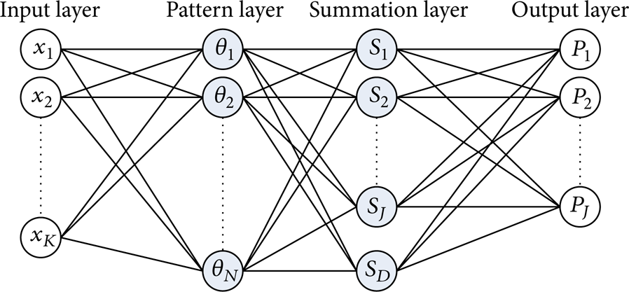
Fundamental structure of a GRNN.

The second layer is used to combine and process the input data in a systematic fashion so that the relationship between the input and the proper response is “memorized.” Therefore, the neurons in the second layer are also called pattern neurons, and the number of pattern neurons (N) is equal to the number of training samples. A typical pattern neuron i obtains the data from the input neurons and computes an output θ_i by using a multivariate Gaussian function given in (1), where U_i is the specific training vector represented by pattern neuron i, and σ is the smoothing factor, consider

\begin{matrix} θ_{i} = \exp [\frac{- {(X - U_{i})}^{'} (X - U_{i})}{2 σ^{2}}], i = 1,2, \dots, N, \end{matrix}

(1)

where σ is a parameter that should be set by the user. When σ is made larger, the estimated density is forced to be smooth and in the limit becomes a multivariate Gaussian with covariance σ². On the other hand, a smaller value of σ allows the estimated density to assume non-Gaussian shapes, but with the risk that the outlying data points may have too great an effect on the estimate.

In the third layer, the neurons, named the summation neurons, receive and augment the outputs of the pattern neurons. Technically, there are two types of summations, simple arithmetic summations and weighted summations, performed in the summation neurons, which can be represented as (2) and (3), respectively as follows:

S_{D} = \sum_{i = 1}^{N} θ_{i},

(2)

\begin{matrix} S_{j} = \sum_{i = 1}^{N} w_{i j} θ_{i}, j = 1,2, \dots, J, \end{matrix}

(3)

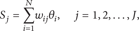
where w_ij is the weight between pattern neuron i and third layer neuron j.

The summations of the neurons in the third layer are subsequently sent to the fourth layer. The regression output of GRNN is calculated as follows:

\begin{matrix} P_{j} = \frac{S_{j}}{S_{s}}, j = 1,2, \dots, J . \end{matrix}

(4)

Data on input and output layers should be normalized before being used in the GRNN, to improve the calculation efficiency, and prevent individual data from overflowing during the calculation. Equations (5) and (6) normalize the input and output variables to the interval [−1,1], respectively, as follows:

{x_{i}}^{'} = 2 \times \frac{x_{i} - x_{i}^{\min}}{x_{i}^{\max} - x_{i}^{\min}} - 1,

(5)

\begin{matrix} {y_{i}}^{'} = 2 \times \frac{y_{i} - y_{i}^{\min}}{y_{i}^{\max} - y_{i}^{\min}} - 1, \end{matrix}

(6)

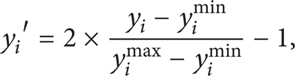
where x_i is an input variable, y_i is an output variable, x_i^max and x_i^min are the maximum and minimum values of x_i, y_i^max and y_i^min are the maximum and minimum values of y_i, and x_i′ and y_i′ are the normalized input and output variables.

After the regression output P is obtained from GRNN model, it should be transformed into the actual prediction value ${\hat{y}}_{i}$ by

\begin{matrix} {\hat{y}}_{i} = \frac{(P_{i} + 1)}{2} \times (y_{i}^{\max} - y_{i}^{\min}) + y_{i}^{\min} . \end{matrix}

(7)

3. Single Stage Load Prediction Models

There is only a one-stage prediction in the single stage (SS) method for the next 24 hours' cooling load prediction. It is primarily based on time series analysis, which takes observed data series to forecast future data. In this section, 2 SS GRNN models (S-1 to 2) based on different inputs were set up, as shown in Table 1.

Table 1:

Input and output variable settings of SS load mode.

Models	Input	Output

S-1	${T_{i, d - 1}}_{i = 1}^{24}$	${Q_{i, d}}_{i = 1}^{24}$
S-2	$({Q_{i, d - 1}}_{i = 1}^{24}, T_{d}^{high}, T_{d}^{low}, {SC}_{d})$	${Q_{i, d}}_{i = 1}^{24}$

The SS load model developed by Ben-Nakhi and Mahmoud [9] was introduced, named as S-1. The input vector is $X = {T_{i, d - 1}}_{i = 1}^{24}$ , that are hourly ambient temperatures from the previous day. The output vector is $P = {Q_{i, d}}_{i = 1}^{24}$ , which are hourly cooling loads for the next day. Model S-1 predicts cooling load only based on historical ambient temperature data.

Furthermore, a new SS load model was proposed, named as S-2. Considering that the cooling load is the result of all load factors on the building, and it changes periodically with a period of 24 hours, the load time series data ${Q_{i, d - 1}}_{i = 1}^{24}$ might contain more information than ${T_{i, d - 1}}_{i = 1}^{24}$ for load prediction. Model S-2 uses the 24 hours' load of the previous day ${Q_{i, d - 1}}_{i = 1}^{24}$ as the main input variables. In addition, tomorrow's high and low temperatures (T_d^high, T_d^low) and sky condition (SC_d), which are issued by the meteorological center, are also introduced to the load model. Therefore, the input vector of model S-2 is $X = ({Q_{i, d - 1}}_{i = 1}^{24}, T_{d}^{high}, T_{d}^{low}, S C_{d})$ , the output vector is the same as that of model S-1.

4. Double Stage Load Prediction Models

Double stage (DS) prediction method was used to set up load GRNN models to compare with the SS load models. The DS load models have two stage predictions. At the first stage, meteorological data for the next 24 hours are forecast. At the second stage, cooling loads for the next 24 hours are predicted based on the outputs of the first-stage prediction.

4.1. First Stage—Weather Forecast

GRNN algorithm is also suitable to predict hourly weather data for the nonlinearity in climate physics [11]. In this study, the main meteorological parameters, including ambient temperature (T), relative humidity (H), and solar radiation intensity (I), were chosen for load prediction. Three weather forecasting models (D-T, D-H, and D-I) were set up based on GRNN, as shown in Table 2.

Table 2:

Weather models for predicting ambient temperature, relative humidity, and solar radiation intensity.

Models	Input	Output

D-T	${T_{i, d - 1}}_{i = 1}^{24}, T_{d}^{high}, T_{d}^{low}, {SC}_{d}$	${T_{i, d}}_{i = 1}^{24}$
D-H	${H_{i, d - 1}}_{i = 1}^{24}, T_{d}^{high}, T_{d}^{low}, {SC}_{d}$	${H_{i, d}}_{i = 1}^{24}$
D-I	${I_{i, d - 1}}_{i = 1}^{24}, T_{d}^{high}, T_{d}^{low}, {SC}_{d}$	${I_{i, d}}_{i = 1}^{24}$

Because the weather prediction is a temporal and time-series-based process, each model uses historical 24 hours' data as the main input variables, and the next 24 hours' values as the output. Tomorrow's weather forecasts (T_d^high, T_d^low, SC_d) were also employed to improve the predictive accuracy.

4.2. Second Stage—Load Prediction

Two DS load models (D-1 and D-2) were established according to the reported studies. The details are given in Table 3. Both DS load models choose Q_τ, cooling load at the target time τ, as the output, and employ meteorological parameters as the main input variables.

Table 3:

Input and output variable settings of DS load models.

Models	Input	Output

D-1	$τ, {T_{i}}_{i = τ - 2}^{τ}, H_{τ}, {I_{i}}_{i = τ - 1}^{τ}$	Q _τ
D-2	$τ, {T_{i}}_{i = τ - 2}^{τ}, H_{τ}, {I_{i}}_{i = τ - 1}^{τ}, Q_{τ, d - 1}$	Q _τ

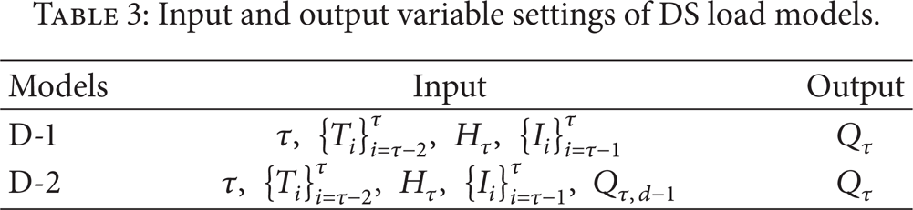
Model D-1 only uses meteorological parameters to predict cooling load. The input vector is $X = (τ, {T_{i}}_{i = τ - 2}^{τ}, H_{τ}, {I_{i}}_{i = τ - 1}^{τ})$ . ${T_{i}}_{i = τ - 2}^{τ}$ represents the ambient temperatures at the time of τ, τ – 1, τ – 2; H_τ is the relative humidity at the time of τ; and ${I_{i}}_{i = τ - 1}^{τ}$ are the solar radiation intensity at the time of τ, τ – 1. The selection of input variables has taken account of the delay of meteorological parameters' influence on the dynamic cooling load, and its rationality has been validated by Shi et al. [12] and Li et al. [13].

Model D-2 introduces historical load in the input. Compared with D-1, model D-2 adds an input variable Q_{τ, d – 1}, which is the cooling load at the target time τ of the previous day. Kawashima et al. [6] have used the same input and output to build a BP load model, and got good predictive accuracy.

There are meteorological input variables that have the time stamps τ, τ – 1, τ – 2 in the DS load models. But the next 24 hours' weather data are unknown in an operating situation; DS load models have to use the estimated weather data to predict the next 24 hours' cooling loads.

5. Load Prediction Models' Application

5.1. Buildings and Measured Data

Two large hotels (hotels A and B) located in Sanya, China, were selected to validate the performance of the SS and DS load prediction models. Table 4 gives basic information of the two hotels.

Table 4:

Basic information on the buildings.

Building	Gross floor area (m²)	Air-conditioning area (m²)	Design cooling load (kW)

Hotel A	50000	40000	4043
Hotel B	60030	48830	5485

Both hotels are users of a district ice-storage cooling plant. As Sanya is in the tropical oceanic monsoon climate area, the cooling systems of hotels run continuously throughout the year.

Measurements at both hotels were taken by a building automation system at short time intervals. The cooling load of each hotel was measured by a cooling meter (accuracy: class two). The ambient temperature and relative humidity were measured by an outdoor temperature/humidity sensor (accuracy: ±0.5°C and ±2% RH), and the solar radiation intensity was measured by a solar radiometer (accuracy: 10 W/m²). Tomorrow's weather forecasts (T_d^high, T_d^low, SC_d) were obtained from the website of Sanya Meteorological Bureau. The sky condition (SC_d) is typically sunny, cloudy, showers and rainy, which are expressed as levels 1, 2, 3, and 4, respectively.

Measured data were collected for about a year. The dataset of hotel A is from June 2011 to April 2012, and that of hotel B is from July 2011 to August 2012. Figure 2 shows the measured cooling load for the two hotels.

Figure 2:

Measured cooling load of hotels.

Each dataset was divided into two parts for training and testing GRNN prediction models. For hotel A, the data in April 2012 (30 days) were kept as the testing samples, and other data from June 2011 to March 2012 (295 days) were used as the training samples. For hotel B, the data in July and August 2012 (62 days) were kept as the testing samples, and other data from July 2011 to June 2012 (365 days) were used as the training samples.

5.2. Performance Indices

The performance evaluation indices to the GRNN models throughout this study are the expected error percentage (EEP) and the coefficient of correlation (r), which are defined by (8) and (9), respectively, as follows:

EEP = \frac{\sqrt{(\sum_{i = 1}^{N} {(p_{i} - y_{i})}^{2}) / N}}{| y_{\max} |} \times 100 %,

(8)

\begin{matrix} r = \frac{\sum_{i = 1}^{N} (y_{i} - \overset{—}{y}) (p_{i} - \overset{—}{p})}{\sqrt{\sum_{i = 1}^{N} {(y_{i} - \overset{—}{y})}^{2} \sum_{i = 1}^{N} {(p_{i} - \overset{—}{p})}^{2}}}, \end{matrix}

(9)

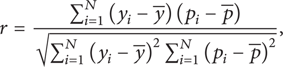
where N is the total number of samples, y_i and p_i are the target and the predicted values, respectively, $\overset{—}{y}$ and $\overset{—}{p}$ are the means of the target and the predicted values, respectively, and y_max is the maximum measured values.

5.3. Parameter Setting

There is only one parameter, the smooth factor (σ), which can be adjusted in GRNN models. Stepwise searching and leave-one-out cross-validation method [10] can be used to select the optimal value of σ for each GRNN model.

In this study, the initial value of σ is set to 0.1, and the step-length is 0.01. The GRNN models with various parameter settings were trained using the training samples, and the prediction error values of EEP were recorded. The results are shown in Figure 3.

Figure 3:

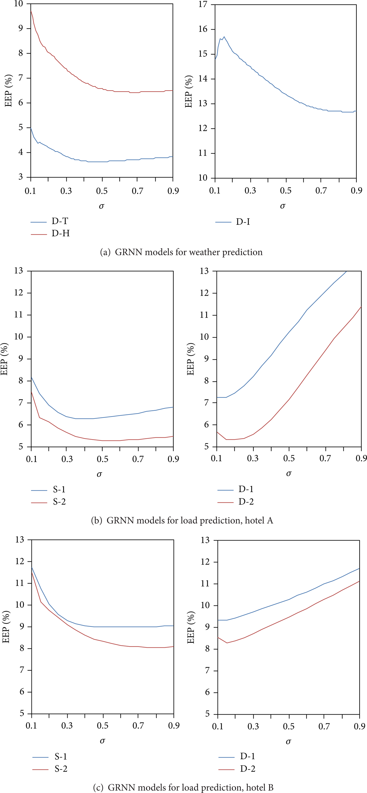
The results of GRNN models with various σ.

It clearly shows that the parameter σ has great effect on the predictive accuracy of a GRNN model. The optimal σ was determined according to the lowest point on the prediction error curve of each model, and results are given in Table 5.

Table 5:

Parameter settings of GRNN models.

Model (weather)	σ	Model (hotel A)	σ	Model (hotel B)	σ

D-T	0.47	S-1	0.40	S-1	0.60
D-H	0.68	S-2	0.55	S-2	0.80
D-I	0.85	D-1	0.15	D-1	0.10
		D-2	0.20	D-2	0.15

5.4. Results and Discussion

GRNN models were established on the training samples after determining parameter σ. They were used to predict the cooling load for hotel A and B. The results are shown in Tables 6 and 7. Moreover, Figures 4 and 5 give examples of the predicted cooling loads for the two hotels, respectively.

Table 6:

Results of cooling load predictions for hotel A.

Model	June 2011–March 2012 (training sample)		April 2012 (testing sample)
Model	EEP (%)	r	EEP (%)	r

S-1	6.3	0.937	9.6	0.834
S-2	5.3	0.955	7.7	0.898
D-1	7.2	0.915	9.1	0.853
D-2	5.3	0.955	7.7	0.896

Table 7:

Results of cooling load predictions for hotel B.

Model	July 2011–June 2012 (training sample)		July-August 2012 (testing sample)
Model	EEP (%)	r	EEP (%)	r

S-1	9.0	0.780	12.6	0.652
S-2	8.1	0.828	10.9	0.760
D-1	9.3	0.770	12.2	0.679
D-2	8.3	0.824	10.9	0.755

Figure 4:

Hourly cooling load prediction for hotel A (April 2012).

Figure 5:

Hourly cooling load prediction for hotel B (July 2012).

It clearly shows that models S-1 and D-1, which only use weather data to predict cooling load, have unacceptable performance. Because the building cooling load is very complicated, the information of weather parameters cannot be satisfied for load models to predict cooling load accurately.

Models S-2 and D-2 both improve their predictive performance for introducing historical load in the input. In the testing course, Model S-2 reduces the expectation of error percentage by 20% (13.5%) for hotel A (B) compared with model S-1, and Model D-2 reduces the EEP by 15% (10.5%) for hotel A (B) compared with model D-1. Such significant improvement is also found in the training course. Therefore, historical load data play an important role in cooling load prediction.

Model S-2, which uses the SS prediction method to set up, have almost the same high predictive accuracy as model D-2, which is built based on the DS prediction method. The SS prediction method was demonstrated to be effective for cooling load prediction. Model S-2 predicts cooling load only based on historical load and tomorrow's weather forecasts issued by meteorological center. The necessity of measuring and predicting hourly meteorological data is eliminated. It cannot only reduce the construction investment in the building automation system but also decreases the instability of prediction caused by weather sensor faults. Therefore, the SS load model S-2 is much more simple and reliable for predicting the cooling load in practical applications.

In the testing course, Model D-2 used the predicted weather data to predict the cooling load. In addition, Model D-2 with measured weather data was also studied. It is found that there is little difference in predictive accuracy. Hence, the GRNN weather models have enough predictive accuracy for cooling load prediction.

Furthermore, the influence of the training sample amount on load prediction was investigated. Figure 6 shows the prediction error curve of model S-2 and D-2 with various amounts of training sample. It can be seen that both models have good learning ability, working well even in a small data amount. As the data amount of similar load conditions increases, the predictive accuracy of both models will be further improved.

Figure 6:

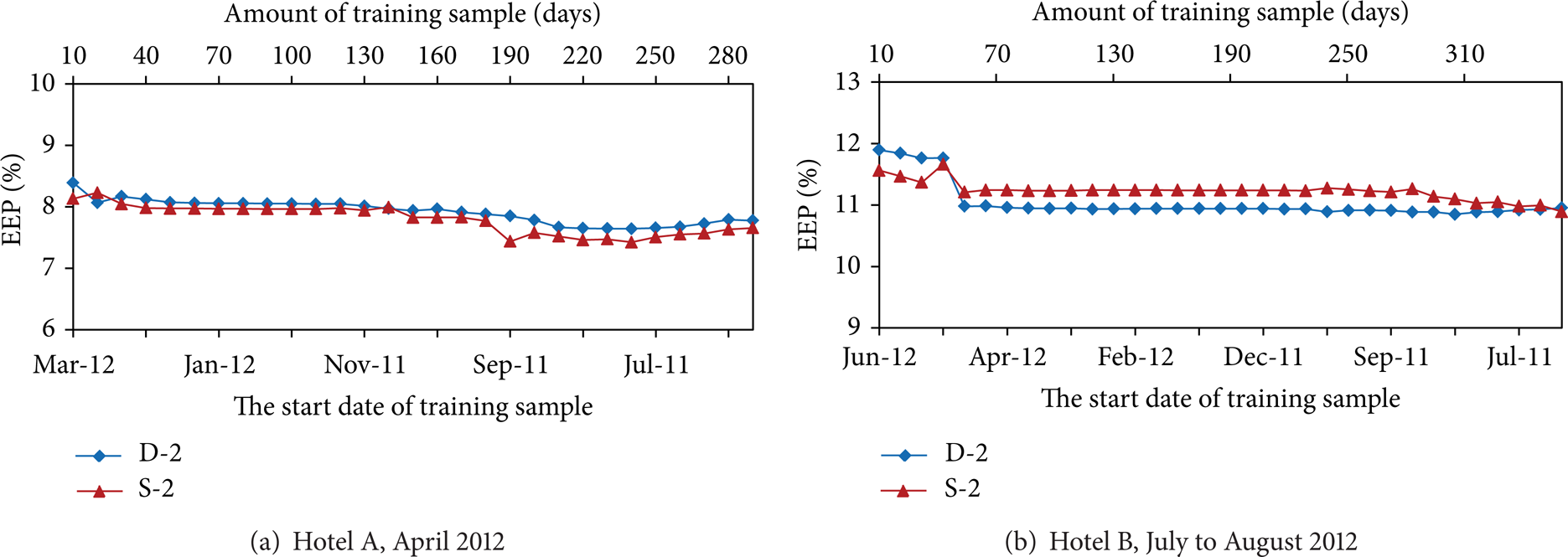
The prediction error of load models with various amounts of training sample.

In Figures 4 and 5, the predicted loads of models S-2 and D-2 have better agreement with the measured loads than model S-1 and D-1. But, it can be seen that the actual cooling load of two hotels often changes dramatically, and load models established in this study are still unsatisfactory for predicting this great change of load.

6. Conclusions

In this study, GRNN was applied to predict the next 24 hours' cooling loads. Two DS and two SS prediction models based on GRNN were set up with different inputs. Two different measured data sets were used to validate these models. The performance indices were represented by the expected error percentage and coefficient of correlation.

The load models, which only employ hourly weather forecast data as network inputs, were found to be far from satisfactory for predicting cooling load, due to the complex of load factors in real buildings. Historical load plays an important role in building cooling load prediction, and its introduction can improve the predictive accuracy significantly. The SS load prediction method is effective for load prediction. The SS model S-2 gets the same good performance as the best DS model D-2. Model S-2 uses the previous 24 hours' loads and tomorrow's weather forecasts issued by meteorological center as the network input, and the next 24 hours' loads as the output. It is simple to establish and apply in practical applications.

In real buildings, the cooling load has dramatic changes frequently. The load models in this study still cannot predict the dramatic load changes accurately. The future work will focus on the prediction model's improvement in the selection of input variables which reflect the information about the dramatic load change.

Conflict of Interests

The authors declare that there is no conflict of interests regarding the publication of this paper.

Footnotes

Acknowledgments

This work was financially supported by the science and technology plan projects Beijing Municipal Education Commission (Grant no. KM201210005026) and with the additional support of “Ri Xin Ren Cai Project” of Beijing University of Technology. The authors are grateful for the support of these sponsors.

References

Y.-Y.

Chen

Liu

T.-C.

, and Chien

M.-H.

, “Using cooling load forecast as the optimal operation scheme for a large multi-chiller system,” International Journal of Refrigeration, vol. 34, no. 8, pp. 2050–2062, 2011.

Kawashima

and Dorgan

C. E.

, “Optimizing system control with load prediction by neural networks for an ice-storage system,” ASHRAE Transaction, vol. 102, no. 1, pp. 1169–1178, 1996.

Ferrano

F. J.

and Wong

K. V.

, “Prediction of thermal storage loads using a neural network,” ASHRAE Transactions, vol. 96, no. 2, pp. 723–726, 1990.

Yao

Lian

Hou

, and Liu

, “An innovative air-conditioning load forecasting model based on RBF neural network and combined residual error correction,” International Journal of Refrigeration, vol. 29, no. 4, pp. 528–538, 2006.

Hou

Lian

Yao

, and Yuan

, “Cooling-load prediction by the combination of rough set theory and an artificial neural-network based on data-fusion technique,” Applied Energy, vol. 83, no. 9, pp. 1033–1046, 2006.

Kawashima

Dorgan

C. E.

, and Mitchell

J. W.

, “Hourly thermal load prediction for the next 24 hours by ARIMA, EWMA, LR, and artifical neural network,”, ASHRAE Transactions, vol. 101, no. 1, pp. 186–200, 1995.

Meng

Cai

Yoshino

, and Mochida

, “Predicting hourly cooling load in the building: a comparison of support vector machine and different artificial neural networks,” Energy Conversion and Management, vol. 50, no. 1, pp. 90–96, 2009.

Karatasou

Santamouris

, and Geros

, “Modeling and predicting building's energy use with artificial neural networks: methods and results,” Energy and Buildings, vol. 38, no. 8, pp. 949–958, 2006.

Ben-Nakhi

A. E.

and Mahmoud

M. A.

, “Cooling load prediction for buildings using general regression neural networks,” Energy Conversion and Management, vol. 45, no. 13–14, pp. 2127–2141, 2004.

10.

Specht

D. F.

, “A general regression neural network,” IEEE Transactions on Neural Networks, vol. 2, no. 6, pp. 568–576, 1991.

11.

Shaminder

Pankaj

, and Jasmeen

, “Time series based temperature prediction using back propagation with genetic algorithm technique,” International Journal of Computer Science Issues, vol. 8, no. 5, pp. 28–32, 2011.

12.

Shi

Wang

Z. W.