Sage Journals: Discover world-class research

Abstract

In nitrogen drilling, entrained sand particles in the gas flow may cause erosive wear on metal surfaces and have a significant effect on the operational life of discharge pipelines, especially for elbows. In this paper, computational fluid dynamics (CFD) simulations based code FLUENT is carried out to investigate the flow erosion on a sand discharge pipe in conjunction with an erosion model. The motion of the continuum phase is captured based on solving the three-dimensional Reynolds-averaged Navier-Stokes (RANS) equations, while the kinematics and trajectory of the sand particles are evaluated by the discrete phase model (DPM). The flow field has been examined in terms of pressure, velocity, and erosion rate profiles along the flow path in the bend of the simulated discharge pipe. Effects of flow parameters such as inlet velocity, sandy volume fraction, and particle diameter and structure parameters such as pipe diameter and bend curvature are analyzed based on a series of numerical simulations. The results show that small pipe diameter or small bend curvature leads to serious erosion, while slow flow, little sandy volume fraction, and small particle diameter can weaken erosion. The results obtained from the present work provide useful guidance to practical operation and discharge pipe design.

1. Introduction

Sand discharge pipe is an important ground facility in gas drilling engineering. It takes on the crucial task of transporting high-speed cuttings-carrying gas flow from wellbore annulus to ground recovery tank to discharge cuttings timely, which is the safety guarantee for efficient gas drilling [1]. However, the service environment of sand discharge pipe is harsh, and pipe failures frequently occur. From the gas drilling practices in Xinjiang, Sichuan, and Chongqing fields in China, flow erosion induced fracture and perforation are the main failure forms of sand discharge pipe and the great majority of failures present in the elbows [2, 3]. Such failure accidents seriously affect the normal safe drilling and even lead to fire and explosion in the drilling field, resulting in well-site facilities burning up completely and heavy casualties. Take Qionglai number 1 well in Sichuan for example [4]; on December 22, 2011, the sudden burst of sand discharge pipe brought about ejected cuttings hitting derrick substructure to create sparks and then caused a flash-fire explosion. This accident resulted in one death and five people injured. Therefore, timely replacement of sand discharge pipe before its failure is very important. However, the discharge pipe replacement is time consuming and cost consuming especially for the nitrogen drilling engineering where the outage time is very short from the viewpoint of economy. Even more critical is that we do not know when the pipe would be damaged and where the damage point is locates. Thus, a research in depth for sand discharge pipe failure mechanism and prediction of pipe life is urgently needed in nitrogen drilling engineering.

For gas-solid two-phase flow, flow erosion has been found the main reason causing the pipeline failures [5 –9]. In nitrogen drilling, as the compressed nitrogen is continuously expanding in the rising process along the wellbore, the cuttings-carrying flow rate increases quickly and reaches the peak in the inlet of the discharge pipe. Then the sand particles are entrained in the nitrogen flow along the discharge pipe and impact on the wall surfaces during their passage through the pipe. Elbows, as the main failure part, are known to be responsible for dramatic change in flow field, high pressure loss, and secondary flow. Sand particles during their travel along an elbow will have impact at a certain angle with high rate, damaging the target surface. Erosion in bends has been experimentally or numerically analyzed by several researchers [10 –13]. And a few empirical or semiempirical formulas have been developed to predict the erosion rate of elbows in gas-solid flow [14, 15]. But they are limited to special working conditions and cannot be used for all erosion predictions, because flow erosion strongly depends on piping structure, piping layout, flow field, and so on. The high speed and compressiblility of cuttings-carrying flow in sand discharge pipe indicate its particularity. Furthermore, few studies concern the effect of solid particle size on the distribution of erosion. Therefore, it is essential to investigate the flow erosion on sand discharge pipe in nitrogen drilling and examine the key factors affecting erosion.

Numerical simulation can provide detailed information on the hydrodynamics of gas-cuttings two-phase flow and the erosion rate distribution, which is not easily obtained by physical experiments. Therefore, in the present work, CFD model coupling with an erosion model has been employed to investigate the flow erosion on sand discharge pipe. An Eulerian-Lagrangian approach is applied to analyze the continuum phase and particle tracking for sand particles. The flow field has been examined in terms of pressure, velocity, and erosion rate profiles along the flow path in the bend of the simulated discharge pipe. By conducting a series of numerical simulations, effects of flow parameters such as inlet velocity, sandy volume fraction, and particle diameter and structure parameters such as pipe diameter and bend curvature are examined. The results provide useful guidance to practical operation and discharge pipe design.

The remaining part of this paper is organized as follows. In Section 2, the description of the simulation problem is provided; Section 3 presents the mathematical models and simulation method; Section 4 presents the numerical results and discussion; Section 5 is the concluding remarks.

2. Problem Description

Figure 1 shows a sketch of the sand discharge pipe investigated in this study. This discharge pipe is placed horizontally on the ground, consisting of three sections: front straight pipe section, bend section, and rear straight pipe section. The main section, 90° bend, is located 60 m downstream of the inlet. And the length of the rear straight pipe is 40 m. Bend curvatures are set to 2, 3, and 4 in comparing cases to explore the effects on erosion. In order to analyze the effect of the pipe diameter, the outer diameter of pipe is defined as 168 mm, 273 mm, or 325 mm, respectively, with wall thickness fixed at 10 mm.

Figure 1:

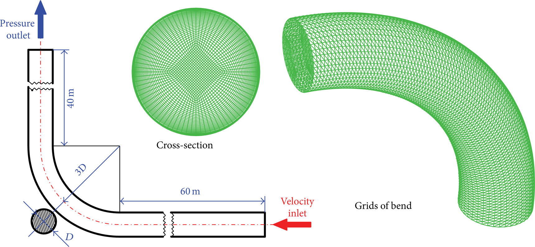
Schematic of the sand discharge pipe and mesh model of the key calculative domain (bend).

Due to the fact that the change of the temperature in sand discharge pipe is very little, the total temperature is fixed at 300 K in simulations. Density of nitrogen is a variable corresponding to pressure for its compressibility. In standard state (273.15 K and 101.325 KPa), its density is defined as 1.138 kg/m³. The viscosity of nitrogen seemed constant as 1.663 × 10⁻⁵ Pa·s. Sand particles are treated as spherical particles with density of 2800 kg/m³. For analyzing the effect of particle diameter, three different particle sizes, 0.5 mm, 0.75 mm, and 1 mm, are chosen in simulations. The material of the discharge pipe is steel, whose density, Young's modulus and damping ratio of steel are defined as 7850 kg/m³, 196 GPa, and 0.05, respectively.

3. Governing Equations and Numerical Method

3.1. Governing Equations

An Eulerian-Lagrangian approach is applied to analyze the continuum phase and particle tracking for sand particles, in which, compressible nitrogen flow is treated as the continuum phase evaluated by the RANS equations based on the Eulerian approach, while sand particles are treated as spherical particles added into continuum phase flow field as discrete phase, which are captured by DPM based on the Lagrangian approach.

The RANS equations used to solve the continuum phase include continuity and momentum equations and are written as follows [16 –18]:

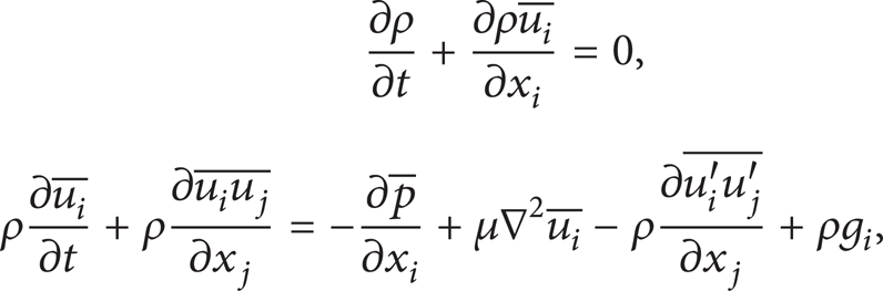
\begin{matrix} \frac{\partial ρ}{\partial t} + \frac{\partial ρ \overset{—}{u_{i}}}{\partial x_{i}} = 0, \\ ρ \frac{\partial \overset{—}{u_{i}}}{\partial t} + ρ \frac{\partial \overset{—}{u_{i}} \overset{—}{u_{j}}}{\partial x_{j}} = - \frac{\partial \overset{—}{p}}{\partial x_{i}} + μ \nabla^{2} \overset{—}{u_{i}} - ρ \frac{\partial \overset{—}{u_{i}^{'} u_{j}^{'}}}{\partial x_{j}} + ρ g_{i}, \end{matrix}

(1)

where u_i represents instantaneous velocity component in i direction, while u_i′ is fluctuation velocity component in i direction, x_i is space coordinate in i direction, g_i is gravitational acceleration in i direction, t is time, p is pressure, and ρ and μ are density and viscosity, respectively.

Since the Reynolds number ranges from 3.038 × 10⁵ to 1.044 × 10⁶ in the calculations, a realizable k-ε turbulence model [19 –23] is employed to close the flow governing equations and describe the turbulent properties:

\begin{matrix} \frac{\partial (ρ k)}{\partial t} + \frac{\partial (ρ k u_{i})}{\partial x_{i}} = \frac{\partial}{\partial x_{j}} [(μ + \frac{μ_{t}}{σ_{k}}) \frac{\partial k}{\partial x_{j}}] + G_{k} + G_{b} - ρ ε, \\ \frac{\partial (ρ ε)}{\partial t} + \frac{\partial (ρ ε u_{i})}{\partial x_{i}} = \frac{\partial}{\partial x_{j}} [(μ + \frac{μ_{t}}{σ_{ε}}) \frac{\partial ε}{\partial x_{j}}] + ρ C_{1} S ε - ρ C_{2} \frac{ε^{2}}{k + \sqrt{υ ε}} + C_{1 ε} (1 - C_{3 ε}) \frac{ε}{k} G_{b}, \end{matrix}

(2)

where

\begin{matrix} C_{1} = \max (0.43, \frac{η}{η + 5}), η = S \frac{k}{ε}, \\ S = {(2 S_{i j} \cdot S_{i j})}^{1 / 2}, S_{i j} = \frac{1}{2} (\frac{\partial u_{i}}{\partial x_{j}} + \frac{\partial u_{j}}{\partial x_{i}}), \\ G_{k} = - ρ \overset{—}{u_{i}^{'} u_{j}^{'}} \frac{\partial u_{j}}{\partial x_{i}}, G_{b} = - g_{i} \frac{μ_{t}}{P r_{t}} \frac{\partial ρ}{ρ \partial x_{i}}, μ_{t} = ρ C_{μ} \frac{k^{2}}{ε}, \end{matrix}

(3)

where k and ε represent turbulent kinetic energy and turbulent kinetic energy dissipation rate per unit mass, respectively, η is the relative strain parameter, S is the strain rate, G_k and G_b represent production term of turbulent kinetic energy due to the average velocity gradient and production term of turbulent kinetic energy due to lift, respectively, υ is kinematic viscosity of fluid, μ_t is turbulent viscosity, Pr_t is Prandtl number taken as 0.85, C_μ, C_1ε, C₂, and C_3ε are empirical model constants taken as 0.09, 1.44, 1.9, and 0.9, respectively, and σ_t and σ_ε are turbulent Prandtl numbers taken as 1.0 and 1.2, respectively.

After the flow field of the continuum phase being obtained by solving the aforementioned equations, a particle motion equation is used to describe the turbulent properties of the discrete phase, including the trajectory of particles, the attack angle, and velocity perturbation [24, 25]. This particle motion equation is called the DPM model:

\frac{d u_{s}}{d t} = \frac{C_{D} R e_{s}}{24 τ_{t}} (u - u_{s}) + \frac{g (ρ_{s} - ρ)}{ρ_{s}} + 0.5 \frac{ρ}{ρ_{s}} \frac{d (u - u_{s})}{d t},

(4)

where

\begin{matrix} τ_{t} = \frac{ρ_{s} d_{s}^{2}}{18 μ}, R e_{s} = \frac{ρ d_{s} | u_{s} - u |}{μ}, \\ C_{D} = \frac{24}{R e_{s}} (1 + b_{1} R e_{s}^{b_{2}}) + \frac{b_{3} R e_{s}}{b_{4} + R e_{s}}, \end{matrix}

(5)

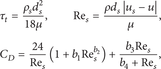
where u_s represents velocity of solid particle, C_D is drag coefficient, Re_s is particle equivalent Reynolds number, ρ_s is density of solid particle, τ_t is particle relaxation time, and b₁, b₂, b₃, and b₄ are empirical constants taken as 0.186, 0.653, 0.437 and 7178.741, respectively.

Then the erosion rate can be determined by the mass transfer rate of magnetite on the metal surface, which takes the following form [26]:

e = \sum_{s = 1}^{N_{s}} \frac{1.8 \times 1 0^{- 9} M_{s}}{A},

(6)

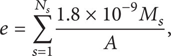
where e is the erosion rate, M_s and N_s represent the mass rate and number of particles, respectively, and A is the projected area of particles in wall.

3.2. Numerical Method

The finite volume method (FVM) is used to discretize the aforementioned equations. All the calculations are carried out using a commercial software package FLUENT 14.0, in which DPM is adopted to capture the discrete phase based on the Lagrangian approach. Patankar's well-known SIMPLE algorithm [27] is employed to solve the pressure-velocity coupling. And second-order upwind scheme and second-order central-differencing scheme are used for convective terms and diffusion terms, respectively, in order to ensure the accuracy of calculation. The convergent criteria for all calculations are set as that the residual in the control volume for each equation is smaller than 10⁻⁵.

3.3. Computational Mesh

ICEM CFD mesh-generator is employed to perform the geometry generation and meshing. As shown in Figure 1, the computational domain is divided into five blocks and progressive mesh is used to capture the near-wall flow properties. In order to control the grid distribution and computational stability, each block is discretized with hexahedral cells. A suitable grid density is reached by repeating computations until a satisfactory independent grid is found. For example, the number of hexahedral cells for discharge pipe with the outer diameter of 168 mm and bend curvature of 3 is 2245684 at last.

3.4. Boundary Conditions

At the inlet, the velocities of nitrogen and sand particles are defined as the same value and uniform distribution. After traveling a certain distance in the front straight pipe, they will form a fully developed flow. In order to examine the effects of inlet condition, the inlet rates of nitrogen and sand particles are taken as 30 m/s, 40 m/s, and 50 m/s in comparing cases, and the sandy volume fraction in inlet is set to 3%, 6%, or 9%.

Pressure outlet boundary condition is used for the outlet of the computational domain. And the value is defined as 0 Pa in order to facilitate comparative analysis. Finally, no slip boundary condition is imposed on the discharge pipe inner wall.

The information of simulation cases is listed in Table 1, in which inlet rate, pipe outer diameter, bend curvature, inlet sandy volume fraction, and particle diameter are the five variables.

Table 1:

Simulation cases.

Case	Inlet rate (m/s)	Pipe outer diameter (mm)	Bend curvature	Inlet sandy volume fraction (%)	Particle diameter (mm)

1	30	273	3	6	1
2	40	273	3	6	1
3	50	273	3	6	1
4	40	168	3	6	1
5	40	325	3	6	1
6	40	273	2	6	1
7	40	273	4	6	1
8	40	273	3	3	1
9	40	273	3	9	1
10	40	273	3	6	0.75
11	40	273	3	6	0.5

4. Numerical Results and Discussion

4.1. Effect of Inlet Velocity and Simulation Validation

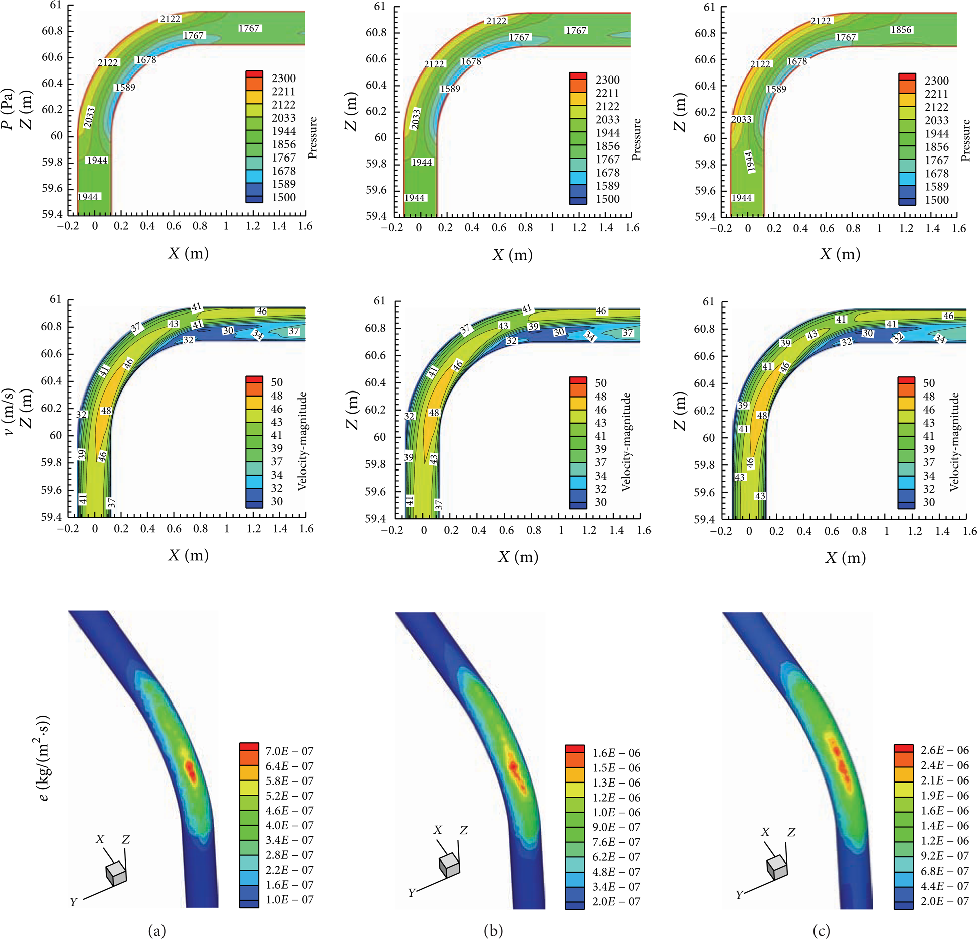
We focus on the flow properties and flow erosion in the bend, since it is the main failure part of sand discharge pipe. Figure 2 shows the pressure and velocity distribution of cuttings-carrying flow at the longitudinal cross-section in the bends at different inlet velocities. To have a better understanding of flow field in the bend, the contours and values are marked in the figure.

Figure 2:

Static pressure distribution and velocity distribution at the middle plane of bend and erosion rate distribution at the bend wall at different inlet velocities: (a) inlet velocity = 30 m/s; (b) inlet velocity = 40 m/s; (c) inlet velocity = 50 m/s.

It is seen that the flow field is disturbed when flow enters the bend. There is a significant pressure drop for gas-solid flow through the elbow. The pressure is uniform across the flow as the fluid just flows into the bend. However, its distribution changes dramatically in the elbow, showing an obvious pressure gradient along the direction of the radius of bend curvature. It can be observed that the highest pressure is along the extrados farthest from the center of curvature while the lowest pressure is along the intrados nearest to the center of curvature. This is mainly caused by flow countering the centrifugal force formed in the elbow when flow direction is forced to turn. This pressure gradient established in the bend has well-known effects on the flow, which produces a secondary flow. At an inlet flow rate of 30 m/s, the cross-stream pressure gradient is 924.9 Pa/m, about three-tenths of the pressure gradient for an inlet flow rate of 50 m/s. It means that the cross-stream flow is more intense at high speed, bringing about greater impinging on elbow wall. The total pressure drop for fast flow (inlet flow rate = 50 m/s) passing through the elbow is about 1.43 times larger than that for slow flow (inlet flow rate = 30 m/s).

As shown in Figure 2, the curvature of the bend causes non-uniform velocity distributions around the bend. The flow rate along the extrados decreases due to the effect of an adverse streamwise pressure gradient, while the flow rate along the intrados increases. The high cross-stream velocity gradient near the outer wall of the bend is worth noting. It indicates that more kinetic energy transfer and release occurs in this region. The higher the inlet rate is, the greater the velocity gradient is. Therefore, particles' impinging on the bend outer wall is greater for high-speed flow. It is verified from the erosion rate distributions shown in Figure 2.

It can be seen that the erosion rate on the outer wall is much larger than that on the inner wall, and the maximum erosion rate is located at 30–50° of the outer wall. The particles along with high-speed flow have a high inertia. Therefore, the severity of erosion is enhanced with the increase in inlet rate, which is not only reflected in the value of the erosion rate but also reflected in the range of severe erosion area. The maximum value of erosion rate in slow flow (inlet flow rate = 30 m/s), 1.2 × 10⁻⁶ kg/(m²·s), is just four tenths of that in fast flow (inlet flow rate = 50 m/s). And the most severe erosion area at the outer wall increases five times as inlet rate increases from 30 m/s to 50 m/s. Since the erosion rate increases exponentially with the increase in flow rate, appropriate operation parameters should be taken to control the flow rate in the discharge pipe below a limited value.

To validate the numerical model in this study, erosion rate on the bend wall is tested. After bends serviced a period of time under the same working conditions as case 1, case 2, and case 3, we have removed them and measured the depth of erosion pits on the elbows' walls. Then we obtained the maximum erosion rate. These measured data, shown in Figure 3, are compared with the simulation results as presented previously. It can be found that the numerical predicted erosion rates are consistent with the measured results. The maximum error of simulation results is under 8.5%. And the calculated results are slightly larger than the measured values. Using the predicted erosion rate is safer. Therefore, this numerical method is sufficiently accurate to predict the erosion rate.

Figure 3:

Comparison between simulation results and measurement values.

4.2. Effect of Pipe Diameter

Figure 4 presents the flow pattern in the bends with different pipe diameters. The total pressure drop of flow passing through large diameter bend is smaller than that in small diameter bend. The pressure drop decreases from 1000 Pa to 800 Pa as the diameter of the pipe increases from 168 mm to 325 mm. The similar change trend is found in the cross-stream pressure gradient, which is 3006.8 Pa/m in the bend with the diameter of 168 mm, 1.43 times larger than that for the one diameter of 273 mm and 1.72 times larger than that for with the diameter of 325 mm. The velocity distributions along the stream are similar in different-diameter bends, while the cross-stream velocity gradient near the outer wall of the bend increases with the reduction in diameter. This velocity gradient is 263.5 s⁻¹ in the bend with the diameter of 168 mm, which is about 2.32 times larger than that in the bend with the diameter of 325 mm.

Figure 4:

Static pressure distribution and velocity distribution at the middle plane of bend and erosion rate distribution at the bend wall at different outer diameters: (a) outer diameter = 168 mm; (b) outer diameter = 273 mm; (c) outer diameter = 325 mm.

It can be seen from Figure 4 that decreasing of pipe diameter leads to the rise in the erosion rate. The maximum erosion rate of approximately 3.0 × 10⁻⁶ kg/(m²·s) is presented at the small-diameter bend (out diameter = 168 mm). However, the most severe erosion area is limited comparing to that in the big-diameter bend. Under the same inlet rate condition, greater mass flow rate in the big-diameter pipe could be a major cause for the large area of erosion. Another reason for it can be attributed to the large frontal area in the big bend. But the erosion problems in the small bend should be paid more attention, because the concentrated impinging on the small area of the bend wall usually leads to perforation failure, which is prone to happen earlier.

4.3. Effect of Bend Curvature

In Figure 5, it depicts the flow field at the middle plane of bend and erosion rate distribution at the bend wall at different bend curvatures. There is an obvious cross-stream pressure gradient in the small-curvature bend, which is 2458.5 Pa/m in the bend with R/D of 2, about 2.34 times greater than that in the bend with R/D of 4. Due to the rapid turn in the small-curvature bend, the cross-stream velocity gradient near the outer wall of the bend is larger and twisted velocity contours are present near the inner wall just downstream from 45°.

Figure 5:

Static pressure distribution and velocity distribution at the middle plane of bend and erosion rate distribution at the bend wall at different bend curvatures: (a) bend curvature (R/D) = 2; (b) bend curvature (R/D) = 3; (c) bend curvature (R/D) = 4.

Under the action of this flow field, the sand particles flow along the nitrogen flow and impinge on the wall of the bend resulting in significant erosion. The maximum erosion rate of 9.0 × 10⁻⁶ kg/(m²·s) presenting in the bend with R/D of 2 is 7.5 times greater than that in the bend with R/D of 4. And the most severe erosion area for R/D of 2 is mainly located at 35–45° of the outer wall, while the erosion area for R/D of 4 extends from 30° to 85° of the bend outer wall. Therefore, perforation may be the main failure of the small-curvature bend, while crack may be the main failure form in the large-curvature bend.

4.4. Effect of Sand Concentration

The process of drilling a deep well usually encounters different strata, bringing about different sand concentrations and sand sizes. Thus, a number of simulations have been performed by varying the inlet sandy volume fraction or sand particle diameter while other variables are fixed at their base values. Figure 6 gives the pressure and velocity distribution and erosion rate profile at different inlet sandy volume fractions. The differences of pressure and velocity contours are not obvious for different inlet sandy volume fractions. But the erosion rate distribution has an obvious difference. For small inlet sandy volume fraction, the reduction in the amount of particles weakens the erosion-dominated regime significantly. The maximum erosion rate in case 8 is just 27% of that in case 9. Therefore, we cannot ignore the change in sandy volume fraction. In practice, the particle concentration should be monitored in real time to conduct proper adjustments.

Figure 6:

Static pressure distribution and velocity distribution at the middle plane of bend and erosion rate distribution at the bend wall at different inlet sandy volume fractions: (a) inlet sandy volume fraction = 3%; (b) inlet sandy volume fraction = 6%; (c) inlet sandy volume fraction = 9%.

4.5. Effect of Sandy Particle Diameter

Figure 7 displays the flow field and erosion rate distribution at different sand sizes. Since the inlet sandy volume fraction is fixed at 6%, the reduction of particle diameter produces the increase in the number of particles. However, the differences of pressure and velocity contours are also not obvious due to the limited total amount of solid particles in the nitrogen flow. It is observed that with decreasing particle diameter the erosion is weakened. The maximum erosion rate decreases from 1.6 × 10⁻⁶ kg/(m²·s) to 3.0 × 10⁻⁷ kg/(m²·s) as particle diameter decreases from 1 mm to 0.5 mm. It can be explained that with the same rate particles of big diameter have more impinging energy than small particles. Another reason is that the centripetal force of the bigger particle is larger than that of the small one. Therefore, a proper drill bit which can cut rocks into small particles should be applied in actual drilling in order to weaken the flow erosion in the discharge pipe.

Figure 7:

Static pressure distribution and velocity distribution at the middle plane of bend and erosion rate distribution at the bend wall at different sandy particle diameters: (a) particle diameter = 1 mm; (b) particle diameter = 0.75 mm; (c) particle diameter = 0.5 mm.

5. Conclusions

A numerical method, for examining the flow erosion on sand discharge pipe in nitrogen drilling, by finite volume simulation combined with DPM is proposed. Effects of flow parameters such as inlet velocity, sandy volume fraction, and particle diameter and structure parameters such as pipe diameter and bend curvature are analyzed by conducting a series of simulations. Based on the numerical results, the following conclusions can be drawn.

Flow field changes dramatically in the elbow, showing an obvious cross-stream pressure gradient and a high cross-stream velocity gradient near the outer wall of the elbow. Inlet rate, pipe diameter, and bend curvature affect the flow field significantly, while small changes in sand concentration and particle diameter have little influence on flow.

Erosion rate is sensitive to inlet velocity, pipe diameter, bend curvature, sandy volume fraction, and particle diameter. The smaller the pipe diameter is or the smaller the bend curvature is, the more serious the erosion is. However, erosion can be weakened by reducing the flow rate or reducing the sandy concentration and particle size.

The detailed results presented in this work provide useful information for the design engineer to overcome the flow erosion on sand discharge pipe. These references have been used to guide actual nitrogen drilling in Sichuan.

Footnotes

Acknowledgments

Research work was supported by Open Fund (no. PLN1210) of State Key Laboratory of Oil and Gas Reservoir Geology and Exploitation (Southwest Petroleum University) and the National Natural Science Foundation of China (no. 51274170). Without the support, this work would not have been possible.

References

Wang

Y. M.

Y. J.

, and Zheng

M. T.

, “Optimized design of clearance pipeline for gas drilling,” Natural Gas Exploration and Development, vol. 31, pp. 45–59, 2008.

Liu

G. H.

, and Wang

X. Z.

, “Open loop field test for nitrogen circulation drilling,” Oil Drilling & Production Technology, vol. 32, pp. 9–12, 2010.

Zhang

F. Z.

, Complex Drilling Technology, China Petroleum Industry Press, Beijing, China, 2006.

Zou

G. G.

Lin

F. Q.

Xiong

, and Yang

D. C.

, “Practice of gas drilling in piedmont structure of Tarim oilfield,” Drilling & Production Technology, vol. 33, pp. 22–24, 2010.

Zhu

H.-J.

Lin

Y.-H.

Zeng

D.-Z.

, and Yan

R.-T.

, “Simulations of flow induced corrosion in api drillpipe connector,” Journal of Hydrodynamics, vol. 23, no. 6, pp. 784–791, 2011.

Njobuenwu

D. O.

and Fairweather

, “Modelling of pipe bend erosion by dilute particle suspensions,” Computers and Chemical Engineering, vol. 42, pp. 235–247, 2012.

Stack

M. M.

and Abdelrahman

S. M.

, “A CFD model of particle concentration effects on erosion-corrosion of Fe in aqueous conditions,” Wear, vol. 273, no. 1, pp. 38–42, 2011.

Tan

Y. Q.

Zhang

Yang

D. M.

Jiang

S. Q.

Song

J. H.

, and Sheng

, “Numerical simulation of concrete pumping process and investigation of wear mechanism of the piping wall,” Tribology International, vol. 46, pp. 137–144, 2012.

Tang

Yang

Zheng

J. Y.

, “Erosion-corrosion failure of REAC pipes under multiphase flow,” Frontiers of Energy and Power Engineering in China, vol. 3, no. 4, pp. 389–395, 2009.

10.

Kuan

Yang

, and Schwarz

M. P.

, “Dilute gas-solid two-phase flows in a curved 90° duct bend CFD simulation with experimental validation,” Chemical Engineering Science, vol. 62, pp. 2068–2088, 2007.

11.

Chen

X. H.

Mclaury

B. S.

, and Shirazi

S. A.

, “Numerical and experimental investigation of the relative erosion severity between plugged tees and elbows in dilute gas/solid two-phase flow,” Wear, vol. 261, no. 7–8, pp. 715–729, 2006.

12.

Jiang

, and Sun

, “Experimental study and numerical investigation of particle penetration and deposition in 90° bent ventilation ducts,” Building and Environment, vol. 46, no. 11, pp. 2195–2202, 2011.

13.

Zhang

Tan

Y. Q.

Yang

D. M.

Trias

F. X.

, and Jiang

S. Q.

, “Numerical investigation of the location of maximum erosive wear damage in elbow: effect of slurry velocity, bend orientation and angle of elbow,” Powder Technology, vol. 217, pp. 467–476, 2012.

14.

Ferng

Y. M.

and Lin

B. H.

, “Predicting the wall thinning engendered by erosion-corrosion using CFD methodology,” Nuclear Engineering and Design, vol. 240, no. 10, pp. 2836–2841, 2010.

15.

Tang

Yang

Zheng

J. Y.

, “Failure analysis and prediction of pipes due to the interaction between multiphase flow and structure,” Engineering Failure Analysis, vol. 16, no. 5, pp. 1749–1756, 2009.

16.

Alfonsi

, “Reynolds-averaged Navier-Stokes equations for turbulence modeling,” Applied Mechanics Reviews, vol. 62, no. 4, Article ID 040802, 20 pages, 2009.

17.

Hinze

J. O.

, Turbulence, McGraw Hill, New York, NY, USA, 1975.

18.

Frisch

, Turbulence, Cambridge University Press, London, UK, 1995.

19.

Karim

V. M.

and Bart

, “Application of two buoyancy-modified k-∊ turbulence models to different types of buoyant plumes,” Fire Safety Journal, vol. 41, no. 2, pp. 122–138, 2006.

20.

Chintala

and Subramanian

K. A.

, “A CFD (computational fluid dynamics) study for optimization of gas injector orientation for performance improvement of a dual-fuel diesel engine,” Energy, vol. 57, pp. 709–721, 2013.

21.

Mohammed

S. L.

Michael

Peter

, “CFD predictions of wake-stabilised jet flames in a cross-flow,” Energy, vol. 57, pp. 259–269, 2013.

22.

Rohdin

and Moshfegh

, “Numerical predictions of indoor climate in large industrial premises. A comparison between different k-∊ models supported by field measurements,” Building and Environment, vol. 42, no. 11, pp. 3872–3882, 2007.

23.

M. K.

Utomo

Woo

J. S.

Lee

Y. H.

Jeong

H. M.

, and Chung

H. S.

, “CFD investigation on the flow structure inside thermo vapor compressor,” Energy, vol. 35, no. 6, pp. 2694–2702, 2010.

24.

Sun

Lin

J.-Z.

F.-L.

, and Chen

Y.-M.

, “Effect of non-spherical particles on the fluid turbulence in a particulate pipe flow,” Journal of Hydrodynamics, vol. 16, no. 6, pp. 721–729, 2004.

25.

Dickenson

J. A.

and Sansalone

J. J.

, “Discrete phase model representation of Particulate Matter (PM) for simulating PM separation by hydrodynamic unit operations,” Environmental Science and Technology, vol. 43, no. 21, pp. 8220–8226, 2009.

26.

Zhu

H. J.

Lin

Y. H.

Zeng

D. Z.

Zhou

Xie

, and Wu

Y. P.

, “Numerical analysis of flow erosion on drill pipe in gas drilling,” Engineering Failure Analysis, vol. 22, pp. 83–91, 2012.

27.

Patankar

S. V.

, Numerical Heat Transfer and Fluid Flow, McGraw-Hill, New York, NY, USA, 1980.

Numerical Analysis of Flow Erosion on Sand Discharge Pipe in Nitrogen Drilling

Abstract

1. Introduction

2. Problem Description

3. Governing Equations and Numerical Method

3.1. Governing Equations

3.2. Numerical Method

3.3. Computational Mesh

3.4. Boundary Conditions

4. Numerical Results and Discussion

4.1. Effect of Inlet Velocity and Simulation Validation

4.2. Effect of Pipe Diameter

4.3. Effect of Bend Curvature

4.4. Effect of Sand Concentration

4.5. Effect of Sandy Particle Diameter

5. Conclusions

Footnotes

Acknowledgments

References