Sage Journals: Discover world-class research

Abstract

Both a numerical and an analytical models were developed to simulate temperature profiles in continuous laminar pipe flow during microwave heating. Fully developed velocity and thermally developing conditions were assumed. The numerical solution was obtained by first solving Maxwell equations and then by coupling them with the energy balance for the flowing fluid. On the other hand, the same problem was solved analytically under the simplifying assumption foreseeing uniform heat generation inside the pipe. With the aim of reducing computational efforts, numerical and analytical results were compared in order to investigate conditions for which the two models allowed to recover the same temperature patterns. Thus, it has been shown that suitable conditions can be found for which the simplified analytical model can lead to an easy way to predict the heat transfer through the pipe.

1. Introduction

Nowadays, it is widely accepted that using microwaves (MWs) as a source of energy turns out into a viable alternative for high-temperature/short-time processing featuring several industrial food treatments. In fact, volumetric heating due to microwaves leads to higher heat transfer rates and hence to shorter processing times than conventional processes. These features are appealing since reduced thermal transients as well as the absence of high-temperature surfaces in contact with the foods could ensure both a lower stress for the food under processing [1] and improved food quality; in particular, a better conservation of vitamins during pasteurization processes than traditional heating is usually observed [2, 3]. Additional benefits can be related to continuous flow MW heating systems since they enable in realizing increased productivity, easier clean up and automation with respect to standard batch ones [4]; space saving and simplified piping when compared with traditional heat plants are expected too. Therefore, increasing demand for industrial applications is actually taking place. In this framework, it is worth noting that

since available energy densities are typically smaller than the ones achievable by conventional techniques, laminar flow conditions are often realized in order to realize acceptable temperature increases [5, 6];

wishing to enhance heat transfer rates, laminar flow is not disadvantageous since heat transfer is no more driven by wall conditions; therefore, reduced heat transfer coefficients could even be helpful, the walls being warmer than the external air.

On the other hand, the complexity due to the electromagnetic (EM) field prediction and, in turn, to the related heat generation term is a major obstacle in designing industrial applications for microwave food heating. In fact, thermal response is to be correlated to relative load and system configurations and to thermal and dielectric properties of the material as a function of chemical composition, temperature, and frequency [7 –12]. Moreover, difficulties are experienced in measuring and/or controlling temperature in the cavity because traditional probes fail and highly uneven temperature patterns are usually realized [13, 14]. In addition, adequate experimentation may be impractical, as a large number of tests are usually required to obtain representative results [15, 16]. Further difficulties in recovering theoretical solutions have to be accounted for when considering continuous pipe flow: solving simultaneously high-frequency electromagnetism, heat transfer, and fluid-flow problems requires high-computation time, programming, and numerical analysis skills [17]. In addition, numerical discretization in time and space leads to variations in numerical phase velocities which in turn can bring cumulative errors (“grid dispersion” phenomenon). Therefore, special care has to be paid in mesh generation. Since common criteria (e.g., the Nyquist-Shannon sampling theorem) may fail [18, 19], in Section 3 a more restrictive criterion, still based on simplified assumptions, is proposed.

Almost recently, the numerical approach, in view of several simplifying assumptions, allowed a satisfying description of the coupled thermal-EM problems and an accurate identification of the effects which the operating parameters have on the process at hand [9, 12, 17, 18, 20 –23]. In addition, numerical techniques represent an effective way for solving more complex problems (e.g., [24]) in which temperature-dependent dielectric permittivity as well as non-Newtonian liquids carrying food subjected to MW heating may be taken into account. In the above framework, alternative procedures based on approximate methods can be found; the latter are essentially based on attempting a suitable simplified modelling for the generation term in the energy equation. The latter procedure is acceptable by considering that in the field of food engineering it is often desired to control the thermal effect of microwave heating, while detailed knowledge of EM field behaviour is unnecessary. Of course, approximate theoretical approaches can be helpful in pointing out the overall thermal behaviour and the main parameters controlling the problem at hand and their influence on the thermal response [5] before realizing an experimental validation. Meanwhile, costs and the outlined problems related to experimental procedures are avoided.

As a consequence of the foregoing discussion, aiming to a faster and easier model for continuous microwave heating of liquids, the possibility of recovering the fluid thermal behaviour by an analytical solution is investigated in the present paper; uniform heat generation inside the pipe is assumed, retaining the proper average value. This presumption is suggested by supposing that

temperature patterns for the flowing fluid are determined by the volume-averaged heat generation, rather than by its local values, as much as the fluid speed increases;

the illuminated cavity volume is sufficiently large with respect to the applicator pipe to behave as a reverberating chamber, thus reducing uneven EM-field patterns.

Conditions, if any, are then searched for which the above assumptions become effective, thus leading to convergence between the simplified analytical problem and the reference-numerical solution for the temperature field.

To address the problem, a three-dimensional numerical model was first developed to predict the distribution of the EM field in water continuously flowing in a circular duct subjected to microwave heating. The Maxwell's equations were solved using the finite element method (FEM) in the frequency domain to describe the electromagnetic field configuration in the MW cavity.

As a first approach to the problem, water is described as an isotropic and homogeneous dielectric; its properties are assumed to be independent of temperature. Therefore, the momentum and the energy equations turn out to be one way coupled with Maxwell's equations and are then solved both numerically and analytically; the developing temperature field for an incompressible laminar duct flow subjected to heat generation is considered. The latter is sought as the effective one arising from the solution of the electromagnetic problem at hand, whereas its average value over the water volume is assumed with reference to the analytical solution.

2. Basic Equations

2.1. MW System Description

A general-purpose pilot plant producing microwaves by a magnetron rated at 2 kW and emitting at a frequency of 2.45 GHz is available to the heat transfer laboratory, at the University of Salerno, Figure 1; it will be used for future development of the present work, aiming to validate the results herein presented. Thus, the following models are referred to such an experimental setup. The insulated metallic cubic chamber houses one PTFE applicator pipe; the pipe is embedded in a box made by a closed-cell polymer foam. The matrix foam was proven to be transparent to microwaves at 2.45 GHz. As stated in the introduction, the cavity is designed such that its volume is much greater than the applicator pipe, aiming to approximate a reverberant chamber behaviour.

Figure 1:

Sketch of the available setup.

2.2. Electromagnetic Problem

Three-dimensional numerical modelling of continuous flow microwave heating was carried out by employing the commercial code COMSOL v4.3 [25]. The latter can provide coupling of three physical phenomena, electromagnetism, fluid, and energy flow. First, the Maxwell's equations are solved by means of the finite element method (FEM) [26] using unstructured tetrahedral grid cells; then, the electric field distribution $\underline{E}$ in the microwave cavity, both for air and for the applicator pipe carrying the fluid under process, is determined by imposing

\begin{matrix} \nabla \times (\frac{1}{μ_{r}} \nabla \times \underline{E}) - k_{0}^{2} (ε_{r} - \frac{i σ}{ω ε_{0}}) \underline{E} = \underline{0}, \end{matrix}

(1)

where $\underline{E}$ is the electric field intensity, ε_r is the relative permittivity, ω is the angular wave frequency, μ_r is the relative permeability of the material, k₀ is the wavenumber in vacuum, and σ is the electric conductivity. Air and the PTFE applicator tube were both supposed to be completely transparent to microwaves. Assuming negligible resistive material losses, boundary conditions for the radio frequency module included perfect electric conductors walls, that is, $\underline{n}$ × $\underline{E}$ = 0, for the waveguide and the cavity, being $\underline{n}$ the local normal vector. At the port, an amount of 2 kW EM power, 2450 MHz frequency, was supplied through a rectangular TE10 mode waveguide (WR 340).

Continuity boundary condition was set by default for all the interfaces between the confining domains, that is, the pipe, the cavity, and the waveguide. Formally, such condition may be expressed as

\begin{matrix} \underline{n} \times ({\underline{E}}_{i} - {\underline{E}}_{j}) = \underline{0}, \end{matrix}

(2)

i and j being the domains sharing the interface at hand. Scattering boundary conditions were applied at the inlet and the outlet of the pipe to make the pipe's ends transparent to incoming waves, avoiding that undesired reflected waves travel inward [15].

Total volumetric power generation due to microwaves is calculated by

\begin{matrix} U_{gen} = 2 π ε_{0} ε^{′′} f {| \underline{E} |}^{2}, \end{matrix}

(3)

where ε₀ is the free-space permittivity and ε” is the relative dielectric loss of the material.

Only one-half of the problem was modelled due to the symmetric geometry and load conditions around the XY plane crossing vertically the oven, the waveguide, and the pipe, see Figure 1, right side. The condition of perfect magnetic conductor was applied for the surfaces lying on the symmetry plane:

\begin{matrix} \underline{n} \times \underline{H} = \underline{0}, \end{matrix}

(4)

$\underline{H}$ being the magnetic field, which has to be therefore parallel to the local normal vector $\underline{n}$ on the XY plane.

2.3. Heat Transfer Problem

The power-generation term realizes the coupling of the EM field with the energy balance equation where it represents the “heat source” term. Convective terms in the energy equation require specifying velocity components, which are evaluated considering fully developed velocity profiles. Thus, for Newtonian-incompressible fluid in laminar motion, the Navier-Stokes equations yield the well-known axial Poiseille velocity profile U(R) with no radial component (V = 0), being the radius R ∈ (0, D_i/2) and D_i the internal pipe diameter.

In view of the above assumptions and considering constant properties, the energy balance reduces to

\begin{matrix} ρ c_{p} U \frac{\partial T}{\partial X} = k \nabla^{2} T + U_{gen}, \end{matrix}

(5)

where T is the temperature, ρ is the fluid density, c_p is the specific heat, k is the thermal conductivity, X is the axial coordinate, andU_gen is the specific heat generation.

The PTFE tube carrying the fluid exposed to microwave irradiation is considered thermally meaningless. The inlet temperature is set to 10°C, while the remaining boundaries are assumed as adiabatic. Fixed average velocities (namely, U_av = 0.02, 0.04, 0.08, 0.16 m/s) were chosen.

After processing the numerical model, the average spatial value for heat generation was obtained; then, it was used as a source term for feeding the analytical solution. Consider that, in practice, such parameter can be measured by calorimetric methods, avoiding numerical calculations, therefore enabling the application of the analytical model with ease.

3. Numerical Model

A numerical model was developed in COMSOL 4.3 [25] to predict temperature patterns in the fluid continuously heated in a multimode microwave illuminated chamber. The radio frequency package, developed for the analysis of propagating electromagnetic waves, was one way coupled with the heat transfer module to solve the energy balance equation in the thermally developing region. The fluid dynamics problem was considered laminar and fully developed, and thus, velocity profiles were assumed to be known and parabolic.

3.1. Geometry Building

The assumed configuration for the system at hand is sketched in Figure 1, left side. The pipe carrying the fluid to be heated was 6 mm internal diameter and 0.90 m long. The three-dimensional setup was generated in SolidWorks, providing symmetrical geometry and load conditions about the XY symmetry plane. Such a choice was performed having in mind to suitably reduce both computational burdens and mesh size while preserving the main aim of the paper that is to compare the simplified analytical solution with the numerical one. In particular, a cubic cavity chamber (side length, L = 0.9 m) and a standard WR340 waveguide were assumed.

3.2. Mesh Generation

The available computational domain, reduced by one half as previously specified, was discretized using unstructured tetrahedral grid elements. Special care was devoted in choosing their size, as numerical dispersion may result in the presence of a numerical phase velocity error in the solution. Grid dispersion may appear in numerical methods such as finite-element or finite-difference methods. The phenomenon should not be underestimated because such propagating errors are cumulative, yielding unacceptable solution once propagating waves travel over considerable distances. Common sampling criteria, such as Nyquist's, may fail under certain circumstances.

For the sake of clarity, the simple case of the homogeneous lossless 1D Maxwell wave equation travelling in time t over the x-axis direction is considered

\begin{matrix} \frac{\partial^{2} E}{\partial t^{2}} = c^{2} \frac{\partial^{2} E}{\partial X^{2}}, \end{matrix}

(6)

$c = 1 / \sqrt{ε μ}$ being the wave speed in the medium, ε = ε_rε₀ the absolute electrical permittivity, and μ = μ_rμ₀ the absolute magnetic permeability. Free space permittivity and permeability are known to be ε₀ = 8.854 10⁻¹² F/m and μ₀ = 4π10⁻⁷ H/m, respectively. This equation is known to be dispersionless. In fact, the general solution expressed in phasor form

\begin{matrix} E (X, t) = e^{j (ω t - k X)}, j = \sqrt{- 1} \end{matrix}

(7)

admits as continuous dispersion relationship the following equation

\begin{matrix} k = \pm \frac{ω}{c}, \end{matrix}

(8)

the wavenumber k being the function of the angular frequency ω. The latter arises by introducing the second temporal and spatial derivatives of (7) in (6), which gives for the wave phase velocity

\begin{matrix} v_{p} ≝ \frac{ω}{k} = \pm c, \end{matrix}

(9)

a quantity independent from the linear f or angular frequency ω. Such nondependence cannot be stated when considering a numerical discretization of (6). Let us consider its finite difference approximation of second-order accuracy in space and time (whose local coordinates are referred to the electric field subscripts and superscripts, resp.):

\begin{matrix} \frac{E_{p}^{m + 1} - 2 E_{p}^{m} + E_{p}^{m - 1}}{{(Δ t)}^{2}} + O [{(Δ t)}^{2}] = c^{2} {\frac{E_{p + 1}^{m} - 2 E_{p}^{m} + E_{p - 1}^{m}}{{(Δ X)}^{2}} + O [{(Δ X)}^{2}]} . \end{matrix}

(10)

Neglecting higher-order terms yields the explicit relation:

\begin{matrix} E_{p}^{m + 1} ≅ {(\frac{c Δ t}{Δ X})}^{2} (E_{p + 1}^{m} - 2 E_{p}^{m} + E_{p - 1}^{m}) + 2 E_{p}^{m} - E_{p}^{m - 1} . \end{matrix}

(11)

In analogy to (7), the general numerical solution in phasor form is introduced:

\begin{matrix} E_{p}^{m} ≅ {(\frac{c Δ t}{Δ X})}^{2} e^{j (ω m Δ t - \overset{—}{k} p Δ X)}, \end{matrix}

(12)

where $\bar{k} = {\bar{k}}_{re} + {j \bar{k}}_{im}$ is the complex wavenumber satisfying (12). The Courant number, CO = cΔt/ΔX, appearing in (12) must be lower than unity in order to guarantee a stable numerical solution. Such a stability limit is automatically checked by Comsol software each time step; hence, no more details concerning this aspect are here discussed. Numerical dispersion arises from the discrepancy between k and $\bar{k}$ wavenumbers. Again, introducing the second temporal and spatial derivatives of (12) in (11) yields the following identity for the complex wavenumber:

\begin{matrix} \overset{—}{k} = \frac{1}{Δ X} arccos {1 + {(\frac{Δ X}{c Δ t})}^{2} [\cos (ω Δ t) - 1]} . \end{matrix}

(13)

It can be noted that in this case the numerical wave phase velocity

\begin{matrix} {\overset{—}{v}}_{p} = \frac{ω}{\overset{—}{k}} \end{matrix}

(14)

turns out to be function of the angular frequency ω. Grid resolution directly affects (14). Considering the typical case corresponding to a wavelength $λ ≝ c / f = Δ X / 20$ and cΔt = ΔX/2 (i.e., a grid sampling density N_λ = λ/ΔX = 20 and CO = 0.5) yields the real equation:

\begin{matrix} {\overset{—}{v}}_{p} = 0.9968 c, \end{matrix}

(15)

that is, ε = 0.31% less than the wave speed c. Note that the error $ε = {\bar{v}}_{p} / c$ is lower than 1% for N_λ > 10 (horizontal line in Figure 2). Since it was considered a grid mesh resolution, spacing in the range 0.0107 ÷ 0.03 m and 0.002 ÷ 0.003 m for the vacuum and water, respectively, such a limit was strictly satisfied for the moving fluid (i.e., λ_water/ΔX_water > 30, λ_water being 0.09 m). The same limit is satisfied for the vacuum only where needed.

Figure 2:

Error $ε = (1 - {\bar{v}}_{p} / c) \cdot 100$ of ${\bar{v}}_{p}$ expressed as function of the grid sampling density N_λ, for Courant number CO = 0.5 (N_{λ, tr} = 3). Maximum absolute error can be estimated by setting c to the corresponding value for the fluid.

Extending to the general case, keeping N_λ and CO as variables, one can rewrite (13) as

\begin{matrix} \overset{—}{k} = \frac{1}{Δ X} arccos {1 + {(\frac{1}{CO})}^{2} [\cos (\frac{2 π CO}{N_{λ}}) - 1]} = \frac{1}{Δ X} arccos (ξ), \end{matrix}

(16)

in which ξ = – 1 marks the limit between real and complex values for $\bar{k}$ . Grid sampling resolution assumes correspondently the transitional value

\begin{matrix} N_{λ, tr} = \frac{2 π CO}{arccos (1 - 2 C O^{2})} . \end{matrix}

(17)

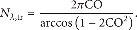
Limiting the analysis to the real values of (16), that is, N_λ > N_{λ, tr}, the relative error for ${\bar{v}}_{p}$ is shown in Figure 2, where N_{λ, tr} = 3 for the choice CO = 0.5.

As can be noted from the above discussion, assuming the maximum grid element size ΔX_max on the basis of the Nyquist criterion [19] (i.e., N_λ = 2) may turn in nonnegligible errors for the numerical wave phase velocity. Some studies (see, for instance, [18]) suggest that an acceptable criterion for the FEM solution of Maxwell's equations is to use six grids per wavelength; this is more stringent than Nyquist criterion, yet not always satisfying as reported in the above discussion.

4. The Analytical Model

The thermal model provides laminar-axisymmetric thermally developing flow of a Newtonian fluid with constant properties and negligible axial conduction. In such hypotheses, the dimensionless energy balanceequation and the boundary conditions in the thermal entrance region turn out to be

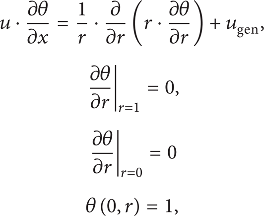
\begin{matrix} u \cdot \frac{\partial θ}{\partial x} = \frac{1}{r} \cdot \frac{\partial}{\partial r} (r \cdot \frac{\partial θ}{\partial r}) + u_{gen}, \\ {\frac{\partial θ}{\partial r} |}_{r = 1} = 0, \\ {\frac{\partial θ}{\partial r} |}_{r = 0} = 0 \\ θ (0, r) = 1, \end{matrix}

(18)

where θ = (T – T_s)/(T_i – T_s) is the dimensionless temperature, T_s and T_i being the temperature of the environment surrounding the tube and the inlet flow temperature, respectively; x = (4 · X)/(Pe · D_i) is the dimensionless axial coordinate; the Peclet number is defined as Pe = (U_av · D_i)/α, U_av being the mean fluid velocity and α the thermal diffusivity; r = (2 · R)/D_i is the dimensionless radial coordinate; u_gen = (U_gen · D_i²)/(4 · k · (T_i – T_s)) is the dimensionless heat generation, k being the thermal conductivity; u = 2 · (1 – r²) is the dimensionless radial velocity profile, u being U/U_av. The generation term has been obtained by evaluating the spatial average of the “electromagnetic power loss density” (W/m³) resulting from the EM problem.

The problem being linear, the thermal solution has been written as the sum of two partial solutions:

\begin{matrix} θ (x, r) = θ_{G} (x, r) + u_{gen} \cdot θ_{V} (x, r) . \end{matrix}

(19)

The θ_G(x, t) problem represents the solution of the extended Graetz problem featured by a nonhomogeneous equation at the inlet and adiabatic boundary condition at wall. On the other hand, the θ_V(x, t) problem takes into account the microwave heat dissipation and includes a non homogeneous differential equation. Thus, the two partial solutions have to satisfy the two distinct problems expressed in terms of θ_G(x, t) and θ_V(x, t), respectively. Details can be found in [5]. The θ_G problem is solved in closed form by the separation of variables method; thus, the structure of the solution is sought as follows:

\begin{matrix} \begin{matrix} θ_{G} (x, r) = \sum_{m = 1}^{M} c_{m} F_{m} (r) e^{- (λ_{m}^{2} / 2) \cdot x}, \\ F_{m} (r) = e^{- (r^{2} \cdot λ_{m} / 2)} \cdot Λ [\frac{1}{4} (- 2 + λ_{m}), r^{2} \cdot λ_{m}], \end{matrix} \end{matrix}

(20)

where F_m are the eigenfunctions, Λ being the orthonormal Laguerre polynomials and λ_m the related eigenvalues arising from the characteristic equation F_m′(1) = 0. Imposing the initial condition and considering the orthogonality of the eigenfunctions, the constants c_m were obtained.

The “θ_v” problem, featured by single nonhomogeneous equation, was solved assuming the solution as the sum of two partial solutions:

\begin{matrix} θ_{v} (x, r) = θ_{1} (r) + θ_{2} (x, r) . \end{matrix}

(21)

The “θ₁” problem holds the nonhomogeneus differential equation and represents the “x-stationary” solution. On the other hand, the “θ₂” problem turns out to be linear and homogenous with the exception of the “x-boundary” condition “θ₂(0, r) = – θ₁(r)”; then, it can be solved by the separation of variables method, recovering the same eigenfunctions and eigenvalues of the Graetz problem and retaining the same structure of (20):

\begin{matrix} θ_{2} (x, r) = \sum_{m = 1}^{M} b_{m} F_{m} (r) e^{- (λ_{m}^{2} / 2) \cdot x} . \end{matrix}

(22)

5. Results

5.1. Electromagnetic Power Generation and Cross-Section Spatial Power Density Profiles

The port input power was set to 2000 W. Due to the high impedance mismatch, as the available cavity was designed for higher loads, the amount of microwave energy absorbed by the water was 255.7 W, that is, 12.8% of the total input power. The corresponding density ranged from 2.6 10³ W/m³ to 5.83 10⁷ W/m³; its distribution along three selected longitudinal paths (namely, R = 0, ± D_i/2) is represented in Figure 3. In the upper side of the figure, six maps related to sections equally spaced along the pipe length are reproduced. The maps evidence the collocations of the maximum (triangular dot) and minimum (circular dot) values. The fluctuating density profiles exhibit an average period of about 90 mm for water and are featured by high radial and axial gradients. As evidenced in Figure 3, while moving downstream, maximum and minimum intensities occur at different locations off centre; the minimum always falls on the edges, while the maximum partially scans the cross-tube section along the symmetry axis aiming to the periphery.

Figure 3:

Contour plots and longitudinal distributions of specific heat generation U_gen along three longitudinal axes corresponding to the points O (tube centre), A and B.

5.2. Comparison between Analytical and Numerical Temperature Data

Temperature field resulting from the numerical analysis is sketched in Figure 4 for the previously selected six equally spaced cross-sections and for a fixed average velocity, that is, 0.08 m/s. It is evident that the cumulative effect of the heat distribution turns out into monotonic temperature increase along the pipe axis, irrespective of the driving specific heat generation distribution. Moreover, the temperature patterns tend to recover an axisymmetric distribution while moving downstream, as witnessed by the contour distribution as well as by the cold spot collocations (still evidenced as circular dots in Figure 4), moving closer and closer to the pipe axis. Thus, it is shown that the main hypothesis ruling the analytical model is almost recovered. A similar behaviour is widely acknowledged in the literature [9, 15, 17, 20, 27] that is, (1) temperature distribution appears noticeable even at the tube entrance, but it becomes more defined as the fluid travels longitudinally; (2) higher or lower central heating is observed depending on the ratio between the convective energy transport and MW heat generation. As a further observation, it can be noted that the difference between the extreme temperature values is about 10°C ± 0.5°C almost independently of the section at hand. It seems to be a quite surprising result if one considers that similar differences were realized by employing similar flow rates, pipe geometries, and powers in single mode designed microwave cavities [9, 15]. These latter aimed to reduce uneven heating by applying an electric field with a more suitable distribution providing maximum at the centre of the tube where velocity is high and minimum at the edges where velocity is low.

Figure 4:

Cross-sections, equally spaced along the x-axis, of temperature spatial distribution.

To clutch quantitative results and compare the analytical and numerical solutions, the bulk temperature seems to be an appropriate parameter; thus, bulk temperature profiles along the stream are reported in Figure 5. For a fixed average velocity, a fairly good agreement is attained as much as the fluid approaches the pipe exit; regions can be singled out where numerical solutions recover the corresponding linear behaviour of the analytical solution within the limit of ± 1°C. The extension of such regions turns out to increase with increasing speeds (0.53, 0.48, 0.13, and 0.04 m measured from the pipe exit for 0.16, 0.08, 0.04, and 0.02 m/s, resp.). This behaviour can be attributed to the flatter energy distribution felt by the running fluid, which is not able to follow along EM energy spatial fluctuations as much as its speed increases. In other words, as the average velocity increases, the frequency of the heat generation fluctuations felt by moving particles increases; thus, their thermal response is not able to follow along.

Figure 5:

Bulk temperature profiles.

Radial temperature profiles both for the analytical and numerical solutions are reported in Figure 6 for U_av = 0.16 m/s and 0.08 m/s and for two selected sections, that is, X = L/2 and X = L. The analytical solution being axisymmetric, a single profile is plotted versus nine numerical ones taken at the directions evidenced in the lower left corner in Figure 6, that is shifted π/8 rad over the half tube; a cloud of points is formed in correspondence of each analytical profile. Once again, it appears that the dispersion of the numerical points is more contained and the symmetry is closely recovered for increasing speeds. For the two selected sections and for both velocities, analytical curves underestimate the numerical points around the pipe axis. Vice versa, analytical predictions tend to overestimate the corresponding cloud points close to the wall. In any case, temperature differences are contained within a maximum of 5.2°C (attained at the pipe exit on the wall for the lower velocity); thus, the analytical and numerical predictions of temperature profiles seem to be in acceptable agreement with practical applications in the field of food engineering.

Figure 6:

Temperature radial profiles.

6. Concluding Remarks and Further Activities

The process of continuous flow microwave heating was simulated using both a multiphysics software package and a simplified analytical model encompassing uniform heat dissipation inside the entrance region of the heated pipe.

Care was taken in realizing an appropriate mesh discretization by assuring a relative error for phase velocity lower than 1%. Therefore, a new and simplified criterion is proposed which is more restrictive with respect to the traditional one by Nyquist.

In spite of the uneven heat generation inside the applicator pipe, it has been shown that under suitable conditions analytical predictions for temperature patterns adequately recover the corresponding numerical results, thus leading to an easy way to predict temperature patterns through the pipe.

Further developments of the present work are intended to study the influence of the pipe position on the amount of absorbed energy and the effect of temperature-dependent fluid properties. Moreover, several pipes in parallel will be introduced in the model, in order to study a configuration that could more closely meet the needs of industrial applications. Finally, numerical and analytical predictions will be compared to the corresponding experimental ones, after performing tests on the available MW system.

References

Zhu

Kuznetsov

A. V.

, and Sandeep

K. P.

, “Numerical simulation of forced convection in a duct subjected to microwave heating,” Heat and Mass Transfer, vol. 43, no. 3, pp. 255–264, 2007.

Sierra

Vidal-Valverde

, and Olano

, “The effects of continuous flow microwave treatment and conventional heating on the nutritional value of milk as shown by influence on vitamin B1 retention,” European Food Research and Technology, vol. 209, no. 5, pp. 352–354, 1999.

Tajchakavit

Ramaswamy

H. S.

, and Fustier

, “Enhanced destruction of spoilage microorganisms in apple juice during continuous flow microwave heating,” Food Research International, vol. 31, no. 10, pp. 713–722, 1998.

Ahmed

and Hosahalli Ramaswamy

, “Microwave pasteurization and sterilization of foods,” in Handbook of Food Preservation, Shafiur Rahman

, Ed., chapter 28, pp. 691–711, 2nd edition, 2007.

Cuccurullo

and Spingi

, “An approximate solution for the entrance region in laminar pipe flow with temperature dependent heat generation,” in Proceedings of the 29th UIT Heat Transfer Conference, Torino, Italy, June 2011.

Cuccurullo

Giordano

Spingi

D'Agostino

Migliozzi

, “A numerical-analytical solution for continuous flow microwave heating of liquids in laminar motion,” in Proceedings of the 30th UIT Heat Transfer Conference, Bologna, Italy, June 2012.

Vadivambal

and Jayas

D. S.

, “Non-uniform temperature distribution during microwave heating of food materials-a review,” Food and Bioprocess Technology, vol. 3, no. 2, pp. 161–171, 2010.

Coronel

Simunovic

, and Sandeep

K. P.

, “Temperature profiles within milk after heating in a continuous-flow tubular microwave system operating at 915 MHz,” Journal of Food Science, vol. 68, no. 6, pp. 1976–1981, 2003.

Salvi

Ortego

Arauz

Sabliov

C. M.

, and Boldor

, “Experimental study of the effect of dielectric and physical properties on temperature distribution in fluids during continuous flow microwave heating,” Journal of Food Engineering, vol. 93, no. 2, pp. 149–157, 2009.

10.

Gerbo

N. M.

Boldor

, and Sabliov

C. M.

, “Design of a measurement system for temperature distribution in continuous-flow microwave heating of pumpable fluids using infrared imaging and fiber optic technology,” Journal of Microwave Power and Electromagnetic Energy, vol. 42, no. 1, pp. 55–65, 2008.

11.

Sabliov

C. M.

Salvi

D. A.

, and Boldor

, “High frequency electromagnetism, heat transfer and fluid flow coupling in ANSYS multiphysics,” Journal of Microwave Power and Electromagnetic Energy, vol. 41, no. 4, pp. 5–17, 2007.

12.

Datta

Prosetya

, and Hu

, “Mathematical modeling of batch heating of liquids in a microwave cavity,” Journal of Microwave Power and Electromagnetic Energy, vol. 27, no. 1, pp. 38–48, 1992.

13.

Cuccurullo

Cinquanta

, and Sorrentino

, “A procedure to achieve fine control in MW processing of foods,” Infrared Physics and Technology, vol. 49, no. 3, pp. 292–296, 2007.

14.

Cuccurullo

Giordano

Albanese

Cinquanta

, and Di Matteo

, “Infrared thermography assisted control for apples microwave drying,” Journal of Food Engineering, vol. 112, pp. 319–325, 2012.

15.

Muley

P. D.

and Boldor

, “Multiphysics numerical modeling of the continuous flow microwave-assisted transesterification process,” Journal of Microwave Power and Electromagnetic Energy, vol. 46, no. 3, pp. 139–162, 2012.

16.

Knoerzer

Regier

, and Schubert

, “Microwave heating: a new approach of simulation and validation,” Chemical Engineering and Technology, vol. 29, no. 7, pp. 796–801, 2006.

17.

Salvi

Boldor

Aita

G. M.

, and Sabliov

C. M.

, “COMSOL Multiphysics model for continuous flow microwave heating of liquids,” Journal of Food Engineering, vol. 104, no. 3, pp. 422–429, 2011.

18.

Zhang

Jackson

T. H.

, and Ungan

, “Numerical modeling of microwave induced natural convection,” International Journal of Heat and Mass Transfer, vol. 43, pp. 2141–2154, 2000.

19.

Mirabito

Narayanan

Perez

, and Stone

, FEMLAB Model of a Coupled Electromagnetic-Thermal Boundary Value Problem. Research Experience, Worcester Polytechnic Institute, Worcester, Mass, USA, 2005.

20.

Zhu

Kuznetsov

A. V.

, and Sandeep

K. P.

, “Mathematical modeling of continuous flow microwave heating of liquids (effects of dielectric properties and design parameters),” International Journal of Thermal Sciences, vol. 46, no. 4, pp. 328–341, 2007.

21.

Ratanadecho

Aoki

, and Akahori

, “A numerical and experimental investigation of the modeling of microwave heating for liquid layers using a rectangular wave guide (effects of natural convection and dielectric properties),” Applied Mathematical Modelling, vol. 26, no. 3, pp. 449–472, 2002.

22.

Le Bail

Koutchma

, and Ramaswamy

H. S.

, “Modeling of temperature profiles under continuous tube-flow microwave and steam heating conditions,” Journal of Food Process Engineering, vol. 23, pp. 1–24, 2000.

23.

Salvi

D. A.

Boldor

Sabliov

C. M.

, and Rusch

K. A.

, “Numerical and experimental analysis of continuous microwave heating of ballast water as preventive treatment for introduction of invasive species,” Journal of Marine Environmental Engineering, vol. 9, no. 1, pp. 45–64, 2008.

24.

Zhu

Kuznetsov

A. V.

, and Sandeep

K. P.

, “Investigation of a particulate flow containing spherical particles subjected to microwave heating,” Heat and Mass Transfer, vol. 44, no. 4, pp. 481–493, 2008.

25.

COMSOL Multiphysics Version 4.3a User Guide, October 2012.

26.

Zienkiewicz

O. C.

Taylor

R. L.

, and Zhu

J. Z.

, The Finite Element Method: Its Basis and Fundamentals, Butterworth-Heinemann, 6th edition, 2005.

27.

Salvi

Boldor

Ortego

Aita

G. M.

, and Sabliov

C. M.

, “Numerical modeling of continuous flow microwave heating: a critical comparison of COMSOL and ANSYS,” Journal of Microwave Power and Electromagnetic Energy, vol. 44, no. 4, pp. 187–197, 2010.

An Analytical Approximation for Continuous Flow Microwave Heating of Liquids

Abstract

1. Introduction

2. Basic Equations

2.1. MW System Description

2.2. Electromagnetic Problem

2.3. Heat Transfer Problem

3. Numerical Model

3.1. Geometry Building

3.2. Mesh Generation

4. The Analytical Model

5. Results

5.1. Electromagnetic Power Generation and Cross-Section Spatial Power Density Profiles

5.2. Comparison between Analytical and Numerical Temperature Data

6. Concluding Remarks and Further Activities

References