Sage Journals: Discover world-class research

Abstract

A unified cohesive zone model is proposed. By introducing a parameter which denotes the ductility of the material, the proposed model can be used to simulate both brittle and ductile fracture. No fitting experimental data is needed in calibrating the parameters of the proposed model, and this leads to a high predictive ability of the model. Several numerical examples for brittle and ductile materials are given using finite element method. The good agreement between numerical results and experimental data proves the applicability and accuracy of the proposed cohesive zone model.

1. Introduction

Fracture is one of main failure modes in engineering. Fracture mechanics techniques, including linear elastic fracture mechanics and nonlinear fracture mechanics, can be used to evaluate the size of a crack to cause catastrophic structural failure and the time a crack of known length reaches to this value in the current service environment. However, linear elastic fracture mechanics break down when the fracture process zone is too large relative to the crack length or other structural dimensions. Also, nonlinear fracture mechanics concepts like that of crack tip opening displacement (CTOD) or that of J-integral are not easy to apply in engineering analysis. One method to account for these problems is the cohesive zone model. In this method, a zone of nonzero traction is placed at the crack tip. This concept provides a convenient way of avoiding problems with crack tip singularities and can be used in many situations where conventional fracture mechanics do not work.

The idea of cohesive zone model can be traced to the strip yield models of Dugdale [1] and Barenblatt [2]. In this way, the unrealistic continuum mechanics stress singularity at the crack tip can be avoided. Several merits make the cohesive zone model popular in fracture mechanics. It seems to mimic many process zone effects in engineering materials. The fracture process, isolated from surrounding continuum constitutive material, is very simple: traction versus separation. It is easy to implement the cohesive zone model in the finite element method using interface elements or specified interface. The cohesive zone model has been successfully used in solving the complicated fracture problems such as mixed mode fracture [3], fatigue fracture [4, 5], and dynamic fracture [6, 7].

The choice of a constitutive law for the cohesive zone is the most delicate aspect of this approach to fracture mechanics. Due to the small scale of the cohesive zone in most materials, it is experimentally quite difficult to determine the precise nature of the constitutive behavior in the cohesive zone. Thus, it has become commonplace to postulate a phenomenological form for the cohesive zone constitutive model. Postulating the form of the cohesive zone model is mainly based on the fracture characteristic of the material, for example, ductile or brittle modes. In the literature, several cohesive zone constitutive models can be found. Typical cohesive zone laws include linear decreasing form suggested by Hillerborg et al. [8], cubic and exponential forms by Needleman [9, 10], constant form by Yuan et al. [11], bilinear form by Geubelle and Baylor [12], trilinear form by Tvergaard and Hutchinson [13], and polynomial form by Chaboche et al. [14].

The object of the present work is to provide a unified cohesive zone model for both brittle and ductile fractures. The model is limited to mode I crack. The paper begins with a description of the unified cohesive zone model and the parameter calibration of the model. After that, the numerical implementation of the cohesive zone model is introduced. This is then followed by solving some examples of brittle and ductile fractures to demonstrate the applicability and accuracy of the model. Finally, the concluding remarks are made based on the study.

2. Cohesive Zone Model

During crack propagation, a fracture process zone exists in front of the crack tip, where microvoids initiate, grow, and finally coalesce with the main crack, as shown in Figure 1 (a). The material response in this fracture process zone differs greatly from that of the surrounding bulk material. In fracture process zone, the material degradation is obvious. The conventional elastic-plastic constitutive relation used in bulk material is not suitable for this local material degraded region. When formulating analytic solutions to problems involving the fracture process zone, a new constitutive relation is necessary. Compared with the other characteristic dimensions of the region, the thickness of the fracture process zone is very small. Therefore, it is reasonable to assume that the fracture process zone can be approximated by a zone of cohesive tractions, which has zero thickness in the undeformed configuration. In this case, the fracture process zone is termed a cohesive zone which consists of two fictitious cohesive surfaces. The cohesive surfaces are connected by cohesive traction and can be separated during deformation as shown in Figure 1 (b). The relation between cohesive traction and displacement jump of cohesive surfaces is usually called traction separation law. In contrast to the standard concept in continuum mechanics, cohesive zone model allows for a displacement jump inside the material and for separation of cohesive surfaces which finally leads to failure of the material. By introducing cohesive zone model, the material's behavior is split into two parts: deformation and separation. For bulk material, deformation is accounted for by conventional continuum material model, whereas the fracture process zone is modeled by the traction separation law.

Figure 1:

Fracture process zone (a) and schematic of the cohesive zone (b) in front of the crack tip under the loading condition.

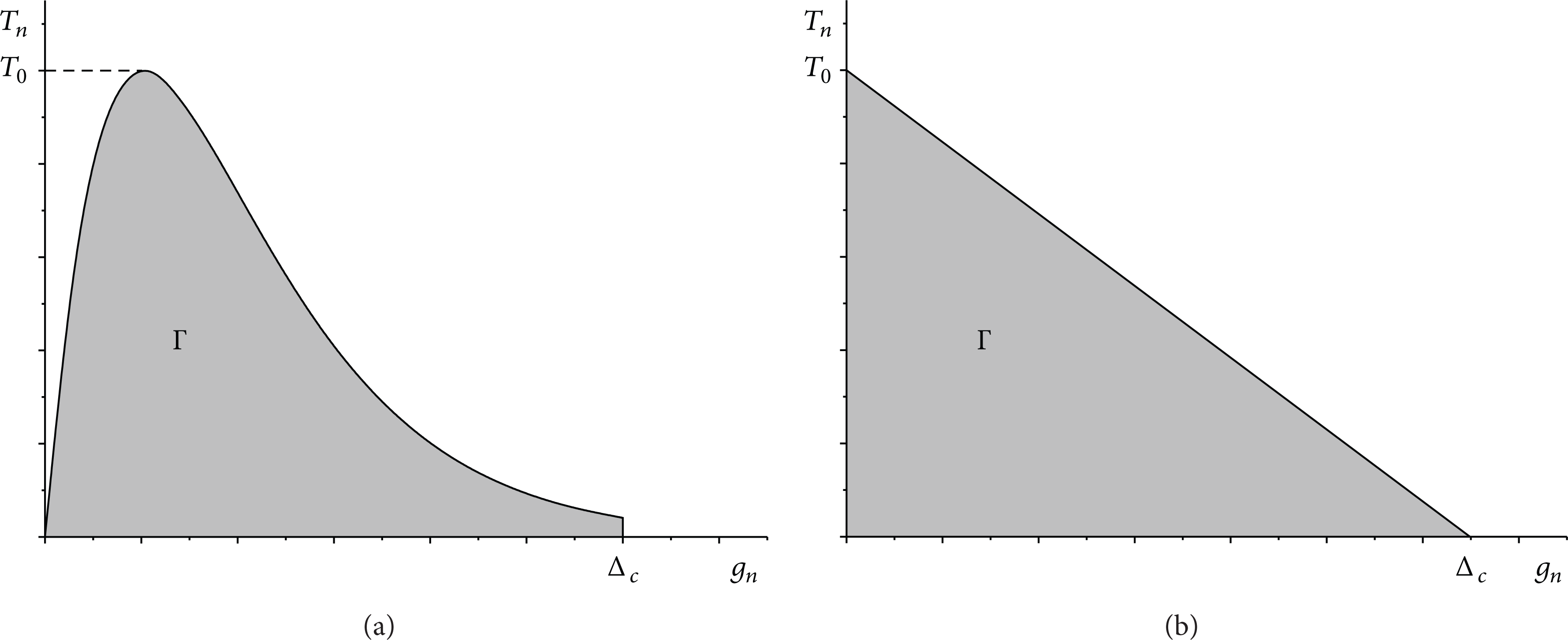
The cohesive zone model is a phenomenological model and there is no direct evidence for the formulation of traction separation law in the model. Various forms have been proposed since its initiation, as shown in Figure 2 [15]. A challenge of using cohesive zone model is to choose a proper traction separation law for different materials. As mentioned above, there are various forms for different materials They can be classified into two categories based on the model features, for example, zero traction and nonzero traction at the initial zero separation. The typical cohesive zone models of these two categories are Needleman's and Hillerborg's models as shown in Figure 3. For ductile materials, the exponential form proposed by Needleman [10] is one of the most popular traction separation laws. In this model, the traction first increases drastically to a peak value T₀, called the cohesive stress, and then decreases to zero at a critical separation Δ_c. For brittle materials, a linear decreasing form suggested by Hillerborg et al. [8] is used widely. The model starts with an infinite stiffness until the cohesive stress T₀ is reached. The area under the traction-separation curve is called the cohesive energy Γ. Recent atomistic simulations show that even for ductile materials [16], the cohesive zone model should have a nonzero critical traction. The separation cannot occur when the traction is below this critical traction. Jin and Sun [17] also conclude that the cohesive zone model must have a nonzero traction at the initial zero separation, and the cohesive traction should first increase quickly to the cohesive stress and finally decreases with further increasing separation. Based on this knowledge, we propose a new cohesive zone model, in which a parameter representing the ductility of the material is included to determine the critical traction. The proposed model is focused on the mode I crack problem.

Figure 2:

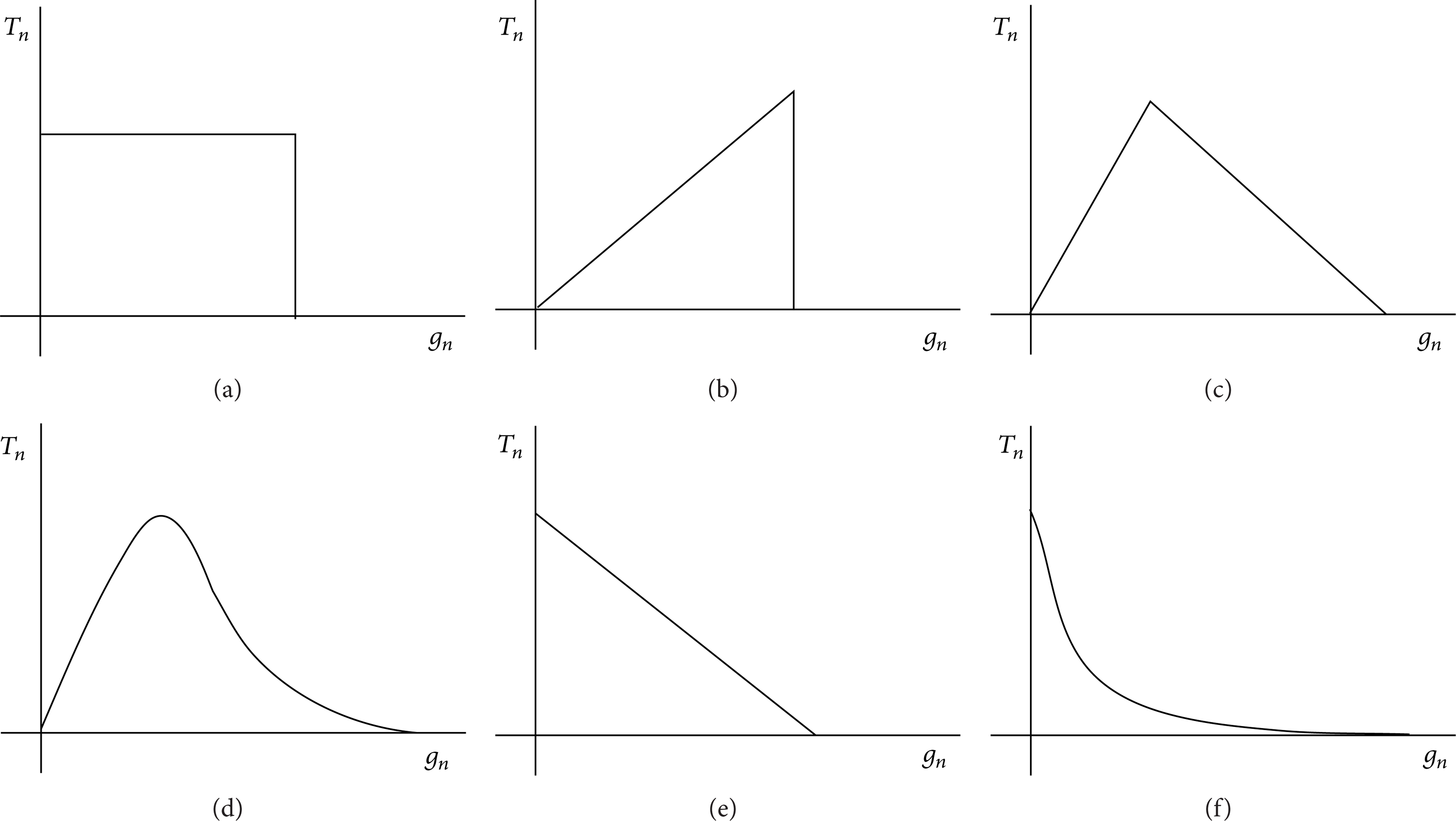
Various traction separation laws for mode I crack [15]: (a) rigid plastic law, (b) linear elastic brittle law, (c) triangular law with initial linear elastic regime followed by a linear softening regime, (d) an arbitrary traction law, often approximated with a cubic function, (e) linear softening law, (f) nonlinear softening law.

Figure 3:

Typical cohesive zone models for ductile materials (a) and brittle materials (b), recommended by Needleman [10] and Hillerborg [8], respectively.

For mode I fracture, the constitutive behavior of the cohesive zone is derived through a potential function Φ in the form

T_{n} = \frac{d Φ}{d g_{n}},

(1)

where T_n is the normal traction and g_n is the normal separation. The equation for the potential function Φ is proposed to be the form

Φ (g_{n}) = \frac{27}{16} T_{0} Δ_{0} A,

(2)

with

A = 3 {(\frac{λ Δ_{0} + g_{n}}{3 Δ_{0}})}^{4} - 8 {(\frac{λ Δ_{0} + g_{n}}{3 Δ_{0}})}^{3} + 6 {(\frac{λ Δ_{0} + g_{n}}{3 Δ_{0}})}^{2},

(3)

where Δ₀ is the cohesive length, which is the normal separation between the crack surfaces corresponding to the cohesive stress T₀ for mode I crack problem. λ is a model parameter. The relation between the traction and separation is obtained by the substitution of (2) into (1):

T_{n} = \frac{9}{4} T_{0} \frac{λ Δ_{0} + g_{n}}{Δ_{0}} {(1 - \frac{λ Δ_{0} + g_{n}}{3 Δ_{0}})}^{2} .

(4)

The parameter λ can be defined to be the ratio of yield stress to tensile strength of the material. When the value of λ ranges between 0 and 1, the model is applicable to the materials with different ductilities. Figure 4 displays the cohesive zone model with different values of the parameter λ but the same cohesive stress and cohesive energy. By setting λ = 0, the cohesive zone model returns to with Needleman's cubic traction separation form model.

Figure 4:

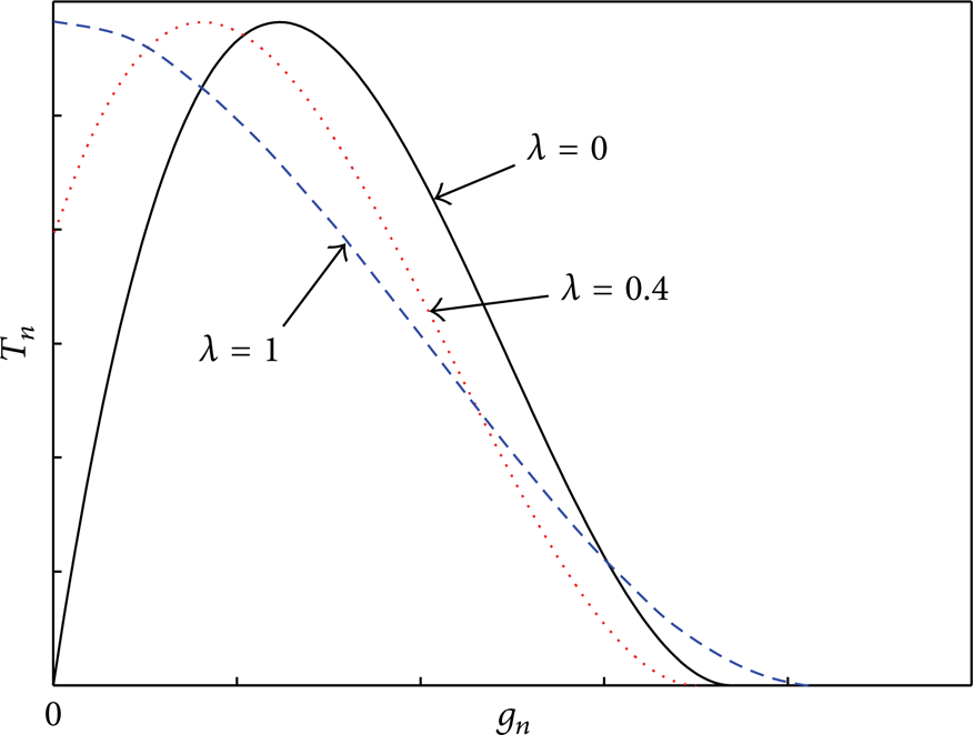
The cohesive zone models with different parameter λ but the same cohesive stress and cohesive energy Γ.

Until now, there is no unified method to determine the cohesive stress according to the author's knowledge. However, it is commonly considered to be dependent on the material property, that is, brittle or ductile. In this paper, the determination of the cohesive stress is based on the global measurement results for brittle material [18 –20] and the micromechanical study of void growth for ductile material [21 –26]. For brittle material, it fails without obvious plastic deformations, and the failure is dominated by the maximum principal stress. The material behaves linearly elastic before the maximum principal stress reaches the tensile stress. Once the tensile stress is exceeded, the material begins to fail. Based on this knowledge, the cohesive stress for the brittle materials can be taken as tensile strength of the material. For ductile material, both numerical and experimental results show that the cohesive stress strongly depends on the condition of mechanical constraint present at the crack tip [21]. The constraint state can be represented by the stress triaxiality, that is, the ratio of hydrostatic stress to equivalent stress χ = σ_h/σ_e [23]. The relationship between cohesive stress and the stress triaxiality can be determined by studying the material failure uncoupled from the crack tip problems using the so-called unit cell method [22]. In the unit cell method, the material is regarded as a periodic array of identical cells, and a representative unit cell of material under consideration is picked out to be investigated. The method is initially used to determine the constitutive relation of composite materials at the microscale [27] and recently used by researchers to determine the triaxiality dependent cohesive stress for cohesive zone model [28, 29]. To determine the relationship between cohesive stress and stress triaxiality, a representative unit cell in front of the crack tip can be studied separately from the macroscopic specimen. The constitutive equation of the material for volume element is based on the Gurson-Tvergaard-Needleman (GTN) model [24 –26], which describes the void growth and nucleation process in ductile materials. Using the unit cell method, the maximum load carrying capacity can be captured during the void growth under the given stress triaxiality, and the value of the maximum load carrying capacity is equal to the cohesive stress.

The cohesive energy Γ for both ductile and brittle materials is identical to the fracture energy, that is, the energy needed to create unit area of new crack surface. It can be experimentally measured. Once the parameters, that is, ductility λ, cohesive stress T₀, and cohesive energy Γ, are settled, the cohesive length Δ₀ is subsequently determined.

3. Numerical Implementation

The cohesive zone model is usually implemented into finite element analysis through a zero-thickness interface element, that is, cohesive element. The formulation of cohesive element is described in the following. The cohesive element is made up of two surfaces: the upper and the lower. In undeformed condition, the two surfaces of the cohesive element lie together. Under external load, the two surfaces separate but are connected by cohesive traction. The traction is calculated at the integration points according to the traction separation law. When the separation reaches a critical separation, the element fails at this point, and the contribution of the integration point to the stiffness vanishes. In the study, the bulk material is modeled by 4-node quadrilateral elements. Based on the compatibility requirements in the finite element formulation, the corresponding cohesive element is a 4-node interface element with two nodes at each surface. The cohesive element condition and its integration point position are illustrated in Figure 5. When the separation across the crack reaches a critical separation Δ_c, the solid elements connected by this cohesive element are disconnected, which implies that a real crack propagates to this element.

Figure 5:

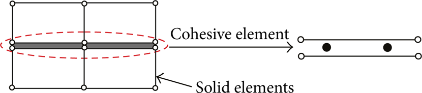
Cohesive element in two-dimension condition. The circles represent the element nodes, and the solid circles represent the Gauss points.

The stiffness matrix of the cohesive element and finite element equations can be derived from the principle of virtual work. The principle of virtual work reads

δ Π_{i} = δ Π_{e};

(5)

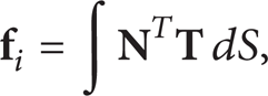
that is, the internal virtual work δΠ_i is equal to the external virtual work δΠ_e. The symbol δ denotes the variation of a quantity. The internal virtual work for the cohesive element is defined by

δ Π_{i} = \int ‍ T δ g d S,

(6)

where T is the vector of the cohesive traction, g is the separation of crack, and g = u⁺ – u⁻. Here, u⁺ and u⁻ represent the displacements of the two cohesive surfaces. S is the cohesive zone area. In finite element method, the displacement u is interpolated within the element using the nodal shape functions N and the nodal displacement q:

u = N q .

(7)

Inserting (7) into (6) leads to

δ Π_{i} = δ q^{T} f_{i},

(8)

with

f_{i} = \int N^{T} T d S,

(9)

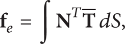
where superscript ()^T denotes a transpose operation. f_i is the equivalent internal nodal force.

The external virtual work δΠ_e is defined by

δ Π_{e} = \int \overset{—}{T} δ u d S,

(10)

where $\overset{—}{T}$ is the external traction force. Substituting (7) into (10), the external virtual work can be written as

δ Π_{e} = δ q^{T} f_{e},

(11)

with

f_{e} = \int N^{T} \overset{—}{T} d S,

(12)

where f_e is the external force.

Combining (5), (8), (9), and (11) gives

\int N^{T} T d S = f_{e} .

(13)

Since the cohesive traction is nonlinear functions of the separation, the incremental procedure is needed. The traction rate can be expressed in terms of nodal displacement velocities as

\dot{T} = \frac{\partial T}{\partial g} \dot{g} = C \dot{g} = C N \dot{q},

(14)

where C is the cohesive stiffness matrix. For two-dimensional problem, C can be expressed as

C = [\begin{bmatrix} \underset{}{\frac{\partial T_{n}}{\partial g_{n}}} & \frac{\partial T_{n}}{\partial g_{t}} \\ \frac{\partial T_{t}}{\partial g_{n}} & \frac{\partial T_{t}}{\partial g_{t}} \end{bmatrix}],

(15)

where g_t and T_t are the tangential separation and tangential traction, respectively. There are two degrees of freedom for two-dimensional problem, that is, normal and shear degrees. However, for mode I crack, all components related to shear degree are zero. Therefore, the cohesive stiffness C for mode I crack can be given as

C = [\begin{bmatrix} \underset{}{\frac{\partial T_{n}}{\partial g_{n}}} & 0 \\ 0 & 0 \end{bmatrix}] .

(16)

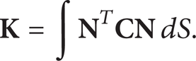
Substitution of (14) into (13) leads to the tangent stiffness matrix K in terms of incremental nodal displacements dq,

K d q = f_{e} - f_{i},

(17)

with

K = \int N^{T} C N d S .

(18)

4. Numerical Examples

In this section, four numerical examples of crack growth are carried out for two brittle materials and two ductile materials to verify the applicability and accuracy of the proposed cohesive zone model. Two brittle materials are two kinds of concrete and two ductile materials are steel 20 MnMoNi 55 and aluminium alloy AL5083. Cohesive zone model defined in (4) is implemented as the cohesive element through the user-defined subroutine UEL in the commercial finite element code ABAQUS.

4.1. Crack Growth in Brittle Materials

Two kinds of concrete, named as concrete 1 and concrete 2, are taken as examples of the brittle materials. Crack growth in three-point bending test is simulated. Experimental results taken from Fathy's work [30] are used for comparison with simulating results. The geometry, loading, and boundary conditions of three-point bending specimen are shown in Figure 6. The geometric parameters are S = 300 mm, L = 500 mm, H = 100 mm, a₀ = 33 mm, and thickness B = 100 mm. The finite element meshes for the specimen are given in Figure 7, including 1368 elements and 1451 nodes. To improve the computational efficiency, only the potential damage zone along the expected crack path is covered by the cohesive elements, and the rest of the region is occupied by 4-node linear elements.

Figure 6:

Geometry, loading, and boundary conditions of three-point bending.

Figure 7:

Finite element meshes of the three-point bending specimen.

4.1.1. Crack Growth in Concrete 1

The material properties of concrete 1 are Young's modulus E = 47.7 GPa, Poisson's ratio ν = 0.2, tensile strength σ_b = 6.18 MPa, and the cohesive energy Γ = 0.126 N/mm [30]. The parameter λ = 1 is employed. Cohesive stress T₀ = 6.18 MPa which is equal to the tensile strength. The plane strain condition is assumed.

The experimental and simulating results of force-crack mouth opening displacement (F-CMOD) curves are summarized in Figure 8 (a). It can be seen that the numerical results based on the proposed model have a good agreement with the experimental data. Moreover, the prediction of Fathy et al. [30] is also displayed in Figure 8 (a). It can be found that the simulating results are very close to Fathy's results. Figure 8 (b) shows the proposed model and Fathy's model. It is obvious that the cohesive stress in Fathy's model is higher than the proposed model which causes the slight difference of the predictions in Figure 8 (a).

Figure 8:

The simulating F-CMOD curve in comparison with the experimental as well as Fathy's results for concrete 1 [30] (a), and the comparison between proposed model and Fathy's model (b).

4.1.2. Crack Growth in Concrete 2

To further study the feasibility of the proposed model in brittle materials, another simulation has been done for concrete 2. The material properties of concrete 2 are Young's modulus E = 45.1 GPa, Poisson's ratio ν = 0.2, tensile strength σ_b = 5.82 MPa, and the cohesive energy Γ = 0.121 N/mm [30]. Parameter λ = 1 and cohesive stress T₀ = 5.82 MPa which is equal to the tensile strength. The same plane strain condition is adopted as concrete 1.

Both simulating and experimental F-CMOD curves are shown in Figure 9 (a), together with the prediction of Fathy et al. [30]. It can be found that the simulating results fit the experimental results very well in the initial part as well as the peak load value. For the postpeak response, Fathy's model gives a better result than the proposed model. Figure 9 (b) displays the comparison of the two models. It is clear to see that softening curve in Fathy's model decreases much steeper than the proposed model which could lead to the deviation of the simulating results in the postpeak response in Figure 9 (a).

Figure 9:

The simulating F-CMOD curve in comparison with the experimental as well as Fathy's results for concrete 2 [30] (a), and the comparison between proposed model and Fathy's model (b).

4.2. Crack Growth in Ductile Materials

In order to study the feasibility of the proposed model in ductile materials, two different ductile materials, that is, steel 20 MnMoNi 55 and aluminium alloy AL5083, have been employed. Crack growth tests for both materials are carried out in standard compact tension (CT) specimen which is displaced in Figure 10. Figure 11 shows the finite element meshes used in the calculation, with 3877 elements and 3996 nodes. Same as the mesh arrangement of the three-point bending specimen in Section 4.1, the potential damage zone along the expected crack path is covered by the cohesive elements, and the rest of the region is occupied by 4-node linear elements. The experimental results are documented in [31] for 20 MnMoNi 55 and [32] for AL5083.

Figure 10:

Geometry of standard CT specimen. V is the location of displacement measurement in the test, B is the thickness, and B_net is the thickness of the net section.

Figure 11:

Finite element meshes of the CT specimen.

4.2.1. Crack Growth in Steel 20 MnMoNi 55

The geometric parameters of the CT specimen for steel 20 MnMoNi 55 are W = 100 mm, a₀ = 60 mm, B = 10 mm, and B_net = 8 mm. The material properties are Young's modulus E = 210 GPa, Poisson's ratio ν = 0.3, yield stress σ_y = 465 MPa, tensile strength σ_b = 600 MPa, and the cohesive energy Γ = 120 N/mm [31]. The parameter λ calculated from the ratio of yield stress to tensile strength is 0.78. The plane strain condition is assumed in the simulation.

As mentioned above, the cohesive stress can be determined by studying the damage process at the microscale using the so-called unit cell method. At a certain point of the structure, the stress triaxiality is varied with the increase of external loading. For cohesive zone model, it results in a change of cohesive stress which depends on the stress triaxiality. The change of cohesive stress will not only make the simulation complicated but also lead to a convergency problem [29]. In this study, the maximum value of the stress triaxiality at the initial crack tip is used for evaluating the cohesive stress in unit cell method. The same treatment has been successfully used by other researchers [28, 33]. To determine the triaxiality dependent cohesive stress, the stress triaxiality at the initial point is studied first using the finite element method, in which no crack propagation is considered. The response of the stress triaxiality as the loading increases is shown in Figure 12 (a) and the parameter ρ represents the load fraction. The maximum value of stress triaxiality which represents the maximum constraint state that can endure during the whole plastic deformations is then used in the unit cell method. Once the stress triaxiality is settled, the unit cell method is used to determine the cohesive stress. Following the configuration in [29], a two-dimensional axisymmetric element is used in the unit cell method. For the material considered here, the GTN model parameters are taken from Pirondi's work [34]. Loading under various constant applied stress ratio, β = σ₁/σ₂, is considered. σ₁ is applied in the horizontal direction while σ₂ is applied in the vertical direction. The triaxiality of the element can be calculated as

χ = \frac{2 β + 1}{3 (1 - β)} .

(19)

For a given β, the applied stress and the vertical displacement at the top of the element can be evaluated. Since the maximum value of σ₂ is taken as the cohesive stress, the relationship between the cohesive stress and the stress triaxiality can be obtained. Then the maximum value of the stress triaxiality at the initial crack tip can be used to determine the cohesive stress. The relationship of the applied stress and the displacement in the vertical direction is shown in Figure 12 (b), where u is the displacement in the vertical direction and D is the length scale associated with void growth in the unit cell method. As explained in Section 2, the value of the maximum load carrying capacity is the cohesive stress, namely; T₀ = 3.44, σ_y = 1600 MPa.

Figure 12:

Determination of the cohesive stress for 20 MnMoNi 55. (a) the response of stress triaxiality as loading increases. (b) The relationship of the applied stress and the displacement in the vertical direction determined by unit cell method at χ = 2.2.

Once the cohesive parameters are determined, the crack propagation simulation is carried out. The simulating as well as the experimental force-displacement (F-V) curves are displayed in Figure 13 (a). The numerical prediction obtained by Cornec et al. [31] is also displayed. For whole force-displacement curve, the proposed model and Cornec's model [31] almost give the same values and match the experimental results accurately. Figure 13 (b) shows the proposed model and Cornec's model. The difference between the two models is obvious. It seems that for the ductile materials, the simulating results are not sensitive to the form of the cohesive zone model.

Figure 13:

Comparison of experimental [31] and predicted F-V curves for steel 20 MnMoNi 55 (a), and comparison of proposed model and Cornec's model (b).

4.2.2. Crack Propagation in Aluminium Alloy AL5083

The CT specimen used for aluminium alloy AL5083 has different geometric parameters from that for steel 20 MnMoNi 55, which are W = 50 mm, a₀ = 25 mm, and B = B_net = 3 mm. The material properties of AL5083 are Young's modulus E = 68 GPa, Poisson's ratio ν = 0.33, yield stress σ_y = 243 MPa, tensile strength σ_b = 350 MPa, and the cohesive energy Γ = 10 N/mm [32]. In the simulation, plane stress condition is adopted. Parameter λ = 0.69 which is calculated by the ratio of yield stress to tensile strength. Using the same method mentioned in Section 4.2.1, the stress triaxiality is calculated and depicted in Figure 14 (a). The maximum value of stress triaxiality is 0.63, which will be used in the unit cell method. The GTN model parameters in the unit cell method for this material are determined by Gao et al. [35]. The relationship of the applied stress and the displacement in the vertical direction is determined by unit cell approach and shown in Figure 14 (b). From Figure 14 (b), the cohesive stress is determined as T₀ = 2.3, σ_y = 560 MPa.

Figure 14:

Determination of the cohesive stress for AL5083. (a) The response of stress triaxiality with the increase of load fraction. (b) The relationship of the applied stress and the displacement in the vertical direction determined by unit cell method at χ = 0.63.

The comparison between the simulating and experimental results, as well as the prediction by Scheider et al. [32], is shown in Figure 15 (a). The comparison between proposed model and Scheider's model is given in Figure 15 (b). For whole force-displacement (F-V) curve, the proposed model presents a better agreement with the experimental results than Scheider's model. Same as in the case of steel 20 MnMoNi 55, the proposed model shows a big difference with Scheider's model, as shown in Figure 15 (b).

Figure 15:

Comparison of experimental [32] and predicted F-V curves for AL5083 (a) and comparison of proposed model and Scheider's model (b).

5. Conclusions

In the present work, a unified cohesive zone model has been proposed, which is applicable for both brittle and ductile materials. To verify the feasibility of the proposed model, several numerical examples have been carried out, and the following conclusions are obtained.

Introducing a new parameter into conventional cohesive zone model to characterize the ductility of the material can lead to a unified cohesive zone model which is suitable for both brittle and ductile materials.

In the present investigation, all the parameters in cohesive zone model are calibrated independent on the cohesive zone model, that is, no fitting experimental data is needed, and this leads to a high predictive ability of the model.

The simulating results have a good agreement with the experimental data, which proves the applicability and accuracy of the proposed model. Moreover, the form of the cohesive zone model is not crucial for ductile materials because the different cohesive zone models can predict nearly same crack growth behavior for ductile materials.

Footnotes

Nomenclature

Acknowledgment

This study is based upon the work supported by the National Natural Science Foundation of China (Grant no. 51005020).

References

Dugdale

D. S.

, “Yielding of steel sheets containing slits,” Journal of the Mechanics and Physics of Solids, vol. 8, no. 2, pp. 100–104, 1960.

Barenblatt

G. I.

, “The mathematical theory of equilibrium cracks in brittle fracture,” Advances in Applied Mechanics, vol. 7, pp. 55–129, 1962.

van den Bosch

M. J.

Schreurs

P. J. G.

, and Geers

M. G. D.

, “An improved description of the exponential Xu and Needleman cohesive zone law for mixed-mode decohesion,” Engineering Fracture Mechanics, vol. 73, no. 9, pp. 1220–1234, 2006.

Liu

Xiang

, and Yuan

, “Prediction of 3D small fatigue crack propagation in shot-peened specimens,” Computational Materials Science, vol. 46, no. 3, pp. 566–571, 2009.

Liu

Yuan

, and Liao

, “Prediction of fatigue crack growth and residual stress relaxations in shot-peened material,” Materials Science and Engineering A, vol. 527, no. 21–22, pp. 5962–5968, 2010.

X.-P.

Needleman

, and Abraham

F. F.

, “Effect of inhomogeneities on dynamic crack growth in an elastic solid,” Modelling and Simulation in Materials Science and Engineering, vol. 5, no. 5, pp. 489–516, 1997.

Miller

Freund

L. B.

, and Needleman

, “Energy dissipation in dynamic fracture of brittle materials,” Modelling and Simulation in Materials Science and Engineering, vol. 7, no. 4, pp. 573–586, 1999.

Hillerborg

Modéer

, and Petersson

P.-E.

, “Analysis of crack formation and crack growth in concrete by means of fracture mechanics and finite elements,” Cement and Concrete Research, vol. 6, no. 6, pp. 773–781, 1976.

Needleman

, “A continuum model for void nucleation by inclusion debonding,” Journal of Applied Mechanics, Transactions ASME, vol. 54, no. 3, pp. 525–531, 1987.

10.

Needleman

, “An analysis of decohesion along an imperfect interface,” International Journal of Fracture, vol. 42, no. 1, pp. 21–40, 1990.

11.

Yuan

Lin

, and Cornec

, “Verification of a cohesive zone model for ductile fracture,” Journal of Engineering Materials and Technology, Transactions of the ASME, vol. 118, no. 2, pp. 192–200, 1996.

12.

Geubelle

P. H.

and Baylor

J. S.

, “Impact-induced delamination of composites: a 2D simulation,” Composites Part B: Engineering, vol. 29, no. 5, pp. 589–602, 1998.

13.

Tvergaard

and Hutchinson

J. W.

, “The relation between crack growth resistance and fracture process parameters in elastic-plastic solids,” Journal of the Mechanics and Physics of Solids, vol. 40, no. 6, pp. 1377–1397, 1992.

14.

Chaboche

J. L.

Girard

, and Levasseur

, “On the interface debonding models,” International Journal of Damage Mechanics, vol. 6, no. 3, pp. 220–257, 1997.

15.

Nairn

J. A.

, “Analytical and numerical modeling of R curves for cracks with bridging zones,” International Journal of Fracture, vol. 155, no. 2, pp. 167–181, 2009.

16.

Krull

and Yuan

, “Suggestions to the cohesive traction-separation law from atomistic simulations,” Engineering Fracture Mechanics, vol. 78, no. 3, pp. 525–533, 2011.

17.

Jin

Z.-H.

and Sun

C. T.

, “Cohesive fracture model based on necking,” International Journal of Fracture, vol. 134, no. 2, pp. 91–108, 2005.

18.

Wells

G. N.

and Sluys

L. J.

, “A new method for modelling cohesive cracks using finite elements,” International Journal for Numerical Methods in Engineering, vol. 50, no. 12, pp. 2667–2682, 2001.

19.

Hansbo

and Hansbo

, “A finite element method for the simulation of strong and weak discontinuities in solid mechanics,” Computer Methods in Applied Mechanics and Engineering, vol. 193, no. 33–35, pp. 3523–3540, 2004.

20.

Mergheim

Kuhl

, and Steinmann

, “A finite element method for the computational modelling of cohesive cracks,” International Journal for Numerical Methods in Engineering, vol. 63, no. 2, pp. 276–289, 2005.

21.

Brocks

Klingbeil

Künecke

, and Sun

D. Z.

, “Application of the Gurson model to ductile tearing resistance,” in Constraint Effects in Fracture: Theory and Applications, Kirk

and Bakker

, Eds., vol. 144 of ASTM STP, pp. 232–252, American Society for Testing and Materials, Philadelphia, Pa, USA, 1995.

22.

Brocks

Sun

D.-Z.

, and Hönig

, “Verification of the transferability of micromechanical parameters by cell model calculations with visco-plastic materials,” International Journal of Plasticity, vol. 11, no. 8, pp. 971–989, 1995.

23.

Siegmund

and Brocks

, “Tensile decohesion by local failure criteria,” Technische Mechanik, vol. 18, pp. 261–270, 1998.

24.

Gurson

A. L.

, “Continuum theory of ductile rupture by void nucleation and growth: part I—yield criteria and flow rules for porous ductile media,” Journal of Engineering Materials and Technology, Transactions of the ASME, vol. 99, no. 1, pp. 2–15, 1977.

25.

Tvergaard

, “On localization in ductile materials containing spherical voids,” International Journal of Fracture, vol. 18, no. 4, pp. 237–252, 1982.

26.

Needleman

and Tvergaard

, “An analysis of ductile rupture in notched bars,” Journal of the Mechanics and Physics of Solids, vol. 32, no. 6, pp. 461–490, 1984.

27.

Aboudi

, “Transient waves in composite materials,” Wave Motion, vol. 9, no. 2, pp. 141–156, 1987.

28.

Siegmund

and Brocks

, “Numerical study on the correlation between the work of separation and the dissipation rate in ductile fracture,” Engineering Fracture Mechanics, vol. 67, no. 2, pp. 139–154, 2000.

29.

Scheider

, “Derivation of separation laws for cohesive models in the course of ductile fracture,” Engineering Fracture Mechanics, vol. 76, no. 10, pp. 1450–1459, 2009.

30.

Fathy

A. M.

Sanz

Sancho

J. M.

, and Planas

, “Determination of the bilinear stress-crack opening curve for normal- and high-strength concrete,” Fatigue and Fracture of Engineering Materials and Structures, vol. 31, no. 7, pp. 539–548, 2008.

31.

Cornec

Scheider

, and Schwalbe

K.-H.

, “On the practical application of the cohesive model,” Engineering Fracture Mechanics, vol. 70, no. 14, pp. 1963–1987, 2003.

32.

Scheider

Schödel

Brocks

, and Schönfeld

, “Crack propagation analyses with CTOA and cohesive model: comparison and experimental validation,” Engineering Fracture Mechanics, vol. 73, pp. 252–263, 2006.

33.

Banerjee

and Manivasagam

, “Triaxiality dependent cohesive zone model,” Engineering Fracture Mechanics, vol. 76, no. 12, pp. 1761–1770, 2009.

34.

Pirondi

Bonora

Steglich

Brocks

, and Hellmann

, “Simulation of failure under cyclic plastic loading by damage models,” International Journal of Plasticity, vol. 22, no. 11, pp. 2146–2170, 2006.

35.

Gao

Zhang

Zhou

Graham

S. M.

Hayden

, and Roe

, “On stress-state dependent plasticity modeling: significance of the hydrostatic stress, the third invariant of stress deviator and the non-associated flow rule,” International Journal of Plasticity, vol. 27, no. 2, pp. 217–231, 2011.

Finite Element Analysis for Brittle and Ductile Fracture Using a Unified Cohesive Zone Model

Abstract

1. Introduction

2. Cohesive Zone Model

3. Numerical Implementation

4. Numerical Examples

4.1. Crack Growth in Brittle Materials

4.1.1. Crack Growth in Concrete 1

4.1.2. Crack Growth in Concrete 2

4.2. Crack Growth in Ductile Materials

4.2.1. Crack Growth in Steel 20 MnMoNi 55

4.2.2. Crack Propagation in Aluminium Alloy AL5083

5. Conclusions

Footnotes

Nomenclature

Acknowledgment

References