On Adaptive Energy-Efficient Transmission in WSNs

Abstract

One of the major challenges in design of wireless sensor networks (WSNs) is to reduce energy consumption of sensor nodes to prolong lifetime of finite capacity batteries. In this paper, we propose energy-efficient adaptive scheme for transmission (EAST) in WSNs. EAST is an IEEE 802.15.4 standard compliant. In this scheme, open-looping feedback process is used for temperature-aware link quality estimation and compensation, wherea closed-loop feedback process helps to divide network into three logical regions to minimize overhead of control packets. Threshold on transmitter power loss ( ${\text{RSSI}}_{\text{loss}}$ ) and current number of nodes ( $n_c$ (t)) in each region help to adapt transmit power level ( $P_{\text{level}}$ ) according to link quality changes due to temperature variation. Evaluation of the proposed scheme is done by considering mobile sensor nodes and reference node both static and mobile. Simulation results show that the proposed scheme effectively adapts transmission $P_{\text{level}}$ to changing link quality with less control packets overhead and energy consumption as compared to classical approach with single region in which maximum transmitter $P_{\text{level}}$ assigned to compensate temperature variation.

1. Introduction

WSNs are currently being considered for many applications, including industrial, security surveillance, medical, environmental, and weather monitoring. Due to limited battery lifetime at each sensor node, minimizing transmitter $P_{\text{level}}$ to increase energy efficiency and network lifetime is useful. Sensor nodes consist of three parts: sensing unit, processing unit, and transceiver [1]. Limited battery requires low power sensing, processing, and communication system. Energy efficiency is of paramount interest, and optimal WSN should consume minimum amount of power.

In WSNs, sensor nodes are widely deployed in different environments to collect data. As sensor nodes usually operate on limited battery, each sensor node communicates using a low power wireless link, and link quality varies significantly due to environmental dynamics like temperature and humidity. Therefore, while maintaining good link quality between sensor nodes, we need to reduce energy consumption for data transmission to extend network lifetime [2–4]. IEEE802.15.4 is a standard used for low energy, low data rate applications like WSN. This standard operates at frequency of 2.45 GHz with channels up to 16 and data rate of 250 kbps.

To efficiently compensate link quality changes due to temperature variations, we propose a new scheme for $P_{\text{level}}$ control EAST that improves network lifetime while achieving required reliability between sensor nodes. This scheme is based on combination of open-loop and closed-loop feedback processes in which we divide network into three regions on basis of threshold on RSSI_loss for each region. In open-loop process, each node estimates link quality using its temperature sensor. Estimated link quality degradation is then effectively compensated using closed-loop feedback process by applying the proposed scheme. In closed-loop feedback process, appropriate transmission $P_{\text{level}}$ control is obtained which assigns substantially less power than that required in existing transmission power control schemes.

The rest of the paper is organized as follows. Section 2 briefs the related existing work and motivation for this work. In Section 3, we provide the readers with our proposed scheme. In Section 4, we model our proposed scheme. Experimental results have been given in Section 5.

2. Related Work and Motivation

To transmit data efficiently over wireless channels in WSNs, existing schemes set some minimum transmission $P_{\text{level}}$ for maintaining reliability. These schemes either decrease interference among sensor nodes or increase unnecessary energy consumption. In order to adjust transmission $P_{\text{level}}$ , a reference node periodically broadcasts a beacon message. When nodes hear a beacon message from a reference node, nodes transmit an ACK message. Through this interaction, the reference node estimates connectivity between nodes.

In local mean algorithm (LMA), a reference node broadcasts LifeMsg message. Nodes transmit LifeAckMsg after they receive LifeMsg. Reference nodes count the number of LifeAckMsgs and transmission $P_{\text{level}}$ to maintain appropriate connectivity. For example, if the number of LifeAckMsgs is less than NodeMinThresh, transmission $P_{\text{level}}$ is increased. In contrast, if the number of LifeAckMsgs is more than NodeMaxThreshold transmission, $P_{\text{level}}$ is decreased. As a result, they provide improvement of network lifetime in a sufficiently connected network. However, LMA only guarantees connectivity between nodes and cannot estimate link quality [5].

Local Information No Topology/Local Information Link-state Topology (LINT/LILT), and Dynamic Transmission Power Control (DTPC) use RSSI_loss to estimate transmitter $P_{\text{level}}$ . Nodes exceeding threshold RSSI_loss are regarded as neighbor nodes with reliable links. Transmission $P_{\text{level}}$ is also controlled by packet reception ratio (PRR) metric. As for the neighbor selection method, three different methods have been used in the literature: connectivity based, PRR based, and RSSI_loss based. In LINT/LILT, a node maintains a list of neighbors whose RSSI_loss values are higher than the threshold RSSI_loss, and it adjusts the radio transmission $P_{\text{level}}$ if the number of neighbors is outside the predetermined bound. In LMA/LMN, a node determines its range by counting how many other nodes acknowledged to the beacon message it has sent [6].

Adaptive transmission power control (ATPC) adjusts transmission $P_{\text{level}}$ dynamically according to spatial and temporal effects. This scheme tries to adapt link quality that changes over time by using closed-loop feedback. However, in large-scale WSNs, it is difficult to support scalability due to serious overhead required to adjust transmission $P_{\text{level}}$ of each link. The result of applying ATPC is that every node knows the proper transmission $P_{\text{level}}$ to use for each of its neighbors, and every node maintains good link qualities with its neighbors by dynamically adjusting the transmission $P_{\text{level}}$ through on-demand feedback packets. Uniquely, ATPC adopts a feedback-based and pairwise transmission $P_{\text{level}}$ control. By collecting the link quality history, ATPC builds a model for each neighbor of the node. This model represents an in situ correlation between transmission $P_{\text{level}}$ and link qualities. With such a model, ATPC tunes the transmission $P_{\text{level}}$ according to monitored link quality changes. The changes of transmission $P_{\text{level}}$ reflect changes in the surrounding environment [7].

Existing approaches estimate variety of link quality indicators by periodically broadcasting a beacon message. In addition, feedback process is repeated for adaptively controlling transmission $P_{\text{level}}$ . In adapting link quality for environmental changes, where temperature variation occurs, packet overhead for transmission $P_{\text{level}}$ control should be minimized. Reducing the number of control packets while maintaining reliability is an important technical issue [8].

Radio communication quality between low power sensor devices is affected by spatial and temporal factors. The spatial factors include the surrounding environment, such as terrain and the distance between the transmitter and the receiver. Temporal factors include surrounding environmental changes in general, such as weather conditions (temperature). To establish an effective transmission $P_{\text{level}}$ control mechanism, we need to understand the dynamics between link quality and RSSI_loss values. Wireless link quality refers to the radio channel communication performance between a pair of nodes. PRR is the most direct metric for link quality. However, the PRR value can only be obtained statistically over a long period of time. RSSI_loss can be used effectively as binary link quality metrics for transmission $P_{\text{level}}$ control [9].

Radio irregularity results in radio signal strength variation in different directions, but the signal strength at any point within the radio transmission range has a detectable correlation with transmission power in a short time period. There are three main reasons for the fluctuation in the RSSI_loss. First, fading causes signal strength variation at any specific distance. Second, the background noise impairs the channel quality seriously when the radio signal is not significantly stronger than the noise signal. Third, the radio hardware does not provide strictly stable functionality [10].

Since the variation is small, this relation can be approximated by a linear curve. The correlation between RSSI_loss and transmission $P_{\text{level}}$ is approximately linear. Correlation between transmission $P_{\text{level}}$ and RSSI_loss is largely influenced by environments, and this correlation changes over time. Both the shape and the degree of variation depend on the environment. This correlation also dynamically fluctuates when the surrounding environmental conditions change. The fluctuation is continuous, and the changing speed depends on many factors, among which the degree of environmental variation is one of the main factors [11].

Proposing energy-efficient transmission scheme EAST helps efficiently compensate link quality changes due to temperature variation. Estimated packet overhead for adaptive power control temperature measured by sensors is utilized to adjust transmission $P_{\text{level}}$ for all three regions based on RSSI_loss. Compared to single region in which large overhead of control packets occurs even due to small change in link quality, multiple regions have reduced overhead. Closed-loop feedback process is executed to minimize control packets overhead and required transmitter $P_{\text{level}}$ .

3. Proposed Energy-Efficient Transmission Scheme

In this section, we present-energy efficient transmission scheme that maintains link quality during temperature variation in wireless environment. It utilizes open-loop process based on sensed temperature information according to temperature variation. Closed-loop feedback process based on control packets is further used to accurately adjust transmission $P_{\text{level}}$ . By adopting both open-loop and closed-loop feedback processes, we divide network into three regions: A, B, and C for high, medium, and low RSSI_loss, respectively.

In order to assign minimum and reachable transmission $P_{\text{level}}$ to each link, EAST is designed. EAST has two phases, that is, initial and run-time. In initial phase, reference node builds a model for nodes in network. In run time phase based on previous model, EAST adapts the link quality to dynamically maintain each link with respect to time. In a relatively stable network, control overhead occurs only in measuring link quality in initial phase. But in a relatively unstable network because link quality is continuously changing, initial phase is repeated and serious overhead occurs. Before we present block diagram for the proposed scheme, some variables are defined as follows: (1) current nodes in a region $n_c(t)$ , (2) desired nodes in a region $n_d(t)$ , and (3) error: $e(t)=n_d(t)-n_c(t)$ , (4) $P_{\text{level}}$ .

Figure 1 shows system block diagram of the proposed scheme. PRR, ACK, and RSSI_loss are used to determine connectivity. ACK estimates connectivity, but it cannot determine link quality. PRR estimates connectivity accurately, but it causes significant overhead [8]. In our scheme, we use RSSI_loss for connectivity estimation, which measures connectivity with relatively low overhead.

Figure 1

Block diagram.

Power controller adjusts transmission $P_{\text{level}}$ by utilizing both the number of current nodes and the temperature sensed at each node. Since power controller is operated not merely by comparing number of current nodes with desired nodes but by using temperature-compensated $P_{\text{level}}$ , it can reach the desired $P_{\text{level}}$ rapidly. If temperature is changing then temperature compensation is executed on basis of relationship between temperature and RSSI_loss. Network connectivity is maintained with low overhead by reducing feedback process between nodes which is achieved due to logical division of network.

Transmission power loss due to temperature variation was formulated using the relationship between RSSI_loss and temperature experimented by Bannister et al. The mathematical expression for RSSI_loss due to temperature variation is as follows [12]:

$$\begin{array}{cc}& {\text{RSSI}}_{\text{loss}}\left[\text{dBm}\right]=\mathrm{0.1996}*\left(T\left[{}^{°}\text{C}\right]-25\left[{}^{°}\text{C}\right]\right).\end{array}$$

(1)

To compensate RSSI_loss estimated from (1), we have to control output $P_{\text{level}}$ of radio transmitter accordingly. The relationship between required transmitter $P_{\text{level}}$ and RSSI_loss is formulated using least square approximation [12] as follows:

$$\begin{array}{cc}& P_{\text{level}}={\left[\frac{\left({\text{RSSI}}_{\text{loss}}+40\right)}{12}\right]}^{\mathrm{2.91}}.\end{array}$$

(2)

Based on (1) and (2), we obtain appropriate $P_{\text{level}}$ to compensate RSSI_loss due to temperature variation. To compensate path loss due to distance between each sensor node in WSN, free-space model helps to estimate actual required transmitter power. After the addition of RSSI_loss due to temperature variation in (3), we estimate actual required transmitter power between each sensor node. For free-space path loss model, we need the number of nodes in a network (N), the distance between each node (d), ( $E_b/N_o$ ) depending upon ( $\text{SNR}$ ), spectral efficiency (η), frequency (f), and Receiver Noise Figure (RNF):

$$\begin{array}{l}{P}_t\left[\text{dBm}\right]\\ \hspace{1em}=\left[\eta *\left(\frac{E_b}{N_0}\right)*mkTB*{\left(\frac{4\pi d}{\lambda }\right)}^2+\text{RNF}\right]+{\text{RSSI}}_{\text{loss}}.\end{array}$$

(3)

Parameters for propose scheme are (1) threshold RSSI_loss for each region, (2) desired nodes in each region $n_d(t)=n_c(t)-5$ , and (3) transmission power level $P_{\text{level}}$ for each region (Table 1).

Table 1

Estimated parameters.

$N(\text{A},\text{B},\text{C})$	46, 30, 24
$n_d(\text{A},\text{B},\text{C})$	41, 25, 19
$n_c(\text{A},\text{B},\text{C})$	41, 22, 17
Threshold power $\text{level}\hspace{0.17em}(\text{A},\text{B},\text{C})$	43.24, 31.77, 22.21
Nodes above threshold RSSIloss $(\text{A},\text{B},\text{C})$	23, 11, 8
Nodes below threshold RSSIloss ( $\text{A},\text{B},\text{C}$ )	18, 11, 9
PRR ( $\text{A},\text{B},\text{C}$ )	(80–98), (70–96), (63–97)%
Threshold RSSIloss ( $\text{A},\text{B},\text{C}$ )	3.78, $-\mathrm{0.61}$ , $-\mathrm{5.17}$  dBm

Threshold RSSI_loss is the minimum value required to maintain link reliability. A reference node broadcasts beacon message periodically to nodes and waits for ACKs. If ACKs are received from nodes, then RSSI_loss is estimated for logical division of network, number of nodes with high RSSI_loss considered in region A, medium RSSI_loss considered in region B, and low RSSI_loss in region C. If ${\text{RSSI}}_{\text{loss}}\ge {\text{RSSI}}_{\text{loss}}$ threshold and $n_c(t)\ge n_d(t)$ , then threshold transmitter $P_{\text{level}}$ is assigned if for similar case $n_c(t)<n_d(t)$ then similar transmitter $P_{\text{level}}$ is assigned and if ${\text{RSSI}}_{\text{loss}}<{\text{RSSI}}_{\text{loss}}$ threshold then by default keep the same transmitter $P_{\text{level}}$ as shown in Algorithm 1.

Algorithm 1: EAST algorithm.

(1)   $r\leftarrow$   Number of rounds  

(2) $N\leftarrow$   Number of nodes in Network

(3) $d\leftarrow$   Distance between each node and reference node  

(4) $T\leftarrow$   Temperature for each node

(5) $RSS{I}_{loss}\leftarrow$   Transmission power loss for each node  

(6)    $P_{level}\leftarrow$   Power level for each node  

(7)    $P_t\leftarrow$   Transmitter power for each node  

(8)    $Region\hspace{0.17em}\hspace{0.17em}A\leftarrow HighRSS{I}_{loss}$   

(9)    $Region\hspace{0.17em}\hspace{0.17em}B\leftarrow MediumRSS{I}_{loss}$   

(10) $Region\hspace{0.17em}\hspace{0.17em}C\leftarrow LowRSS{I}_{loss}$   

(11)   $n_c(t)\leftarrow$   Current number of nodes  

(12) $n_d(t)\leftarrow$   Desired number of nodes  

(13) if $RSS{I}_{loss}(A,B,C)\ge RSS{I}_{loss}(Threshold)$ then

(14)  if $n_c(t)(A,B,C)\ge n_d(t)(A,B,C)$ then

(15)    $RSS{I}_{loss}(new)(A,B,C)=RSS{I}_{loss}(Threshold)$   

(16)  else

(17)    $RSS{I}_{loss}(new)(A,B,C)=RSS{I}_{loss}(A,B,C)$   

(18)  end if

(19)  end if

(20) if $RSS{I}_{loss}(A,B,C)<RSS{I}_{loss}(Threshold)$ then

(21)  $RSS{I}_{loss}(new)(A,B,C)=RSS{I}_{loss}(A,B,C)$   

(22) end if

(23)  $P_{Save}$ $(A,B,C)=P_{level}-P_{level}(new)(A,B,C)$   

Figure 2 shows complete flow chart for reference node. A node senses temperature by using locally installed sensor and checks if a temperature change is detected. If there is any temperature change, compensation process is executed on the basis of (1) and (2). Nodes send an ACK message including temperature change information with a newly calculated $P_{\text{level}}$ . Applying this temperature-aware compensation scheme, we can reduce overhead caused by conventional scheme in changing temperature environments.

Figure 2

Flow chart of reference node.

4. Mathematical Representation of the Proposed Scheme

Let suppose that we have 100 nodes in a network that are randomly deployed represented as ( $N_i$ ). Nodes are placed at different locations in a square area of 100*100 m, and distance ( $d_i$ ) between them is from 1 to 100 m. For the given environment, temperature ( $T_i$ ) can have values in the range −10°C ≤ $T_i$ ≤ 53°C for all $i\hspace{0.17em}ϵ\hspace{0.17em}N$ .

RSSI_loss due to the temperature variation can be formulated using the relation between RSSI_loss and the temperature experimented in [12]. Equation for the RSSI_loss for the temperature variation is as follows:

$$\begin{array}{cc}& \text{RSS}{\text{I}}_{\text{loss}}\left(i\right)\left[\text{dBm}\right]=\mathrm{0.1996}*\left(T_i\left[{}^{°}\text{C}\right]-25\left[{}^{°}\text{C}\right]\right).\end{array}$$

(4)

The relation between $P_{\text{level}}$ and RSSI_loss is formulated by using a least square approximation [12]:

$$\begin{array}{cc}& P_{\text{level}}\left(i\right)={\left[\frac{{\text{RSSI}}_{\text{loss}}\left(i\right)+40}{12}\right]}^{\mathrm{2.91}}.\end{array}$$

(5)

Maximum, minimum, and average value of RSSI_loss for all nodes in network can be formulated as follows:

$$\begin{array}{l}\text{RSS}{\text{I}}_{\text{loss}}\left(\min \right)=\min \left(\text{RSS}{\text{I}}_{\text{loss}}\left(i\right)\right),\\ \text{RSS}{\text{I}}_{\text{loss}}\left(\max \right)=\max \left(\text{RSS}{\text{I}}_{\text{loss}}\left(i\right)\right),\\ \text{RSS}{\text{I}}_{\text{loss}}\left(\text{avg}\right)\\ \hspace{1em}=\frac{\left(\min \left(\text{RSS}{\text{I}}_{\text{loss}}\left(i\right)\right)+\max \left(\text{RSS}{\text{I}}_{\text{loss}}\left(i\right)\right)\right)}{2}.\end{array}$$

(6)

After finding maximum and minimum values of $\text{RSS}{\text{I}}_{\text{loss}}$ , we will define upper and lower limits of $\text{RSS}{\text{I}}_{\text{loss}}$ to divide the network into three regions. A counter is also initialized at zero to count the number of nodes in each region. Then we define upper and lower bounds and check condition; nodes that follow this condition are considered to be in region A for all $i\hspace{0.17em}\hspace{0.17em}ϵ\hspace{0.17em}N$ :

$$\begin{array}{cc}& \text{RSS}{\text{I}}_{\text{loss}}\left(\text{A}\hspace{0.17em}\max \right)=\max \left(\text{RSS}{\text{I}}_{\text{loss}}\left(i\right)\right),\\ \text{RSS}{\text{I}}_{\text{loss}}(\text{A}\hspace{0.17em}\min )=\text{RSS}{\text{I}}_{\text{loss}}\left(\text{avg}\right)+2\end{array}$$

(7)

•  

  $\text{count}=0$ ;

•  

  ${\text{count}}_{\text{A}}=\text{count}+1$

•  

  Given that for all $i\hspace{0.17em}ϵ\hspace{0.17em}N$ ;

•  

  $\text{RSS}{\text{I}}_{\text{loss}}(i)\le \text{RSS}{\text{I}}_{\text{loss}}(\text{A}\hspace{0.17em}\max )$ and $\text{RSS}{\text{I}}_{\text{loss}}(i)>\text{RSS}{\text{I}}_{\text{loss}}(\text{A}\hspace{0.17em}\min )$ .

Similarly, we define upper and lower limits for regions B and C and also check nodes that follow given conditions are said to be in region, B and C, respectively:

$$\begin{array}{cc}& \text{RSS}{\text{I}}_{\text{loss}}\left(\text{B}\hspace{0.17em}\max \right)=\text{RSS}{\text{I}}_{\text{loss}}\left(\text{avg}\right)+2,\\ \text{RSS}{\text{I}}_{\text{loss}}\left(\text{B}\hspace{0.17em}\min \right)=\text{RSS}{\text{I}}_{\text{loss}}\left(\text{avg}\right)-2.\end{array}$$

(8)

•  

  $\text{count}=0$ ;

•  

  ${\text{count}}_{\text{B}}=\text{count}+1$ .

•  

  Given that for all $i\hspace{0.17em}ϵ\hspace{0.17em}N$ ,

•  

  $\text{RSS}{\text{I}}_{\text{loss}}(i)\le \text{RSS}{\text{I}}_{\text{loss}}(\text{B}\hspace{0.17em}\max )$ and $\text{RSS}{\text{I}}_{\text{loss}}(i)>\text{RSS}{\text{I}}_{\text{loss}}(\text{B}\hspace{0.17em}\min )$

  $$\begin{array}{cc}& \text{RSS}{\text{I}}_{\text{loss}}\left(\text{C}\hspace{0.17em}\min \right)=\min \left(\text{RSS}{\text{I}}_{\text{loss}}\left(i\right)\right)\\ \text{RSS}{\text{I}}_{\text{loss}}\left(\text{C}\hspace{0.17em}\max \right)=\text{RSS}{\text{I}}_{\text{loss}}\left(\text{avg}\right)-2\end{array}$$

  (9)

•  

  $\text{count}=0$ ;

•  

  ${\text{count}}_{\text{C}}=\text{count}+1$ .

•  

  Given that forall $i\hspace{0.17em}ϵ\hspace{0.17em}N$ ,

•  

  $\text{RSS}{\text{I}}_{\text{loss}}(i)\le \text{RSS}{\text{I}}_{\text{loss}}(\text{C}\hspace{0.17em}\max )$ and $\text{RSS}{\text{I}}_{\text{loss}}(i)\ge \text{RSS}{\text{I}}_{\text{loss}}(\text{C}\hspace{0.17em}\min )$ .

To apply our proposed scheme EAST, we need to define threshold on $\text{RSS}{\text{I}}_{\text{loss}}$ for each region for energy-efficient communication between sensor nodes. Threshold on $\text{RSS}{\text{I}}_{\text{loss}}$ for each region depends upon $\text{RSS}{\text{I}}_{\text{loss}}$ of all nodes in a particular region and the number of nodes in that region. Threshold on $\text{RSS}{\text{I}}_{\text{loss}}$ for each region is defined as follows:

$$\begin{array}{cc}& \text{RSS}{\text{I}}_{\text{loss}}\left({\text{Threshold}}_{\text{A}}\right)={\displaystyle \sum }_{i=1}^{{\text{count}}_{\text{A}}}‍\frac{\left(\text{RSS}{\text{I}}_{\text{loss}}\left(i\right)\right)}{{\text{count}}_{\text{A}}},\\ \text{RSS}{\text{I}}_{\text{loss}}\left({\text{Threshold}}_{\text{B}}\right)={\displaystyle \sum }_{i=1}^{{\text{count}}_{\text{B}}}‍\frac{\left(\text{RSS}{\text{I}}_{\text{loss}}\left(i\right)\right)}{{\text{count}}_{\text{B}}},\\ \text{RSS}{\text{I}}_{\text{loss}}\left({\text{Threshold}}_{\text{C}}\right)={\displaystyle \sum }_{i=1}^{{\text{count}}_{\text{C}}}‍\frac{\left(\text{RSS}{\text{I}}_{\text{loss}}\left(i\right)\right)}{{\text{count}}_{\text{C}}}.\end{array}$$

(10)

$\text{PRR}$ is also an important metric to measure link reliability. Here, count_A is $n_d(t)$ , and ${\text{count}}_{\stackrel{\mathrm{-}}{\text{A}}}$ is number of nodes not present in the region due to mobility, and ( ${\text{count}}_{\text{A}}-{\text{count}}_{\stackrel{\mathrm{-}}{\text{A}}}$ ) is $n_c(t)$ . It is defined as the number of nodes present in a region at a particular time $n_c(t)$ to the number of desired nodes $n_d(t)$ in a region. Similarly we can define $\text{PRR}$ for regions B and C. $\text{PRR}$ for all three regions is defined as given below:

$$\begin{array}{cc}& \text{PR}{\text{R}}_{\text{A}}=\frac{{\text{count}}_{\text{A}}-{\text{count}}_{\stackrel{\mathrm{-}}{\text{A}}}}{{\text{count}}_{\text{A}}},\\ \text{PR}{\text{R}}_{\text{B}}=\frac{{\text{count}}_{\text{B}}-{\text{count}}_{\stackrel{\mathrm{-}}{\text{B}}}}{{\text{count}}_{\text{B}}},\\ \text{PR}{\text{R}}_{\text{C}}=\frac{{\text{count}}_{\text{C}}-{\text{count}}_{\stackrel{\mathrm{-}}{\text{C}}}}{{\text{count}}_{\text{C}}}.\end{array}$$

(11)

Here $\text{PR}{\text{R}}_{\text{A}}$ , $\text{PR}{\text{R}}_{\text{B}}$ , and $\text{PR}{\text{R}}_{\text{C}}$ are packet reception ratios for regions A, B, and C respectively. $\text{RSS}{\text{I}}_{\text{loss}}$ for each region on basis of the propose scheme for given conditions like threshold $\text{RSS}{\text{I}}_{\text{loss}}$ , and $n_c(t)$ is formulated as follows:

$$\begin{array}{cc}& \text{RSS}{\text{I}}_{\text{loss}}\left(\stackrel{\mathrm{~}}{\text{A}},\stackrel{\mathrm{~}}{\text{B}},\stackrel{\mathrm{~}}{\text{C}}\right)\left(i\right)=\text{RSS}{\text{I}}_{\text{loss}}\left(\text{Threshold}\hspace{0.17em}\hspace{0.17em}\text{A},\text{B},\text{C}\right).\end{array}$$

(12)

•  

  Given that $\text{for}\mathrm{\hspace{0.17em}\hspace{0.17em}}\text{all}\mathrm{\hspace{0.17em}\hspace{0.17em}}i\hspace{0.17em}ϵ\hspace{0.17em}N$ ,

•  

  $\text{RSS}{\text{I}}_{\text{loss}}(\text{Threshold}\hspace{0.17em}\hspace{0.17em}\text{A},\text{B},\text{C})\le \text{RSS}{\text{I}}_{\text{loss}}(\text{A},\text{B},\text{C})(i)$ and $n_c(t)(\text{A},\text{B},\text{C})\ge n_d(t)(\text{A},\text{B},\text{C})$

  $$\begin{array}{cc}& \text{RSS}{\text{I}}_{\text{loss}}\left(\stackrel{\mathrm{~}}{\text{A}},\stackrel{\mathrm{~}}{\text{B}},\stackrel{\mathrm{~}}{\text{C}}\right)\left(i\right)=\text{RSS}{\text{I}}_{\text{loss}}\left(\text{A},\text{B},\text{C}\right)\left(i\right).\end{array}$$

  (13)

•  

  Given that $\text{for}\mathrm{\hspace{0.17em}\hspace{0.17em}}\text{all}\mathrm{\hspace{0.17em}\hspace{0.17em}}i\hspace{0.17em}ϵ\hspace{0.17em}N$ ,

•  

  $\text{RSS}{\text{I}}_{\text{loss}}(\text{Threshold}\hspace{0.17em}\hspace{0.17em}\text{A},\text{B},\text{C})\le \text{RSS}{\text{I}}_{\text{loss}}(\text{A},\text{B},\text{C})(i)$ and $n_c(t)(\text{A},\text{B},\text{C})$ ≤ $n_d(t)(\text{A},\text{B},\text{C})$ or $\text{RSS}{\text{I}}_{\text{loss}}(\text{Threshold}\hspace{0.17em}\hspace{0.17em}\text{A},\text{B},\text{C})>\text{RSS}{\text{I}}_{\text{loss}}(\text{A},\text{B},\text{C})(i)$ .

Estimation of $P_{\text{level}}$ for new $\text{RSS}{\text{I}}_{\text{loss}}$ is formulated as forall $i\hspace{0.17em}ϵ\hspace{0.17em}N$ :

$$\begin{array}{cc}& P_{\text{level}}\left(\stackrel{\mathrm{~}}{\text{A}},\stackrel{\mathrm{~}}{\text{B}},\stackrel{\mathrm{~}}{\text{C}}\right)\left(i\right)={\left[\frac{\left(\text{RSS}{\text{I}}_{\text{loss}}\left(\stackrel{\mathrm{~}}{\text{A}},\stackrel{\mathrm{~}}{\text{B}},\stackrel{\mathrm{~}}{\text{C}}\right)\left(i\right)+40\right)}{12}\right]}^{\mathrm{2.91}}.\end{array}$$

(14)

$P_{\text{save}}$ is defined as the difference between $P_{\text{level}}$ s assigned before and after applying the proposed scheme:

$$\begin{array}{l}{P}_{\text{save}}\left(\text{A},\text{B},\text{C}\right)={\displaystyle \sum }_{i=1}^N‍\left(P_{\text{level}}\left(\text{A},\text{B},\text{C}\right)\left(i\right)\right)\\ -{\displaystyle \sum }_{i=1}^N‍\left(P_{\text{level}}\left(\stackrel{\mathrm{~}}{\text{A}},\stackrel{\mathrm{~}}{\text{B}},\stackrel{\mathrm{~}}{\text{C}}\right)\left(i\right)\right).\end{array}$$

(15)

Network lifetime can be enhanced by maximizing $P_{\text{save}}$ . The aim of the proposed scheme is to save maximum power with link reliability. Objective function formulation for $P_{\text{save}}$ is defined forall $i\mathrm{\hspace{0.17em}\hspace{0.17em}}\mathrm{\hspace{0.17em}\hspace{0.17em}}ϵ\hspace{0.17em}\hspace{0.17em}N$ :

$$\begin{array}{cc}& \text{Maximize}{\displaystyle \sum }_{i=1}^N‍\left(P_{\text{save}}\left(i\right)\right).\end{array}$$

(16)

Constraints to save maximum power are given below for all $i\hspace{0.17em}ϵ\hspace{0.17em}\hspace{0.17em}N$ :

$$\begin{array}{cc}& {\displaystyle \sum }_{i=1}^N‍\text{RSS}{\text{I}}_{\text{loss}}\left(\text{A,B,C}\right)\left(i\right)\ge \text{RSS}{\text{I}}_{\text{loss}}\left(\text{Threshold}\hspace{0.17em}\hspace{0.17em}\text{A},\text{B},\text{C}\right),\end{array}$$

(17)

$$\begin{array}{cc}& {\displaystyle \sum }_{i=1}^N‍n_c\left(t\right)\left(\text{A},\text{B},\text{C}\right)\left(i\right)\ge {\displaystyle \sum }_{i=1}^N‍n_d\left(t\right)\left(\text{A},\text{B},\text{C}\right)\left(i\right),\end{array}$$

(18)

$$\begin{array}{cc}& {\displaystyle \sum }_{i=1}^N‍{\text{count}}_{\text{AT}}\left(\text{A},\text{B},\text{C}\right)\left(i\right)\ge {\displaystyle \sum }_{i=1}^N‍{\text{count}}_{\text{BT}}\left(\text{A},\text{B},\text{C}\right)\left(i\right).\end{array}$$

(19)

Here, count_AT and count_BT are the number of nodes above and below the threshold in each region, respectively.

5. Results and Discussions

In this section, we describe simulation results of the proposed technique for energy-efficient transmission in WSNs. Simulation parameters are as follows: rounds 1200, temperature −10–53°C, distance (1–100) m, nodes 100, regions A, B, and C, η 0.0029, SNR 0.20 dB, bandwidth 83.5 MHz, frequency 2.45 GHz, RNF 5 dB, T 300 k, and $E_b/N_0$ 8.3 dB. In Figure 3, we have shown values of meteorological temperature for one round that each sensor node has sensed. Let us suppose that we have 100 nodes in 100*100 m² region and temperature can have values in range (−10–53)°C [13] for given meteorological condition of Pakistan. Reference node is placed at the edge of this region.

Figure 3

Temperature sensed at each sensor node.

Different values of temperature for each sensor node based on meteorological condition help to estimate $\text{RSS}{\text{I}}_{\text{loss}}(\text{dBm})$ . Figure 4 shows $\text{RSS}{\text{I}}_{\text{loss}}$ (dBm) due to temperature variation in any environment using the relationship between $\text{RSS}{\text{I}}_{\text{loss}}(\text{dBm})$ and temperature (°C) given by Bannister et al. High $\text{RSS}{\text{I}}_{\text{loss}}(\text{dBm})$ means that the sensor node is placed in a region where temperature is high so the link does not have good quality. For temperature (−10–53)°C $\text{RSS}{\text{I}}_{\text{loss}}(\text{dBm})$ has value in range between (−6 dBm) and (5 dBm).

Figure 4

Estimated transmission power loss.

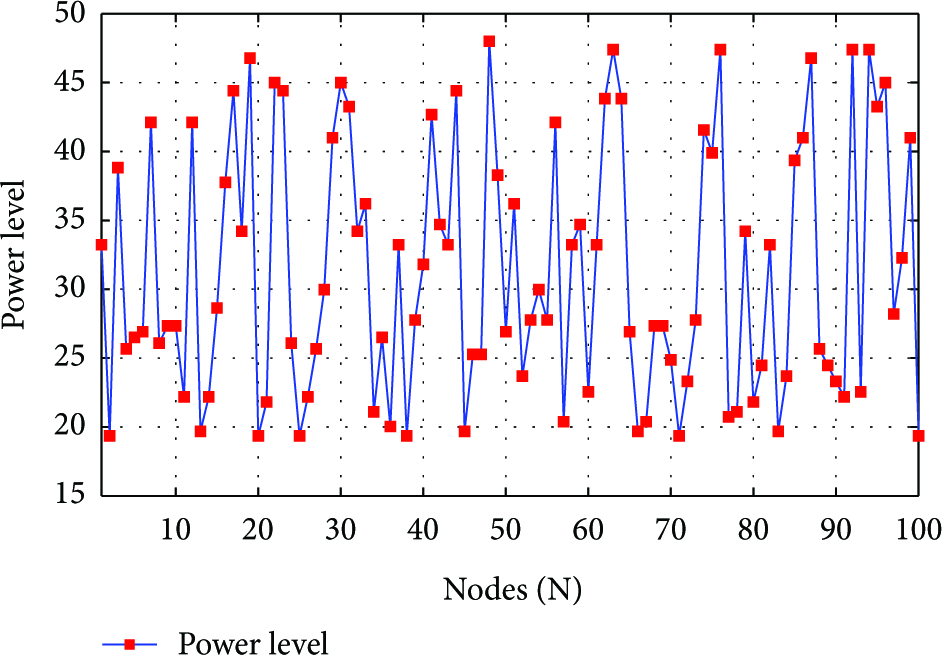
From Figure 4, it is also clear that link quality and $\text{RSS}{\text{I}}_{\text{loss}}$ have inverse relation, when temperature is high $\text{RSS}{\text{I}}_{\text{loss}}$ has high value which means low quality link and vice versa. After estimating $\text{RSS}{\text{I}}_{\text{loss}}$ for each node in WSN, we compute corresponding transmitter $P_{\text{level}}$ to compensate $\text{RSS}{\text{I}}_{\text{loss}}$ . Figure 5 shows the range of $P_{\text{level}}$ on y-axis for given $\text{RSS}{\text{I}}_{\text{loss}}$ , that is, between 20 and 47, and also variation of required $P_{\text{level}}$ for sensor node with changing temperature, that is, at low temperature required $P_{\text{level}}$ is low and for high temperature required $P_{\text{level}}$ is high.

Figure 5

Required power level.

Estimated $\text{RSS}{\text{I}}_{\text{loss}}$ for each sensor node on the basis of given temperature helps to estimate corresponding $P_{\text{level}}$ . That power level only helps to compensate $\text{RSS}{\text{I}}_{\text{loss}}$ due to temperature variations. To compensate path loss due to distance between each sensor node in WSNs, free-space model helps to estimate actual required transmitter power. After the addition of required $P_{\text{level}}$ due to temperature variation and distance, we estimate actual required $P_t$ between each sensor node. Figure 6 shows required $P_t$ including both $\text{RSS}{\text{I}}_{\text{loss}}$ due to temperature variation and free-space path loss for different nodes. We clearly see from figure that $P_t$ lies between −175 and 90, dBm and most of the time it is above −120 dBm.

Figure 6

Transmitter power.

In Figure 7, we have shown $P_{\text{level}}$ using classical approach for three regions and in Figure 8 $P_{\text{level}}$ for the proposed technique, EAST. We can clearly see the difference between $P_{\text{level}}$ assigned. To show $P_{\text{level}}$ for each region, we take the difference between the assigned $P_{\text{level}}$ s using EAST and classical technique, as can be seen in Figures 9, 10, and 11. As we know that in classical approach, there is no concept of subregions, for the sake of comparison with the proposed technique, EAST, we have shown $P_{\text{level}}$ for different regions using classical approach.

Figure 7

Power level using classical approach for regions A, B, and C.

Figure 8

Power level using EAST for regions A, B, and C.

Figure 9

Difference of Power level save between classical technique and EAST for region A.

Figure 10

Difference of power level save between classical technique and EAST for region B.

Figure 11

Difference of power level save between classical technique and EAST for region C.

After estimating $\text{RSS}{\text{I}}_{\text{loss}}$ for nodes of each region, we have estimated required $P_{\text{level}}$ for nodes of each region that we clearly see in Figure 7; in region A, $P_{\text{level}}$ lies 40–45, for region B 30–35 and for region C 20–25. It means that for region A required $P_{\text{level}}$ is higher than both other regions that also shows that for that region temperature and $\text{RSS}{\text{I}}_{\text{loss}}$ are large. For regions B required $P_{\text{level}}$ is between both region A and C, and for C region required $P_{\text{level}}$ is less than both other two regions. We have earlier seen in Figure 7 that $P_{\text{level}}$ for each region is assigned using classical approach. After applying the proposed technique, we see what $P_{\text{level}}$ required for each region. We can clearly see difference from between $P_{\text{level}}$ as shown in Figure 8 that the required $P_{\text{level}}$ decreases for each region and for region A it decrease at its maximum. Figures 9, 10, and 11, respectively, show required $P_{\text{save}}$ for regions A, B, and C after implanting the proposed technique. $P_{\text{save}}$ values reach 2.3 for region A, 1.7 for B and 1.5 for C.

Figure 12 describes the effect of reference node mobility on $P_{\text{save}}$ for region A. Reference node moves around boundaries of square region, and nodes in a region are considered to be static. When a reference node is at center location (50,50) of network, maximum nodes around reference node have large $\text{RSS}{\text{I}}_{\text{loss}}$ than threshold so we need to reduce $P_{\text{level}}$ to meet threshold $P_{\text{level}}$ requirements that cause maximum $P_{\text{save}}$ . We can clearly see maximum $P_{\text{save}}$ 12 dBm to 20 dBm for center location. When a reference node moves from center to one of the corner (0,0) of square region $P_{\text{save}}$ remains constant approximately around 1 dB, because the nodes near reference node having same $\text{RSS}{\text{I}}_{\text{loss}}$ bear constant temperature and they need approximately the same $P_{\text{level}}$ near threshold. $P_{\text{save}}$ for reference node movement from (0,0) to (0,100) fluctuates between −5 dBm and 6 dBm, and at two moments we observe maximum $P_{\text{save}}$ because a number of nodes near reference node have to increase their $P_{\text{level}}$ to meet threshold's minimum.

Figure 12

Transmitter power save in region A for different reference node locations.

Movement of reference node from (0, 100) to (100, 100) causes $P_{\text{save}}$ between −4 dBm and 12 dBm, and only one time peak $P_{\text{save}}$ . Similarly, when a reference node moves from (100, 100) to (100, 0), $P_{\text{save}}$ remains in limits between −4 dBm and 7 dBm, and only one time maximum $P_{\text{save}}$ . From this figure it is also clear that for region A reference node location at center gives maximum $P_{\text{save}}$ that enhances network lifetime. We can also see that variation of $P_{\text{save}}$ depends upon the distance of nodes from reference node, as if nodes have shorter $\text{RSS}{\text{I}}_{\text{loss}}$ than threshold, then we have to increase $P_{\text{level}}$ that enhances $P_{\text{save}}$ and vice versa. It is also clear from result that peak maximum and minimum $P_{\text{save}}$ comes at a same time.

Similarly we can see $P_{\text{save}}$ for similar pattern of reference node mobility considering regions B and C. For region B in Figure 13 when reference node at center location (50, 50) $P_{\text{save}}$ remains between 14 dBm and 20 dBm, from center to (0, 0) $P_{\text{save}}$ remains between 0 and 1dBm. When a reference node moves from (0, 0) to one of the corner of square regions (0, 100) $P_{\text{save}}$ fluctuates between 0 and 4 dBm. Reference node's movement from (0, 100) to (100, 100) causes $P_{\text{save}}$   to change from  1 dBm to 5 dBm and from (100, 100) to (100, 0) increases $P_{\text{save}}$ change from 4 dBm to 5 dBm.

Figure 13

Transmitter power save in region B for different reference node locations.

This figure also indicates that $P_{\text{save}}$ for region B is maximum when a reference node is at center location. For reference node mobility from center to (0, 0), $P_{\text{save}}$ remains constant due to constant $\text{RSS}{\text{I}}_{\text{loss}}$ near reference node region. For other reference node movements, $P_{\text{save}}$ remains approximately constant due to less variations in $\text{RSS}{\text{I}}_{\text{loss}}$ . Compared to region A where $P_{\text{save}}$ goes to peak maximum and minimum values in region B, $P_{\text{save}}$ remains on average approximately constant and less variation occurs; fact is that nodes in region B have approximately the same $\text{RSS}{\text{I}}_{\text{loss}}$ near threshold.

$P_{\text{save}}$ for reference node mobility in region C around square is shown in Figure 14. When a reference node is at center (50, 50), $P_{\text{save}}$ fluctuates between 8 dBm and 50 dBm. From center to edge (0, 0), reference node mobility causes $P_{\text{save}}$ around 0 dBm. When a reference node moves from a corner of square (0, 0) to corner (0, 100), $P_{\text{save}}$ −5 dBm–12 dBm. Similarly from (0, 100) to (100, 100), $P_{\text{save}}$ remains between −10 dBm and 18 dBm. Finally when the reference node is location changes from (100, 100) to (100, 0) and $P_{\text{save}}$ goes to maximum value 60 dBm that shows that nodes near reference node have larger $\text{RSS}{\text{I}}_{\text{loss}}$ than threshold $\text{RSS}{\text{I}}_{\text{loss}}$ at that moment. Figures 12, 13, and 14 also elaborate that on average $P_{\text{save}}$ is maximum for reference node location at center. Compared to region B, in this region peak maximum and minimum $P_{\text{save}}$ exists the reason is that nodes in this region have larger $\text{RSS}{\text{I}}_{\text{loss}}$ than threshold at that moment.

Figure 14

Transmitter power save in region C for different reference node locations.

6. Conclusion and Future Work

In this paper, we presented a new proposed technique, EAST. It shows that temperature is one of the most important factors impacting link quality. Relationship between $\text{RSS}{\text{I}}_{\text{loss}}$ and temperature has been analyzed for our transmission power control scheme. The proposed scheme uses open-loop control to compensate for changes of link quality according to temperature variation. By combining both open-loop temperature-aware compensation and close-loop feedback control, we can significantly reduce overhead of transmission power control in WSN; we further extended our scheme by dividing network into three regions on basis of threshold $\text{RSS}{\text{I}}_{\text{loss}}$ and assigned $P_{\text{level}}$ to each node in three regions on the basis of current number of nodes and the desired number of nodes, which helps to adapt $P_t$ according to link quality variation and increase network lifetime. We have also evaluated the performance of the proposed scheme for reference node mobility around square region that shows $P_{\text{save}}$ up to 60 dBm. But in case of static reference node, $P_{\text{save}}$ goes maximum to 2 dBm.

In future, firstly, we are interested to work on Internet Protocol (IP) based solutions in WSNs [14]. Secondly, as sensors are usually deployed in potentially adverse environments [15], we will address the security challenges using the intrusion detection systems because they provide a necessary layer for the protection.