Sage Journals: Discover world-class research

Abstract

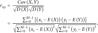
Wireless sensor networks (WSNs) have limited energy and transmission capacity, so data compression techniques have extensive applications. A sensor node with multiple sensing units is called a multimodal or multivariate node. For multivariate stream on a sensor node, some data streams are elected as the base functions according to the correlation coefficient matrix, and the other streams from the same node can be expressed in relation to one of these base functions using linear regression. By designing an incremental algorithm for computing regression coefficients, a multivariate data compression scheme based on self-adaptive regression with infinite norm error bound for WSNs is proposed. According to error bounds and compression incomes, the self-adaption means that the proposed algorithms make decisions automatically to transmit raw data or regression coefficients, and to select the number of data involved in regression. The algorithms in the scheme can simultaneously explore the temporal and multivariate correlations among the sensory data. Theoretically and experimentally, it is concluded that the proposed algorithms can effectively exploit the correlations on the same sensor node and achieve significant reduction in data transmission. Furthermore, the algorithms perform consistently well even when multivariate stream data correlations are less obvious or non-stationary.

1. Introduction

Wireless sensor networks (WSNs) can monitor, sense, and collect the data of various environments or monitored objects in an area. And the data are eventually sent to the target users [1]. WSNs have wide range of potential applications including home area and smart grid [2]. Each sensor node in WSN has limited battery power supply, and the used batteries are hard to recharge and replace. It is infeasible that a large number of nodes directly transmit the collected raw data to the base station or sink due to limited bandwidth and battery capacity. Wireless communication consumes most of the power. The literature [3] shows that the power consumed by transmitting the 1-bit data over a 100-meter distance can support to execute 3000 CPU instructions. The literature [4] also points out that the power consumption of the data transmission is much higher than that of data processing. Transmitting a 1-bit data via radio medium is at least 480 times the power consumption used for executing one “addition” operation. Approximately, 70% of the total power is consumed in data transmission. How to effectively reduce the amount of data within the WSN in order to extend the network lifetime is an important issue. Sensor energy can be saved via mechanisms at different layers of the WSN protocol stack [5–8], such as energy efficient routing [9] and battery saving media access control [10], where there are plenty of existing work. L. Zhang and Y. Zhang [11] presented an energy-efficient packet forwarding protocol in wireless sensor networks, considering channel awareness and geographic information. The perspective of this paper is from the application layer by introducing effective data compression.

Sensor nodes use the data sensing units to collect raw data and then transmit the data processed through the data processing units to reduce the amount of data to be transmitted. Generally, there are two types of processing methods [12]: data aggregation and data approximation. Aggregate functions process the sampled data using some forms of simple statistics such as maximum, minimum, and average. It is an effective mean to reduce the volume of data. However, it just provides simple coarse statistical information while potentially hiding some interesting local varieties of the data. Data approximation can be regarded as a model-based data processing method. When data feeds exhibit a large degree of redundancy, approximation is a less intrusive form of data reduction in which the underlying data feed is replaced by an approximate signal tailored to the application needs. It is only required to transmit the parameters of the distributed model built for the sensor data collected from WSN. Thereby, the amount of transmitted data is greatly reduced, resulting in network energy being saved, and thus the network lifetime is being prolonged. In terms of the way they are applied, there are four major categories for data approximation: probabilistic model [13, 14], time series analysis model [15–17], data mining model [18], and data compression model [19–24].

The paper is based on the following three facts which also show the application scenario. (1) Multivariate correlation exists. With the development of the wireless communication and microelectronics technology, wireless sensor node equipped with several sensing units has become popular. Such node can simultaneously monitor several types of data, such as sound intensity, acceleration, temperature, humidity, light intensity, and video, in which certain correlation universally exists. In this paper, the data collected by different sensing units in the same sensor node are referred to as multivariate data or multiattribute data, and the correlation among these different data type is called multivariate correlation or multiattribute correlation. (2) Spatial correlation does not exist. Most distributed compression algorithms are based on the assumption that nodes have spatial correlations with other nodes. This introduces large implementation cost. In real life, people often hope to use as small number of sensor nodes to monitor as wide an area as possible in order to reduce investment cost. As a result, these nodes are placed far away from each other, leading to no or little of unstable spatial correlation. In this case, it is a better choice that the algorithm is designed to run independently on each node. (3) Error is bounded. Influencing by noise, node failure, unreliable wireless communication, power constraints, and other factors, it exists certain error in acquisition, processing, and transmission processes of sensor data. The sensor data has a certain degree of uncertainty. If the user does not need very accurate results, by sacrificing the data precision, he can achieve the purpose of reducing the data amount of communication. Our study is devoted to minimize the volume of the transmitted data in the error bound predefined by the user.

The major contribution of the paper lies in the following aspects. This paper designs the algorithms considering the temporal and multivariate correlations of the data and also taking into account the case when the multivariate correlation is unstable, but without considering the spatial correlation of the data. Our algorithms run in each sensor node collecting a number of data streams. This paper proposes a self-adaptive regression-based multivariate data compression algorithm with error bound (denoted as AR-MWCEB) and implements it in C. According to the predetermined error bounds, AR-MWCEB makes decision automatically to transmit raw data or regression coefficients and to select the number of data involved in each regression. The results of simulation experiments show that the algorithm can reduce the amount of transmitted data and has better real-time performance than the benchmark algorithms.

The rest of the paper is organized as follows. Section 2 describes the related work, which is followed by the introduction of some preliminary knowledge and the problem formulation in Section 3. Section 4 presents the proposed compression scheme, base selection algorithm, and incremental calculation of regression coefficient. A self-adaptive regression-based multivariate data compression algorithm with error bound is detailed in Section 5. After the presentation of the intensive simulation results and performance analysis in Section 6, the paper is concluded in Section 7.

2. Related Work

Multivariate streams measured from one sensor node are correlated. The same is often true in other domain. Deligiannakis et al. [12] pointed out that the scatter diagram with indexes of industry and insurance from the New York stock market as the x-axis and y-axis coordinates, respectively, appears to be an approximated straight line. Each original time series is not linear, but he proposed a SBR algorithm using the base signal as an independent variable and the regression model to piecewise approximate other series. The values of the base signal are extracted from the real measurements and maintained dynamically as data changes. When the multivariate correlation measured by a sensor node is larger, this algorithm is better. But SBR algorithm does not consider the problem of error bound, and it just compresses data in the maximum degree under satisfying the condition of data compression. It may lead to two problems: (1) the algorithm is terminated before the error margin reaches its predetermined requirement; (2) the data is still continuously compressed when the error has met the requirement.

For the data generated by the single sensor node, the RACE algorithm [19] proposes a Haar wavelet compression algorithm with adaptive bit rate. It can output CBR (constant bit rate) or LBR (limited bit rate) streams by selecting the significant wavelet coefficients based on a threshold. RACE runs on a single node. In spite of reducing the transmission of redundant data by eliminating the temporal correlation, it does not consider the spatial correlation among neighboring nodes or multiattribute correlation in the same node. Ciancio et al. [20] study a distributed wavelet compression algorithm, which exchanges information among neighboring nodes and distributes the discovered spatial correlation of the sensor network data before the data are transmitted to the sink node. Although the algorithm has greatly reduced the transmission of redundant data, however, information exchange among nodes would result in some cost, such as power consumption and network delay, which needs further quantitative analysis in theory.

The literature [21] designs a new algorithm based on multiattribute correlation. The algorithm can effectively reduce spatial, temporal, and multivariate correlations, but there are two problems limiting its performance. (1) All the raw data of each node in a cluster must be sent directly to the cluster head and must be processed in the cluster head. The data with different attributes but from different nodes are not differentiated, but rather they are abstracted into a column of the processed data matrix. (2) Before sending data, the cluster head must call data preprocessing algorithm to analyze and find out the attribute pairs between which the correlation is large. In this processing, the estimated attribute data are fitted using the least square method. Our previous algorithms proposed in [22] run independently in each of the sensor nodes, and no collaboration exists between nodes. It uses the single data stream wavelet compression algorithm with error bound (SWCEB) to do wavelet decomposition to the maximum level resulting in full elimination of the temporal correlation of the data to satisfy the error bound in the coefficient selection. Meanwhile, it eliminates multiattribute correlations and uses the regression-based multiple data streams wavelet compression algorithm with error bound (MWCEB), in which the regression intervals are continuously bisected if needed to ensure that the error is bounded. The binary partition is arbitrary, so this paper will try to self-adaptively determine the number of data involved in each regression calculation.

It is worth mentioning that both multiple data streams (the data streams collected by a cluster head from all other nodes in the cluster) [23] and multiattribute data stream (the data streams collected by the single sensor node having multiple sensing units) can be effectively compressed by our proposed AR-MWCEB scheme. Furthermore, after the multiple data streams being processed by the cluster head, its spatial correlation is reduced, and after the multiattribute data stream is being processed in the multimodal node, its multivariate correlation is also reduced. This paper focuses on reducing the multivariate correlation of multiattribute data stream, but the result can also improve the performance of DLRDG [23].

Sadler and Martonosi [24] propose a lossless compression algorithm for sensor nodes in WSNs, called S-LZW. They discuss some design problems in detail about implementation, adaptability improvement, customizing compression techniques, and so on. Research on lossless data compression in WSNs is still in its early stage with very few published papers.

3. Preliminaries and Problem Statement

Many monitoring data collected by sensor nodes such as temperature, humidity, light, and vibration always slightly varies within a continuous time, and most of successive data are the same or similar. When these successive data are decomposed by wavelet transform, the majority of the energy is concentrated in the low-frequency coefficients. High-frequency coefficients are 0 or close to 0. Even if the monitored object changes abnormally, which causes unusual fluctuations of sensor data, the multiresolution characteristic of the wavelet transform can ease the impact of these unusual fluctuations on the overall data. It maintains values of some detail components as approximately 0. Compressing (discarding) the detail components with value 0 does not affect the data reconstruction; compressing the nonzero detail components would affect the data accuracy. The more detail components are compressed, the higher the compression ratio of the data is, but the larger the caused data error is. Therefore, under the premise of guarantee of error bound, detail components should be compressed maximally.

The distributed wavelet compression algorithm for the sensor networks is designed to complete the task by multiple nodes together. In this algorithm, the wavelet transform is calculated dispersedly in each node, and the wavelet coefficients are also dispersed at each node. Thereby, the amount of calculation for each node is small. The performance of using two-level wavelet transform is slightly better than that of using single-level transform, because the second level of the wavelet transform can better eliminate the correlation, in spite of increasing the additional energy consumption and time delay. Communication overhead and time delay are increased constantly with increasing the level of wavelet decomposition; thus, the distributed compression algorithm cannot always rely on increasing the wavelet decomposition level to improve its performance. Our algorithm runs independently on each sensor node, there is no collaboration among nodes; therefore, wavelet transform can decomposes the data with the maximum level to eliminate the temporal correlation of enough data.

Garofalakis and Gibbons [25] firstly proposed a wavelet-based compression technique with error guarantees of data reconstruction by introducing probabilistic wavelet synopses. Based on the error tree from the literatures [25, 26], a single-attribute data wavelet compression algorithm with error bound named SWCEB is proposed by us in the literature [22]. It includes four steps: wavelet decomposition, coefficient selection, quantization, and entropy coding. In the step of coefficient selection, it guarantees to satisfy the error bound. And it eliminates the temporal correlation in a single data stream through Haar wavelet transform. Furthermore, literature [22] proposes a multiattribute data compression algorithm with error bound named MWCEB, which is based on regression and divided into three steps: (i)

selecting some attributes as the base attributes according to the correlation coefficient matrix of multiattribute sampling data;

(ii)

using SWCEB algorithm to compress the base attributes data;

(iii)

describing other nonbase attributes data by linear regression coefficients of one of the base attributes.

MWCEB algorithm can guarantee the satisfaction of error bound by increasing the number of base attributes. However, in the worst case, it degenerates into the SWCEB algorithm without taking advantage of multiattribute correlation. Another way to reduce error for MWCEB algorithm is to reduce the number of data involved in the regression calculation, that is, to carry out piecewise linear regression. As MWCEB algorithm arbitrarily divides the regression intervals equally without considering the data correlation, its processing parameters required manual intervention, and its regression performance is not ideal.

Within the framework of the above processing procedure, this paper tries to self-adaptively determine the number of data involved in the regression calculation each time to guarantee that the error is bounded. If successive data is a dramatic change, it is difficult to use a linear regression model to describe the nonbase attribute. Thus, the self-adaptive piecewise linear regression which automatically determines the data number involved in the regression calculation each time or direct transmission of the raw sampling data is selected automatically.

Assuming the data buffer size of a sensor node is M, the collected data is denoted as $s [0], \dots, s [M - 1]$ , and the reconstructed approximation data is $s^{*} [0], \dots, s^{*} [M - 1]$ . Dealing with multiattribute data, it usually uses normalized infinite norm error.

Definition 1 (normalization of the sampling data).

$s [i]$ is normalized to $norm (s [i]) = (s [i] - s_{\min}) / (s_{\max} - s_{\min})$ , where $s_{\max}$ and $s_{\min}$ are the maximum and minimum values of the sampling data collected in a period, respectively. Obviously, the value of $norm (s [i])$ is located in $[0, 1]$ . When dealing with multiattribute data, the normalization of sampling data can prevent the attribute with small amplitude being concealed by the ones with large amplitude.

Definition 2 (normalization error).

$e_{i}^{norm} = | norm (s [i]) - norm (s^{*} [i]) |$ .

Definition 3 (∞-norm average error).

${∥ e ∥}_{\infty} = \max_{0 \leq i < M} | s [i] - s^{*} [i] |$ . ∞-norm average error bound guarantees the error bound of each reconstructed data and the corresponding sampling data. The normalized infinite norm average error is defined as ${∥ e ∥}_{_{\infty}}^{norm} = (\max_{0 \leq i < M} | s [i] - s^{*} [i] |) / (s_{\max} - s_{\min})$ .

Definition 4 (the correlation coefficient matrix).

M times samples $x_{i}$ , $i = 0 \dots M - 1$ of an attribute can be recognized as M times experiments of a discrete random variable X. The relationship between the attributes X and Y can be measured by the correlation coefficient, which is defined as follows:

\begin{matrix} r_{x y} = \frac{Cov (X, Y)}{\sqrt{D (X)} \sqrt{D (Y)}} \\ = \frac{\sum_{i = 0}^{M - 1} [(x_{i} - E (X)) (y_{i} - E (Y))]}{\sqrt{\sum_{i = 0}^{M - 1} {(x_{i} - E (X))}^{2}} \sqrt{\sum_{i = 0}^{M - 1} {(y_{i} - E (Y))}^{2}}}, \end{matrix}

(1)

where

E (X) = \sum_{i} p_{i} x_{i} = (1 / M) \sum_{i = 0}^{M - 1} x_{i}

. If X and Y are positive (negative) correlations, r is positive (negative); when

r = 1 (- 1)

, their relationship is complete positive (negative) correlation, and all the data points lie on the regression line. The more scattered the data points are, the smaller the absolute value of r is, and the lower the correlation is. If each node can collect N attributes, the correlation coefficient matrix R with the size

N \times N

is defined to express the relationship among all attributes, in which the element of the jth column in the ith row represents correlation coefficient between the ith and the jth attributes.

Definition 5 (the best correlation of attribute $X_{j}$ for the base attributes set).

Suppose that N attributes streams $X_{0}$ , $X_{1}, \dots$ , $X_{N - 1}$ have some correlations, and that they have been classified into the base attributes set BaseSet and the candidate attributes set CandSet, where the index used in both sets represents the corresponding stream. The best correlation between the element $X_{j}$ in CandSet and all of the elements in BaseSet is defined as follows:

\begin{matrix} {b e s t f i t}_{j} = \max_{i} (| r_{i j} |), i \in B a s e S e t . \end{matrix}

(2)

Then, an element

X_{j}

in CandSet can be represented by regression coefficients of using the element

X_{i}

(recorded in variable

p o s i t i o n_{j}

) in BaseSet, in the condition that the absolute value of the correlation coefficient between these two elements is the largest. If the error is too large, the element would move to BaseSet. Obviously, the best correlation of the elements in the base attributes set is 1.

Definition 6 (the expected income of adding candidate attribute $X_{j}$ to the base attributes set).

The N attributes are divided into the base attributes set BaseSet and the candidate attributes set CandSet. If attribute $X_{j}$ is added to BaseSet, the expected income is defined as:

\begin{matrix} {i n c o m e}_{j} = \sum_{k} (| r_{j k} | - {b e s t f i t}_{k}), \\ k \in {k \in C a n d S e t \land | r_{j k} | > {b e s t f i t}_{k}} . \end{matrix}

(3)

Initially, CandSet contains N attributes, and BaseSet is empty. After summing the absolute value of the elements in the correlation coefficient matrix row by row, choose the attribute corresponding to the maximum sum and add it to BaseSet as a base. Then, according to error bound, decide if you will continue to look for other bases. In the process of each base selection, add the

X_{j}

from CandSet with the largest expected income to BaseSet; at the same time, update

{b e s t f i t}_{i}

of the remaining attribute

X_{i}

in CandSet, and correspondingly update

{p o s i t i o n}_{i}

to express that we regress the

X_{i}

in CandSet on the

X_{j}

in BaseSet.

4. Base Selection and Coefficient Incremental Calculation for Regression

4.1. Base Selection and Linear Regression

Suppose that a sensor node has N sensing units, and the collected attribute is $A_{j}$ , $j = 1,2, \dots, N$ . The overall operation of the regression-based compression scheme is as follows.

Step 1.

Using our base selection algorithm proposed in [22], classify all attributes into several groups $G_{i}$ , $i = 1, 2, \dots, K$ , according to their correlation coefficient matrix. $⋃_{i = 1}^{K} G_{i} = ⋃_{j = 1}^{N} A_{j}$ and for all $i \neq j, G_{i} ⋂ G_{j} = \emptyset$ . The attributes with large correlation are located in the same group. Definitions 5 and 6 in Section 3 have implicitly described our base selection method. The base selection algorithm can also be implemented by consulting the K-Means and other clustering algorithms.

Each group $G_{i}$ , $i = 1, 2, \dots, K$ , has only one base attribute, and other attributes in the same group are represented by the base and linear regression coefficients. For the convenience of description, denote the selected base in a group as attribute X and a nonbase attribute located in the same group with attribute X as attribute Y. The attribute Y can be represented by several regression coefficient pairs generated by linear regression.

Step 2.

Run the SWCEB algorithm on M sampling data of the base attribute X. After wavelet decomposition, set some wavelet coefficients to 0 in the case of error bound. The local reconstructed data by wavelet transform is directly used as the base signal X of the regression. As a result, it avoids to spread the base reconstruction error to other nonbase attributes, and the reconstructed base signal is more regular and more suitable for use as a base than the original one.

Step 3.

Regress the nonbase attributes on the base attribute from the group in which the nonbase attributes locate, and transmit the calculated regression coefficients. The raw data of the nonbase attributes is no longer required to be transmitted.

The implementation of Step 3 is analyzed below in details. When the estimation of nonbase attribute Y is $\tilde{Y} = a X + b$ , find the regression coefficients a and b so that $| | Y - \tilde{Y} | |_{2}$ is minimum; namely, minimize the objective function $Q = \sum_{i} (y_{i} - a x_{i} - b)^{2}$ . When

\begin{matrix} \frac{\partial Q}{\partial a} = 0, \frac{\partial Q}{\partial b} = 0 \end{matrix}

(4)

solve the linear equations with two unknowns

\begin{matrix} \sum_{i} (y_{i} - a x_{i} - b) (- x_{i}) = 0, \\ \sum_{i} (y_{i} - a x_{i} - b) (- 1) = 0, \end{matrix}

(5)

to find a, b.

Then,

\begin{matrix} a = \frac{M * \sum_{i = 1}^{M} (x_{i} * y_{i}) - \sum_{i = 1}^{M} x_{i} * \sum_{i = 1}^{M} y_{i}}{M * \sum_{i = 1}^{M} x_{i}^{2} - {(\sum_{i = 1}^{M} x_{i})}^{2}}, \\ b = \frac{\sum_{i = 1}^{M} y_{i} - a * \sum_{i = 1}^{M} x_{i}}{M} . \end{matrix}

(6)

In this way, a candidate attribute can be represented by a pair of regression coefficients. The base attribute is compressed by Haar wavelet in Step 2, and the number of data being processed each time is some power of 2. It is worth noting that the more the number of data is involved in each regression, the bigger the regression error is. According to the number M of the processed data each time, our proposed MWCEB algorithm employs the piecewise linear regression with the equal number of data (obviously, this will lead to a large error), and simply transmits the regression coefficients a and b. If

M = 2

, then the regression would not cause any compression; furthermore, in order to achieve the convenience of wavelet compression of the selected base, the number of data is also preferable to be as some power of 2, so the number of processed data in each time should be 4 at least.

4.2. Incremental Calculation for Regression

Now, we will introduce how to use self-adaptive regression to make decisions automatically to transmit raw data or regression coefficients, and how to automatically obtain the number of the data involved in each regression calculation. The number of data in each regression is set to some power of 2 for convenience. If the regression results satisfy the error bound, the start number start and the count number length of the data participating in the regression should be transmitted, as well as the regression coefficients a and b. If $l e n g t h = 4$ , then the regression would not cause any compression, so length should be greater than or equal to 8. If the regression results of 8 (or some power of 2 greater than 8) data satisfy the error bound, only 4 data on representation of regression results need to be transmitted; Otherwise, the raw sampling data is directly transmitted. In order to obtain the best compression performance, length is doubled constantly until find the maximum number of regressed data in the condition of error bound.

Through analyzing the equations of calculating the regression coefficients a and b, it is found that the regression coefficients can be incrementally calculated. Define a data structure as in Algorithm 1.

Algorithm 1:

(1) typedef struct {

(2) double sum_x;

(3) double sum_xx;

(4) double sum_xy;

(5) double sum_y;

(6) }COEFF;

(7) COEFF coeff, firsthalf_coeff, *pcoeff;

The AuxCalc is an auxiliary function used by the incremental regression, which is implemented as in Algorithm 2.

Algorithm 2: The AuxCalc function.

(1) Function AuxCalc(int start , int length COEFF * pcoeff )

(2) input: the sampling data of related attributes X[start ⋯ start+length-1], Y[start ⋯ start+length-1]

(3) output: coeff

(4) begin

(5) pcoeff ->sum_x=0;

(6) pcoeff->sum_xx=0;

(7) pcoeff->sum_xy=0;

(8) pcoeff->sum_y=0;

(9) for i=start to start+length-1 {

(10) pcoeff->sum_x += X[i];

(11) pcoeff->sum_xx += X[i]*X[i];

(12) pcoeff->sum_xy += X[i]*Y[i];

(13) pcoeff->sum_y += Y[i]; }

(14) end

When the regression results satisfy the error bound condition, the number of regressed data length is doubled repeatedly for exploring the maximum length. Known by analysis of (6), when length is increased to 2 times of the raw one, the calculated coeff in the previous regression calculation can still be effectively used. Therefore, they can be saved as a static variable or global variable firsthalf_coeff for the use in the next regression calculation. In addition, assignment operators for the variables of COEFF type can be implemented by the addition and assignment of each corresponding fields.

The incremental calculation function of regression coefficients is described as in Algorithm 3.

Algorithm 3: The IncRegress function.

(1) Function IncRegress(int start , int length , double eps , double * a , double * b , int * cnterr )

(2) input: the predefined regression error bound eps; the sampling data of related attributes X[start ⋯ start+length-1],

Y[start.. start+length-1]

(3) output: the regression coefficients a and b; the number errcnt of data exceeding the error bound

(4) begin

(5) if length==8 then

(6) AuxCalc (start, length, &coeff);

(7) else{

(8) AuxCalc (start+ length/2, length/2, &coeff); // length/2 data does not need to be summed once again

(9) coeff+= firsthalf_coeff; }

(10) firsthalf_coeff= coeff;

(11) *a= (length*coeff.sum_xy - coeff.sum_x*coeff.sum_y)/(length*coeff.sum_xx - coeff.sum_x*coeff.sum_x);

(12) *b= (coeff.sum_y - *a*coeff.sum_x)/length; // recursive form of (6)

(13) *cnterr = 0;

(14) double max_y=−32768, min_y = 32767;

(15) for i=0 to M-1{

(16) if max_y < Y[i] then max_y= Y[i];

(17) if min_y > Y[i] then min_y=Y[i]; }

(18) for i=start to start+length-1{

(19) if fabs(*a*X[i]+ *b-Y[i])> eps*(max_y - min_y) then (*cnterr)++; }

(20) end

5. A Self-Adaptive Regression-Based Multivariate Data Compression Algorithm with Error Bound

5.1. The Proposed Algorithm

The proposed self-adaptive regression-based multivariate data wavelet compression scheme with error bound is abbreviated to AR-MWCEB. Its basic idea is as follows. (1) Calculate the regression error of the first 8 being processed data in the buffer of a sensor node. (2) If the calculated regression error does not satisfy the predefined error bound, transmit directly these 8 raw data, or else, and recalculate the regression error after doubling the number of regressed data until that the maximum number of the regressed data with satisfaction of the predefined error bound is found in order to obtain the best compression performance. In this case, it only needs to transmit 4 data that described the regression process to represent one segment of the raw sampling data of the nonbase attribute. (3) repeat the above process starting from the first unprocessed data to the last one.

Assuming that the number of the regressed data is l and the error bound is satisfied, but the error bound is not satisfied when it is $2 * l$ . Comprehensively considering the convenience of calculation, the computation complexity, the storage capacity, and so forth, the regression with $l + 1$ to $2 * l - 1$ data is not been explored calculation. The new segment to be processed directly starts from $l + 1$ after transmitting the regression representation of the l data.

The compression algorithm based on self-adaptive regression is described as in Algorithm 4.

Algorithm 4: The AR-MWCEB algorithm.

(1) Function AdapRegressCompress(double eps , int start , int size )

(2) input: the predefined regression error bound eps denoted by the average error of normalized infinite norm;

the sampling data of related attributes X[0 ⋯ M−1], Y[0 ⋯ M−1], M is the number of buffer data in a sensor node;

initially start is 0 and size is M.

(3) output: the compression representation of non-base attribute Y, in the receiving end which can be used to

reconstruct the raw sampling data satisfied the predefined regression error bound

(4) begin

(5) double a, b, old_a, old_b;

(6) int counterror;

(7) loop:

(8) int startpos= start;

(9) int count= 8;

(10) while (startpos+ count <= start+ size) do{

(11) IncRegress (startpos, count, eps, &a, &b, &counterror);

(12) if (counterror> 0) then{

(13) if (count==8) then{

(14) Directly transmit the eight raw data Y[startpos ⋯ startpos+7] to the receiving sensor node;

(15) startpos += 8; }

(16) else{

(17) Transmit the 4-tuples (old_a, old_b, startpos, count/2) for regression representation of count/2 data;

(18) //the approximation of Y[startpos.. startpos+count/2-1] can be reconstructed by the 4-tuples

in the receiving end

(19) startpos += count/2;

(20) count=8; }

(21) }

(22) else {

(23) count*= 2;

(24) old_a= a;

(25) old_b= b; }

(26) } //end while

(27) if (startpos!= M) then {

(28) Transmit the 4-tuples (old_a, old_b, startpos, count/2) for regression representation of count/2 data;

(29) start= startpos+ count/2;

(30) size= M - start;

(31) if (size) then AdapRegressCompress (eps, start, size);

(32) //The above statement can also been expressed as: if (size) then goto loop;

(33) } //end if

(34) end

5.2. Properties of the Algorithm

Property 1.

After transmitting the part of the data each time, the number of the remaining data shall be a multiple of 8.

Proof.

We assume that the size M of the data buffer in a sensor node is some power of 2. This assumption accords with the actual situation of the memory hardware, and it is also convenient for making wavelet transform on the base attribute in Step 2 of Section 4.2. The total number of data of each attribute in a buffer is usually some power of 2 and more than 2¹⁰. Set it to $2^{3} * 2^{x}$ ; namely, it is $8 X$ , where X is a natural number. Algorithm 3 either directly transmits 8 raw data or transmits 4 tuples to represent 8 (or 8 multiplying by some power of 2) raw data; that is, the number of processed raw data each time is also a multiple of 8, denoted as $8 Y$ , where Y is a natural number. Therefore, $8 (X - Y)$ raw data are left after processing a part of the data each time; that is, the number of remaining data in the buffer must be a multiple of 8.

Property 2.

AdapRegressCompress algorithm complying with the aforementioned process is correct.

Proof.

When the condition of the while loop in line 10 of AdapRegressCompress algorithm is true, the codes within the loop body are executed. However, only one of three cases can be executed in each loop. The three cases are (1) if the conditions in both line 12 and line 13 are true, the block statement from lines 14 to 15 will be executed; (2) if the condition in line 12 is true but the condition in line 13 is false, the block statement from lines 17 to 20 will be executed; (3) if the condition in line 12 is false, the block statement from lines 23 to 25 will be executed.

The values of variables start and size are kept unchanged in the process of repeatedly executing the loop body. For each loop, if some data are transmitted, then the increment of variable startpos is 8 at least; if no data are transmitted, then the value of variable count is doubled. Thus, the while loop must be terminated after finite loops. Next, analyze the states of terminating the while loop by the three cases, respectively. (1)

If the while loop is terminated after execution of line 15. The number of remaining data is a multiple of 8 according to Property 1. After executing statement 15, only 8 data are processed. Now, the loop condition is no longer satisfied; it has shown that only 8 data are left before this loop, and this loop happens to deal with all data. At this time, startpos equals to M. The algorithm ends.

(2)

If the while loop is terminated after execution of line 20. Denote startpos, count as startpos1, count1 and startpos2, and count2 before and after this loop, respectively. Because count1 ≠8, then count1 16. So startpos1 + count1 = startpos1 + count1/2 +count1/2 = startpos2 + count1/2 startpos2 + 8 = startpos2 + count2. As the condition startpos1 + count1 ≤start + size is true when statement 17 is executed, then startpos2 + count2 ≤start + size, and this loop must be executed once after executing statement 20; that is, the while loop cannot be terminated by the second case.

(3)

If the while loop is terminated after execution of line 25. Lines 27 to 33 deal with the third case. At this time, the first count/2 data can be represented by regression model, and only 4 tuples need to be transmitted. With the statement 29 and 30, the starting position and the number of the remaining data are calculated. If there are still some remainder data unprocessed, the above process can be repeated by the goto statement in line 32. A more intuitive expression is to recursively invoke this algorithm, namely, the statement 31.

5.3. Complexity Analysis of the Algorithm

The body of AdapRegressCompress algorithm mainly includes a while loop. In addition to the while loop, statement 11 and statement 31 are the two most time-consuming operations. Similar to the extreme cases of the three terminations of the while loop in previous correctness analysis, the average performance of AdapRegressCompress falls into the range among these extreme cases.

(1) When the linear correlation between the M data and the data of the base attribute is small, 8 raw data must be transmitted each time resulting in no compression. Each raw data is just used one time (i.e., in statement 11) according to AuxCalc. The time complexity is the least. The while loop from statements 10 to 26 must be executed $M / 8$ cycles before termination, and statements 27 to 33 will not be carried out.

(2) Set $M = 2^{m + 3}$ to represent the raw data is divided into $2^{m}$ segments, each containing 8 data. As shown in Figure 1(a), when 8 data satisfy the error bound, but 16 data do not in each regression, the compressed data size is half of the raw one. In Figure 1, 8 segments are given for illustrations, and the horizontal line in each row represents the interval of the raw data involved in regression before transmitting data each time. The first cycle of the while loop uses the first segment with the conclusion that the regression error bound is satisfied. Then the second cycle is followed to be executed after doubling the regression interval to 16 data. Now, the processed 16 data do not satisfy the error bound, and then transmit the representation of the first 8 data with regression coefficients. However, statement 11 has to be executed on 8 data in the second segment again. Except that the 8 data in the first segment are just passed to AuxCalc one time for calculation, all the remaining $M - 8$ are required to be used twice by AuxCalc, whose time complexity is the largest. The while loop from statements 10 to 26 must be executed $M / 4 - 1$ cycles before termination, and statements 27 to 33 will not be done.

Figure 1

Illustration of data segments involved in regression.

As shown in Figure 1(b), when calculation with the first half part of the processed data in each time satisfies the error bound, but with the whole data does not, its compression performance is better than that of the left subgraph. The number of data used by AuxCalc is $8 * 2^{m} + 8 * 2^{m - 1} + \dots + 8 = 2 M - 8$ , the same as the case of the left subgraph. The while loop from statements 10 to 26 must be executed $(m + 1) + (m) + \dots + 1 = m (m + 1) / 2$ cycles to be terminated, and statements 27 to 33 will not be done.

(3) When all the M data are satisfied the regression error bound, the compression performance is best. Each data is simply used once in AuxCalc, its time complexity is the smallest. The while loop with statements 10 to 26 must be executed $m + 1 = \log_{2} M - 2$ cycles to be terminated, and statements 27 to 33 need to be done once, while the condition in statement 31 is not satisfied.

6. Experiments

The used dataset is provided by Samuel Madden et al. (http://db.csail.mit.edu/labdata/labdata.html), containing more than 2.30 million data collected by 54 Mica2Dot nodes at the same time. Each Mica2Dot node collects four kinds of attribute data: temperature, humidity, light intensity, and voltage, denoted as attributes no. 0, no. 1, no. 2, and no. 3, respectively.

Each real number such as sampling data, wavelet coefficient, regression coefficient, which is stored in Micaz nodes, needs 2 bytes for storage. 2 bytes are enough for storing an integer such as start number start and the count number length of data. The number of samples in a sensor node buffer is usually no more than $4 K$ in order to prevent too long time delay; thus the variable start and length can be totally stored by 3 bytes. The proposed algorithms are implemented by using VC++ 6.0 on a PC.

Data compression performance can be measured with space savings rate, defined as the reduced data amount by compression to the raw data amount. Suppose that a node's buffer can store M times sampling data, it may send raw data directly or run regression calculation several times for the sake of bounded error. The processed part of data in each linear regression is called a segment. In the following experiments, the normalized error bound for the selected base attribute is set to 0.01, the normalized error bound for the temperature (attribute no. 0) is 0.07; that for the voltage (attribute no. 3) is 0.19.

6.1. Stationary Multivariate Correlation

The correlation degree of the attributes in the experimental dataset can be learned by calculating their correlation coefficient matrix. It can be seen from the experimental results that the multivariate correlation decreases with the increase in the number of sampling data in a buffer. However, if the samples in a buffer are too few, the proposed algorithm cannot take full advantage of the temporal and multivariate correlations. When the data used for the base selection is the same as the being transmitted ones, the multivariate correlation can be recognized as being stationary.

The used dataset consists of the initial $1 K$ , $2 K$ , and $4 K$ times sampling data, and they are grouped by the proposed base selection algorithm [22]. Two extreme cases are not studied here: the error is too large (the attribute no. 1 is selected as the base; attributes no. 0, no. 2, and no. 3 are represented by some regression coefficients); the multivariate correlation is invalid (all the four attributes no. 0, no. 1, no. 2, and no. 3 are as base; the algorithm degenerates into transmitting directly each attribute independently with no multivariate compression). The remaining two cases are (1) attributes no. 0 and no. 3 take attribute no. 1 as the base signal, while attribute no. 2 is a single base signal. (2) Attribute no. 3 takes attribute no. 0 as the base signal, while both attributes no. 1 and no. 2 are single base signals.

For the above case 1, set $G_{1} = {n o 0, n o 3, n o 1 (base)}$ , $G_{2} = {n o 2 (base)}$ . As attribute no. 2 (light intensity) is a single base signal, it just needs to execute SWCEB algorithm on it, the same as attribute no. 1 (humidity) is. The higher space savings rate can be obtained with the used data as many as possible under the satisfaction of the error bound. Here, the compression performance of the AR-MWCEB algorithm is discussed with different volume of sampling data in a node buffer and both nonbase attributes no. 0 and no. 3 taking attribute no. 1 as the base signal. The experimental results are shown in Figures 2 and 3.

Figure 2

Compressing no. 0 attribute data based on no. 1 using AR-MWCEB.

Figure 3

Compressing no. 3 attribute data based on no. 1 using AR-MWCEB.

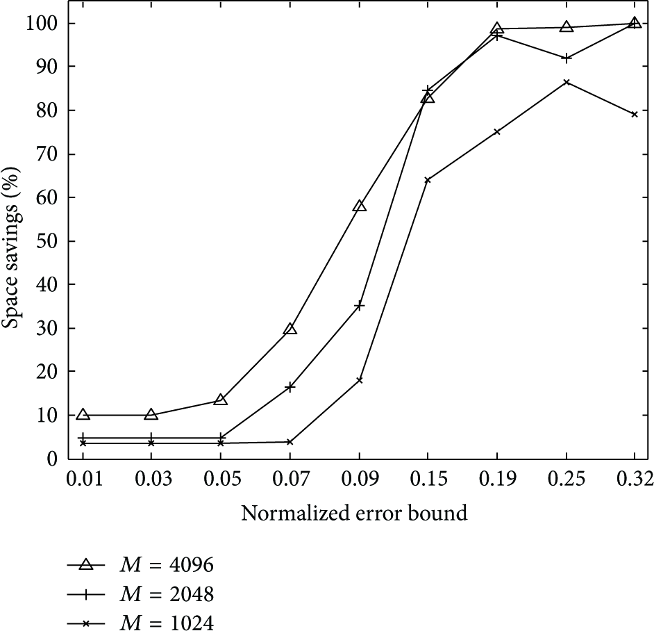
The experimental results have showed that (1) the space savings rate of the AR-MWCEB algorithm is improved with the increase of the normalized error bound. When the normalized error is 0.191, the space savings rate of RACE algorithm is only 87.5% [19]. For the same error bound, the space savings rate of RACE algorithm is always less than that of AR-MWCEB algorithm. (2) To obtain higher space savings rate, PMC-MEAN algorithm [27] should accumulate the processed data in each time as many as possible without exceeding the buffer size of a node. With the number of the samples increasing, multivariate correlation will be weakened so that the absolute error bound increases. However, the AR-MWCEB algorithm determines self-adaptively the number of data involved in the regression by the error bound, and then it can search regression segments in a bigger interval to achieve better compression performance. (3) With respect to the amplitude of attribute no. 3, it has many large high-frequency noises; thus the compression performance is not good for the case of small error bound. (4) When the predefined error bound is small, MWCEB may degenerate into the SWCEB without taking advantage of multivariate correlation, and AR-MWCEB solves this problem.

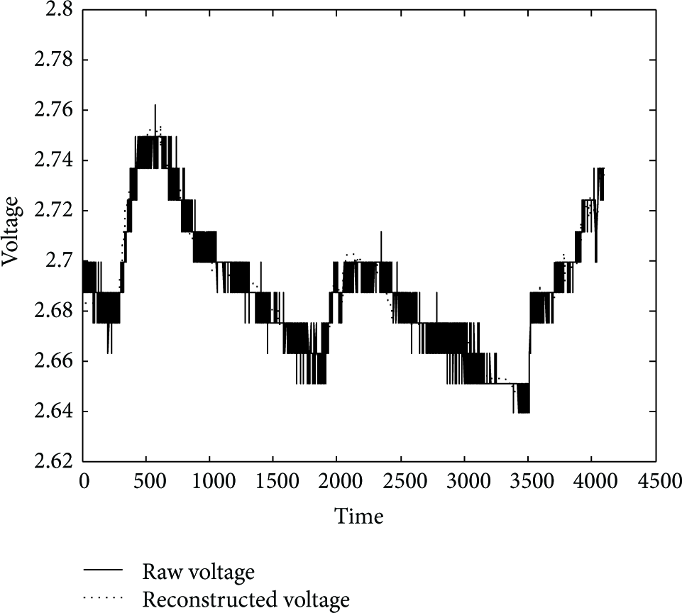
Figure 4 shows the comparison of the reconstructed temperature data with the raw sampling ones, where $M = 2048$ . The AR-MWCEB algorithm has self-adaptively divided these experimental data into 13 segments for regression and the 16 data from the 1521th to the 1536th raw data for direct transmission leading to a space savings rate of 96.9971%. Figure 5 shows the comparison of the reconstructed voltage data with the raw sampling ones, where $M = 4096$ . The AR-MWCEB algorithm has self-adaptively partitioned these experimental data into 10 segments for regression and the 3841th-3856th 16 data for direct transmission resulting in a space savings rate of 98.7549%.

Figure 4

Reconstruction by adaptive regression (no. 0 based on no. 1).

Figure 5

Reconstruction by adaptive regression (no. 3 based on no. 1).

6.2. Nonstationary Multivariate Correlation

When the correlation coefficient matrix varies with time, each attribute may be reallocated into a group and may act as a new role by using the base selection algorithm in terms of new correlation coefficient matrix every once in a while. In literature [21], before sending data each time, the cluster head had to call preprocessing algorithm to analyze and find the attributes with large correlations, so the overhead was large. This problem also occurred in our previous proposed MWCEB algorithm [22]. But the AR-MWCEB algorithm has been greatly improved by using the base selection algorithm to obtain the information about correlations between attributes. It can avoid considering the change of the correlation coefficient matrix and can regroup the attributes in a long time interval. Although the number of the samples involved in regression calculation is automatically determined to ensure that the error is bounded, the time-varying multivariate correlation may lead to worse compression performance. When the data used for the base selection is not the same as the being transmitted ones, the multivariate correlation can be recognized as being nonstationary.

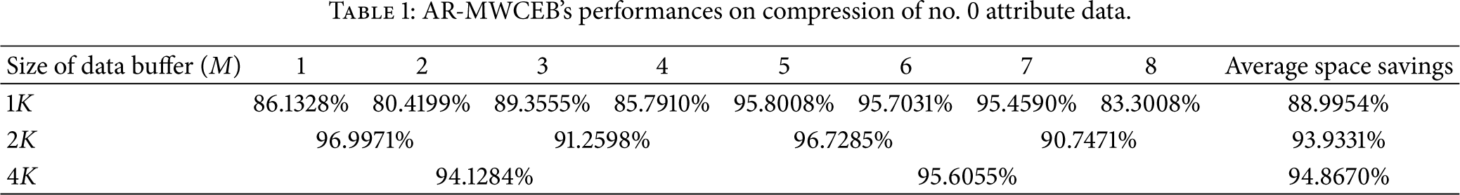
Equally dividing the first 8K times samples of the dataset into 8 segments and calculating the corresponding 8 correlation coefficient matrixes, it is easy to find that these matrices change over time. Next experiments are conducted on transmission of the first 8K times sampling data, where the base selection is based on the beginning 1K sampling data, and attributes no. 0 and no. 3 are determined to take attribute no. 1 as the base signal by the correlation analysis. The attribute correlation is no longer analyzed in a long time. The compression performances of AR-MWCEB algorithm at different time are analyzed when M is 1K, 2K, and 4K, respectively, and are listed in Tables 1 and 2. The used normalized error bound for the temperature (attribute no. 0) is 0.07; the normalized error bound of the voltage (attribute no. 3) is 0.19.

Table 1

AR-MWCEB's performances on compression of no. 0 attribute data.

Size of data buffer (M)	1	2	3	4	5	6	7	8	Average space savings
1K	86.1328%	80.4199%	89.3555%	85.7910%	95.8008%	95.7031%	95.4590%	83.3008%	88.9954%
2K	96.9971%		91.2598%		96.7285%		90.7471%		93.9331%
4K	94.1284%				95.6055%				94.8670%

Table 2

AR-MWCEB's performances on compression of no. 3 attribute data.

Size of data buffer (M)	1	2	3	4	5	6	7	8	Average space savings
1K	75.0488%	49.3652%	71.0938%	87.6953%	96.8262%	96.3867%	84.3262%	83.6426%	80.5481%
2K	97.1680%		82.2510%		99.3164%		93.5791%		93.0786%
4K	98.7549%				98.6084%				98.6817%

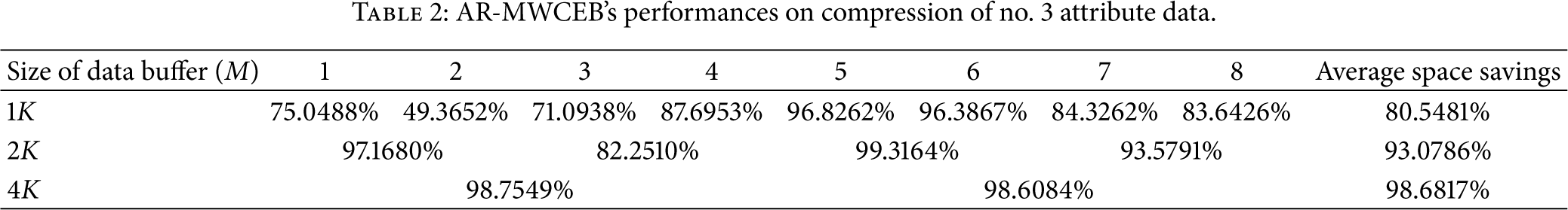
The experiments have shown that (1) since the attribute correlation is reduced with the increase of M, MWCEB algorithm can only divide the sampling data into equal segments, while AR-MWCEB algorithm can self-adaptively segment the data resulting in a smaller error. (2) The attributes are grouped and located roles by the data firstly filling the node buffer. Although the correlation coefficient matrix may change with time, the compression performance of AR-MWCEB algorithm is slightly impacted by the time-varying multivariate correlation. (3) The compression performance is also affected by the distribution of the sampling data. The amplitudes of attribute no. 0 change greatly, and it has few high-frequency noises. For attribute no. 3, its amplitudes change slightly, but it has many large high-frequency noises. Thus, the default error bound for attribute no. 0 is set to a low value, while for attribute no. 3 it is of a larger value.

7. Conclusions

Aiming at effectively compressing the sampling data from the sensor networks node, between which the spatial correlation is nonexistent or nonstationary, this paper proposed a self-adaptive regression-based multivariate data compression scheme with error bound. The algorithms can run independently on each node. Determined by the predefined error bound and compression income, our algorithms can automatically select to transmit the raw data or the regression coefficients and explore the optimal number of the data involved in each regression. The compression performances of the proposed algorithms are also effective when multivariate correlations are reduced or nonstationary. The proposed algorithm is applicable for processing linear multivariate data by researching on using the linear relationship between base and nonbase attributes to represent the compressed results of nonbase attributes.

It is worthy of further research as to how to use a less complicated method to represent the nonlinearity between the base and nonbase attributes. In addition, for the model-based data collection in WSN, how to construct a model with dynamic evolution over time is also going to be our future work.

Footnotes

Acknowledgments

The work in this paper was partly funded by UK EPSRC Project DANCER (EP/K002643/1), EU FP7 Project MONICA (GA-2011-295222), the Science and Technology Planning Project of Hunan Province of China (Grant no. 2011SK3081), the Scientific Research Fund of Hunan Provincial Education Department (Grant no. 12B003), and the National Natural Science Foundation of China (Grant no. 61202439).

References

Kulkarni

R. V.

Förster

Venayagamoorthy

G. K.

Computational intelligence in wireless sensor networks: a survey

IEEE Communications Surveys and Tutorials 2011 13 1 68 96

2-s2.0-79951581342

10.1109/SURV.2011.040310.00002

Zhang

Xie

Yao

Xiao

Guizani

Home M2M networks: architectures, standards, and QoS improvement

IEEE Communications Magazine 2011 49 4 44 52

2-s2.0-79953778099

10.1109/MCOM.2011.5741145

Pottie

G. J.

Kaiser

W. J.

Wireless integrated network sensors

Communications of the ACM 2000 43 5 51 58

2-s2.0-0345851235

Kimura

Latifi

A survey on data compression in wireless sensor networks

Proceedings of the International Conference on Information Technology: Coding and Computing (ITCC ′05)

April 2005

8 13

2-s2.0-24744454159

Wang

C. X.

Yuan

Chen

H. H.

An improved deterministic SoS channel simulator for multiple uncorrelated Ravleigh fading channels

IEEE Transactions on Wireless Communications 2008 7 9 3307 3311

2-s2.0-52349091725

10.1109/TWC.2008.070339

Cheng

Wang

C. X.

Wang

Gao

You

X. H.

Yuan

Huo

Song

Jiao

Cooperative MIMO channel modeling and multi-link spatial correlation properties

IEEE Journal on Selected Areas in Communications 2012 30 2 388 396

Wang

C. X.

Hong

Chen

H. H.

Thompson

On capacity of cognitive radio networks with average interference power constraints

IEEE Transactions on Wireless Communications 2009 8 4 1620 1625

2-s2.0-65949085805

10.1109/TWC.2009.071075

Zarakovitis

Nash bargaining game theoretic scheduling for joint channel and power allocation in cognitive radio system

IEEE Journal on Selected Areas in Communications 2012 30 1 70 81

Bai

Zhang

W. Y.

Xue

G. L.

Tang

Wang

C. G.

DEAR: delay-bounded energy-constrained adaptive routing in wireless sensor networks

Proceedings of the 31st Annual IEEE International Conference on Computer Communications (INFOCOM ′12)

2012

1593 1601

10.

Kabara

Calle

MAC protocols used by wireless sensor networks and a general method of performance evaluation

International Journal of Distributed Sensor Networks 2012 2012 11

834784

11.

Zhang

Energy-efficient cross-layer protocol of channel-aware geographic-informed forwarding in wireless sensor networks

IEEE Transactions on Vehicular Technology 2009 58 6 3041 3052

2-s2.0-67549151164

10.1109/TVT.2008.2010046

12.

Deligiannakis

Kotidis

Roussopoulos

Dissemination of compressed historical information in sensor networks

VLDB Journal 2007 16 4 439 461

2-s2.0-36048989928

10.1007/s00778-005-0173-5

13.

Kanagal

Deshpande

Online filtering, smoothing and probabilistic modeling of streaming data

Proceedings of the IEEE 24th International Conference on Data Engineering (ICDE ′08)

April 2008

1160 1169

2-s2.0-52649107508

10.1109/ICDE.2008.4497525

14.

Kazemeyni

Johnsen

E. B.

Owe

Balasingham

MULE-based wireless sensor networks: probabilistic modeling and quantitative analysis

7321

Proceedings of the 10th International Conference on Integrated Formal Methods

2012

143 157 Lecture Notes in Computer Science

15.

Najafi

Lahouti

Shiva

AR modeling for temporal extension of correlated sensor network data

Proceedings of the International Conference on Software, Telecommunications andComputer Networks (SoftCOM ′06)

October 2006

117 120

2-s2.0-46249121120

10.1109/SOFTCOM.2006.329734

16.

Tulone

Madden

PAQ: time series forecasting for approximate query answering in sensor networks

3868

Proceedings of the 3rd European Workshop for Wireless Sensor Networks (EWSN ′06)

2006

21 37 Lecture Notes in Computer Science

17.

Borgne

Y. L.

Bontempi

Time series prediction for energy-efficient wireless sensors: applications to environmental monitoring and video games

102

Proceedings of the 4th International ICST Conference on Sensor Systems and Software (S-Cube ′12)

2012

Lakshmi Narain College of Technology

63 72

18.

Borgne

Y. L.

Bontempi

Unsupervised and supervised compression with principal component analysis in wireless sensor networks

Proceedings of 1st International Workshop on Knowledge Discovery from Sensor Data (SensorKDD ′07)

2007

55 79

19.

Chen

Mohapatra

RACE: time series compression with rate adaptivity and error bound for sensor networks

Proceedings of the IEEE International Conference on Mobile Ad-Hoc and Sensor Systems

October 2004

124 133

2-s2.0-20344407799

20.

Ciancio

Pattem

Ortega

Krishnamachari

Energy-efficient data representation and routing for wireless sensor networks based on a distributed wavelet compression algorithm

Proceedings of the 5th International Conference on Information Processing in Sensor Networks (IPSN ′06)

April 2006

309 316

2-s2.0-34247335080

10.1145/1127777.1127824

21.

Zhu

T. J.

Lin

Y. P.

Zhou

S. W.

X. L.

Adaptive multiple-modalities data compression algorithm using wavelet for wireless sensor networks

Journal on Communications 2009 30 3 48 53

2-s2.0-64249104342

22.

Zhang

J. M.

Lin

Y. P.

Zhou

S. W.

Ouyang

J. C.

Haar wavelet data compression algorithm with error bound for wireless sensor networks

Journal of Software 2010 21 6 1364 1377

2-s2.0-77954305912

10.3724/SP.J.1001.2010.03518

23.

Song

Wang

C. R.

Gao

DLRDG: distributed linear regression-based hierarchical data gathering framework in wireless sensor network

Neural Computing and Applications 2012 15

10.1007/s00521-012-1248-z.

24.

Sadler

C. M.

Martonosi

Data compression algorithms for energy-constrained devices in delay tolerant networks

Proceedings of the 4th International Conference on Embedded Networked Sensor Systems (SenSys ′06)

November 2006

265 278

2-s2.0-34547441351

10.1145/1182807.1182834

25.

Garofalakis

Gibbons

P. B.

Wavelet synopses with error guarantees

Proceedings of the ACM SIGMOD International Conference on Managment of Data (SIGMOD ′02)

June 2002

476 487

2-s2.0-0036361131

26.

Garofalakis

Kumar

Deterministic wavelet thresholding for maximum-error metrics

Proceedings of the 23rd ACM SIGMOD—SIGACT—SIGART Symposium on Principles of Database Systems (PODS ′04)

June 2004

166 176

2-s2.0-3142770458

27.

Lazaridis

Mehrotra

Capturing sensor-generated time series with quality guarantees

Proceedings of the 19th International Conference on Data Ingineering

March 2003

429 440

2-s2.0-0344496679

10.1109/ICDE.2003.1260811

A Self-Adaptive Regression-Based Multivariate Data Compression Scheme with Error Bound in Wireless Sensor Networks

Abstract

1. Introduction

2. Related Work

3. Preliminaries and Problem Statement

Definition 1 (normalization of the sampling data).

Definition 2 (normalization error).

Definition 3 (∞-norm average error).

Definition 4 (the correlation coefficient matrix).

Definition 5 (the best correlation of attribute X j for the base attributes set).

Definition 6 (the expected income of adding candidate attribute X j to the base attributes set).

4. Base Selection and Coefficient Incremental Calculation for Regression

4.1. Base Selection and Linear Regression

Step 1.

Step 2.

Step 3.

4.2. Incremental Calculation for Regression

Algorithm 1:

Algorithm 2: The AuxCalc function.

Algorithm 3: The IncRegress function.

5. A Self-Adaptive Regression-Based Multivariate Data Compression Algorithm with Error Bound

5.1. The Proposed Algorithm

Algorithm 4: The AR-MWCEB algorithm.

5.2. Properties of the Algorithm

Property 1.

Proof.

Property 2.

Proof.

5.3. Complexity Analysis of the Algorithm

6. Experiments

6.1. Stationary Multivariate Correlation

6.2. Nonstationary Multivariate Correlation

7. Conclusions

Footnotes

Acknowledgments

References

Definition 5 (the best correlation of attribute $X_{j}$ for the base attributes set).

Definition 6 (the expected income of adding candidate attribute $X_{j}$ to the base attributes set).