GPS-Assisted Path Loss Exponent Estimation for Positioning in IEEE 802.11 Networks

Abstract

We present a new adaptive method to calculate the path loss exponent (PLE) for microcell outdoor dynamic environments in the 2.4 GHz Industrial, Scientific, and Medical (ISM) frequency band. The proposed method calculates the PLE during random walks by recording signal strength measurements from Radio Frequency (RF) transceivers and position data with a consumer-grade GPS receiver. The novelty of this work lies in the formulation of signal propagation conditions as a parametric observation model in order to estimate first the PLE and then the distance from the received RF signals using nonlinear least squares. GPS data is used to identify long term fading from the received signal's power and helps to refine the power-distance model. Ray tracing geometries for urban canyon (direct line of sight) and nonurban canyon (obstacles) propagation scenarios are used as the physics of the model (design matrix). Although the method was implemented for a lightweight localization algorithm for the 802.11b/g (Wi-Fi) standard, it can also be applied to other ISM band protocols such as 802.15.4 (Zigbee) and 802.15.1 (Bluetooth).

1. Introduction

The emergence of context-aware computing applications, and location-based services and the proliferation of portable electronic devices have motivated an extensive research on the topic of node or device localization for wireless networks operating under 2.4 GHz ISM band protocols such as Bluetooth, Zigbee, and especially Wi-Fi. Localization is an important issue for the interaction between portable device users and the surrounding networked devices in intelligent environments such as homes, offices, or other intelligent buildings [1, 2].

The localization problem has been a hot research topic in the Wireless Sensor Network (WSN) and Mobile Robotics literature. According to the WSN terminology, a node is a small device with sensing, computing, storage, and communication capabilities, and the node localization problem is defined as “determining an assignment of coordinates for nodes in a wireless ad-hoc or sensor network that is consistent with measured pair wise node distances” [3]. The definition states basically that it is necessary to estimate a distance (range) between the nodes before obtaining coordinates. See [4–6] for more WSN terminology and applications.

A range estimation can be performed using collected measurements from a variety of methods such as acoustic [7–9], directional antenna or antenna array [10, 11], infrared [12], and Received Signal Strength (RSS) measurements [13, 14]. Unlike other ranging methods, RSS-based methods estimate neither distances nor positions from the angle of arrival nor traveling time of the signal. Additionally, no clock synchronization is assumed in the nodes. Only the incoming RF signal is used to infer a range to the transmitter. The basic premise is that the received signal power decay is inversely proportional to the distance. This signal power attenuation is called path loss (PL) and can be quantified by a path loss exponent (PLE). Once the ranges to the landmarks (devices with known positions) are estimated, trilateration methods can be employed to find the location of an unknown position node within a suitable coordinate system.

However, RSS levels are highly unpredictable and the formulation of a path loss model (PLM) as function of distance is a complex issue. This complexity is derived from the fact that the received power level is a combination of different signal propagation mechanisms such as reflection, diffraction, and scattering and absorption losses. Due to these impairments, which depend on the surrounding environment, shadowing and multipath fading are produced. As a consequence estimation errors can be introduced for any RSS-based localization algorithm.

In recent years, RSS-based localization algorithms have been the subject of an increasing interest due to the wide availability of 802.11b/g transceivers and the proliferation of Wireless Local Area Networks (WLANs).

This approach exploits existing WLAN infrastructure and precludes the use of additional hardware such as badges; and wearable sensors, see [15, 16]. In fact, the IEEE 802.11 standard provides the means to obtain the signal strength via the Received Signal Strength Indicator (RSSI). This indicator is defined as “a mechanism by which RF energy is to be measured by the circuitry on a wireless NIC. This numeric value is an integer with an allowable range of 0–255 (a 1-byte value)” [17]. Similar metrics are defined for the IEEE 802.15.4 and IEEE 802.15.1 standards.

The node localization algorithms within previous literature are referred to as GPS-free or GPS-less algorithms. The lack of GPS use can be explained by common drawbacks attributed to several causes such as signal availability, cost, antenna size, and energy consumption. Nowadays, some of these arguments are no longer true. GPS chips can be ubiquitously found in mobile devices such as smart phones, hand helds, and tablets. While GPS chips are available in many devices, there are still many others that do not have it. The existing GPS positioning capability could be used to estimate the PLEs of WLAN access points and the derived PLM employed to enable GPS-free location services.

In this paper we propose a PLE estimation method which uses the RSSI provided by a 802.11b/g transceiver in combination with data collected from a commercial grade GPS receiver. The method builds ray tracing models for typical propagation scenarios such as urban canyon and non-urban canyon cases, and uses them to formulate the design matrix of an observation model. The propagation scenarios take into account the shadowing and multipath effects. The observations are composed of RSSI readings and GPS data. The system of equations of the design matrix is linearized using Taylor series and then solved through least squares. The main contribution of this work is the formulation of a parametric mathematical model which improves the PLE accuracy by using the Equivalent Isotropic Radiated Power (EIRP) and Effective Antenna Aperture (EAA) parameters calculated before obtaining the PLE. A second contribution is the combination of GPS data and RSSI readings in order to identify the RSSI long term behavior.

Depending on the transmitter's power, antenna height, and coverage area, the RF environments where the devices are deployed can be classified as macrocell, microcell, and picocell. In microcell environments the transmitting power of the radios ranges from 0.1 to 1 watt, the RF coverage area ranges from 200 to 1000 m, and the transmitter's height is low (3 to 10 meters) [18]. Environments within buildings are classified as picocells. Indoor-to-outdoor configurations are environments with walls blocking the signal and are characterized by a wall attenuation factor. The algorithm proposed in this work is tailored to microcell RF environments with indoor-to-outdoor coverage configurations; therefore models such as Okumura-Hata, Lee, or Walfisch-Bertoni are not treated here. From this point forward, when we refer to a blind node, we mean a device (smart phone, hand held, tablet, or laptop) whose position needs to be estimated; when we refer to anchor or beacon or landmark nodes, we mean access points (APs) for whose position are already known.

The paper is organized as follows. Section 2 reviews the localization algorithms based on RSSI only and algorithms with RSSI-GPS collaboration. In Section 3 we present the proposed method. Section 4 presents the implantation of the method in real world conditions. In Section 5 the accuracy of the experimental results is discussed, and finally, conclusions and future work are presented in Section 6.

2. Related Work

This section is divided in two parts. The first part reviews papers related to either empirical or theoretical RSSI-based models. In the second part, techniques that rely on both RSSI and GPS to derive power-distance models for node localization are examined. Note there are other methods for RF-based localization such as fingerprinting [19, 20] and Bayesian Networks [21, 22]. These techniques and some others exclude PLE estimation and are not reviewed in this paper.

2.1. PLE from RSSI Measurements

The study of RSSI for different purposes is not a new idea. Some of these purposes are the optimization of the coverage area of wireless networks [23], assessment of links quality for multihop routing protocols [24], and so forth. The use of RSSI as a means for node localization estimation in a WLAN dates back to 2000. For example, [25] proposes the use of an Extended Kalman Filter (EKF) to cope with the noise in the measurements and to maintain a position estimate in harsh conditions. They conducted an empirical experiment to relate signal strength to distance between base and mobile stations. The shortcoming of this work is that it is designed to work within predefined surroundings, in this case an office. The accuracy is one room. In [26] authors propose a lookup-table method for node position triangulation. They also conducted data collection to empirically correlate distance to signal strength. The shortcoming of this works is that it requires an extensive survey at different points in a predefined environment and the consequent table size. In [27] authors proposed an optimal averaging window length of RSSI samples to cope with fading of the power and mobility of the nodes. By modeling the channel's fading with a Rayleigh distribution, they obtained a factor ( $r^2$ ) which multiplies the RSSI samples (w). The authors reported a lower bound mean error of 2.5 m with $w=50$ . The main drawback is that this method is intended for rectangular areas where bacons are placed optimally.

Although these previous works do not calculate a PLE explicitly, they formulate empirical power-distance models based on averaged RSSI measurements surveyed in specific locations. They also address some issues affecting the received power levels such as fading due to multipath, nonline of sight, node mobility, and sampling.

In the following literature review we now focus on localization systems for outdoor environments since PLE estimation was first introduced for such environments. In [28] the authors propose a methodology for PLE estimation in a WiMAX system. Although this methodology is not intended for a WLAN, it is carefully examined in this paper because of the use of common theoretical models to estimate PLE. The first part of the methodology pairs RSSI measurements, expressed in dB units, with distance ( $L[\text{dB}]$ , $d[\text{m}]$ ). In the second part, the authors use the well-known log-distance path loss model to formulate a system of equations. The authors measured propagation losses in two different points with identical conditions (line of sight condition) and formulated a system of two linear equations:

$$\begin{array}{l}{L}_1\left[\text{dB}\right]=a+10*\gamma *{\log }_{10}\left(d_1\right),\\ L_2\left[\text{dB}\right]=a+10*\gamma *{\log }_{10}\left(d_2\right),\end{array}$$

(1)

where a is a coefficient that accounts for frequency and other propagation factors, γ is the PLE, and d is distance in meters between the transmitter and the receiver. Solving the system and using several measurements the authors obtained the following empirical path loss model $L[\text{dB}]=123.02+10*2.687*{\log }_{10}(d)$ .

In [29] the authors used the Okumura-Hata model to calculate two different PLEs in a WiMAX network, although the Okamura-Hata model is usually applied in macrocell environments (distances greater than 1 km). They formulated two different map-supported PLMs from RSSI observations. One PLM corresponds to an “urban canyon” area while the other for “non-urban canyon.” The developed models considered the type of area based on city map and road network information.

Note that an urban canyon area is an area where there exists an open street between the receiver and the transmitter. Therefore, the signal reaches longer distances than in areas with obstacles. On the other hand, an area with considerable obstacles is classified as noncanyon.

Next, we shall review works which estimate PLE for WLAN in indoor environments. Authors in [30] proposed and implemented a system framework which consists of a central server, a base station, and four beacon nodes. The algorithm dynamically estimates a PLE between the beacons and the blind node. The base station receives the RSS values collected by the beacons nodes and sends them to the server. The authors also employed the log-distance path loss formula, but they add a stochastic component:

$$\begin{array}{cc}& \text{PL}\left(d\right)=\text{PL}\left(d_0\right)-10\alpha {\log }_{10}\left(\frac{d}{d_0}\right)+X_{\sigma },\end{array}$$

(2)

where $\text{PL}(d)$ denotes the path loss in dB as function of distance d, in meters, away from sender; $\text{PL}(d_0)$ is a path loss constant at a reference distance $d_0$ ; α is the PLE; and $X_{\sigma }$ is Gaussian noise in dBm units. The $X_{\sigma }$ values account for the long term variability. The α exponent is estimated using the following formula:

$$\begin{array}{cc}& \alpha =\frac{-{\sum }_{i=1}^n\left(\text{PL}\left(d_i\right)-\text{PL}\left(d_0\right)\right)}{{\sum }_{i=1}^{n}10\left(\log d_i\right)},\end{array}$$

(3)

where n is the number of RSSI measurements at distances $d_i$ . Basically, (3) expresses α in terms of an averaged ratio between path loss and the logarithm of distance using all measurements recorded. This averaged PLE is used to obtain distances between the blind node and the four beacons. Finally, a polygon method was used to obtain the blind node's coordinates.

Model (2) is commonly used in macrocell scenarios by setting the $d_0$ reference distance to 1 km. Although the formula was modified for microcell scenarios (setting $d_0$ to 1 and 100 meters), we do not think that this is the most suitable PLM because of the particularities of such environments.

2.2. RSSI Measurements and GPS Data

Some of the first applications of collaborative GPS/Wi-Fi were geocaching, wardriving, and the elaboration of signal coverage maps. Geocaching is a recreational outdoor activity in which the users seek containers with the aid of GPS receiver and mobile devices. War driving is the activity of searching Wi-Fi wireless networks in a moving vehicle, using a portable computer or other devices connected to a GPS. A signal coverage map is a map with geographic information of areas where a wireless networks are deployed. It represents signal intensity areas (strong or weak) with contour lines or colors.

In [31] the authors presented a solution for manual deployed networks called Walking GPS. It works by attaching a GPS receiver to a node called GPS mote. This node first converts its latitude and longitude coordinates into a local coordinates system and then it broadcasts its position to the rest of the nodes. When the carrier (person or vehicle) places a new node in a certain position and turns it on, the node immediately receives the broadcast packet from the GPS mote and estimates its own position. On the other hand, if a node is turning on after being deployed, it needs to ask its neighbors for their positions in order to trilaterate its own position. The main drawback of this solution is that it was tested in an ideal propagation scenario (open field environment). Moreover, the blind nodes were deployed within a predefined grid.

In [32] the authors proposed a multisensor fusion solution with data from three sources: a GPS, a radio propagation map, and a WLAN positioning system. They divided the radio map into three areas: indoor, outdoor, and shaded (a shaded area is an area surrounded by buildings or in closed places). The areas are covered by three fixed APs. The algorithm consists of two phases: offline and online. In the offline phase they collect RSSI measurements at predefined locations in the map. At these locations, they estimate the expected RSSI values using an equation similar to (3) with a reference distance of 1 meter. Calculating the ratio between the observed and the expected RSSI, they model the corresponding multipath. Based on these ratios, a polynomial fit function is computed for all the predefined locations. Using this information and trilateration, the WLAN positioning system estimates a blind node preliminary position. Finally, in the online phase the GPS is used to identify the area (indoor, outdoor, or shaded) to improve the estimated positions.

In [33] the authors presented an outdoor WiFi localization system assisted by GPS. The system uses a unidirectional Yagi type antenna to triangulate the location of APs using the angle of arrival of the received signal. The angle of the received signal is measured with a GPS compass which is rotated with the antenna and the WiFi receiver at the same time. All the equipment was mounted on a motorized rotating base. The proposed algorithm consists of the following steps: (i) place the equipment at two different measurements points $M_1(x_1,y_1)$ and $M_2(x_2,y_2)$ ; (ii) find the respective ${\theta }_1$ and ${\theta }_2$ which corresponds to the angles at which the maximum RSSI are observed; (iii) find the slopes $m_1=\tan {\theta }_1$ , and $m_2=\tan {\theta }_2$ and calculate $c_1$ and $c_2$ using the line equation $y=mx+c$ ; and (iv) find the intersection point for $y_1=m_1{x}_2+c_1$ and $y_2=m_2{x}_2+c_2$ . This intersection point corresponds to the estimated location of the AP.

3. Proposed Solution

The models described in Section 2 express a power distance relationship based on the attenuation of the signal's power as it propagates. Such attenuation roughly obeys the inverse power law:

$$\begin{array}{cc}& P_r=\mathrm{\hspace{0.17em}\hspace{0.17em}}\frac{1}{d^{\alpha }},\end{array}$$

(4)

where $P_r$ is the power received in watts, α is the PLE (equal to 2 in free space conditions), and d is the distance between the transmitter and the receiver in meters. However, the receiver power attenuates at a much higher rate and exponent $\alpha >2$ . A higher α can be explained in terms of losses caused by propagation mechanisms, such as diffraction, scattering, reflection, and refraction. For a detailed explanation refer to [34]. The combination of these mechanisms is responsible for power variations in the RSSI readings. These variations are commonly classified as slow variation or long term fading and fast variations or short term fading. Fast variations are characterized by rapid fluctuations in the RSSI levels over very short distances. On the other hand, long term fading, also called large scale path loss, is due the increasing distance as the receiver moves away from the transmitter.

A suitable mathematical tool to model these propagation mechanisms and their effects on RSSI variability is ray-tracing. An electromagnetic wave (EM) is composed of electric (E) and magnetic (B) fields. These fields are perpendicular to each other and the direction of the wave is obtained from the cross product of $\mathbf{E}\times \mathbf{B}$ . The result is the Poynting vector (S) that can be modeled as a ray. In ray tracing, a ray is an imaginary straight line depicting the path light travels. Using geometrically defined propagation scenarios, the trajectory of different S rays can be computed.

The proposed method is divided into three phases. In the first phase the EIRP and PLE parameters are estimated using the observation model. In the second phase, PLMs for each landmark are formulated in order to translate RSSI measurements into ranges. In the final phase, these ranges are used to estimate the locations of one or more blind nodes. Next, each phase is described in detail.

3.1. Observation Model Formulation

The formulation of the system to infer the EIRP and PLE is expressed as follows:

$$\begin{array}{cc}& \mathbf{z}=H\left(\mathbf{x}\right)\beta +\mathbf{v},\end{array}$$

(5)

where $\mathbf{z}=[z_1{z}_2{z}_3\cdots z_n]$ is a $1\times n$ vector of RSSI observations recorded in dB units at different distances ranging from 1 to 200 meters. Each $z_i$ represents the measurements at a particular distance (see Section 4); $H(\mathit{x})$ is the design matrix representing the ray tracing models; $\beta =[{\theta }_1,{\theta }_2]$ is the vector of parameters to be estimated; and lastly v is a Rayleigh distributed random variable which accounts for fast variation in short distances [35]. The block diagram for this phase is shown in Figure 1.

Figure 1

Schematic diagram for phase 1.

Mathematical models expressed in matrix H relate the observations z with the parameter vector β. These models are ray tracing equations for an urban canyon and a non urban canyon. Matlab scripts provided by [36] are used to construct the geometry for the two scenarios. See Figure 2.

Figure 2

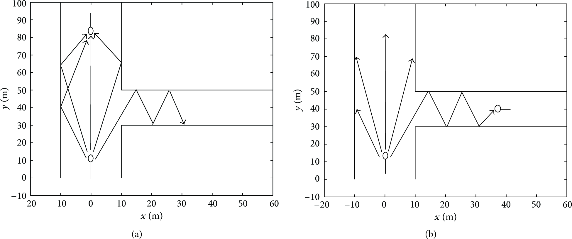
Ray tracing representation of signals traveling distances in (a) urban canyon propagation scenario and (b) nonurban Canyon propagation scenario.

The models perform the addition of direct and reflected rays and calculate the resulting received power at different points in the scenarios. This is done by calculating the average of vector S trough an area, that is, the power flux density (PFD). First average S is expressed in terms of E-field strength and then it is related to the Effective Antenna Aperture (EAA) area of the receiving antenna as follows:

$$\begin{array}{cc}& P_r={\varnothing A}_r.\end{array}$$

(6)

The PFD represents the field strength at the receiver's antenna (in W/m² units) and it is defined as

$$\begin{array}{cc}& \varnothing =\frac{1}{2}\frac{{\left|e\right|}^2}{120\pi },\end{array}$$

(7)

where $|e|$ is the magnitude of the electric field radiated in the far-field region by the source point. 120π is the impedance of free space (in Ohms). EAA is defined as

$$\begin{array}{cc}& A_r=\frac{{\lambda }^2·g_r}{4\pi ·l_r},\end{array}$$

(8)

where $g_r$ is the receiving antenna gain in dBi, and $l_{\text{r}}$ is the system loss at the receiver. PFD is defined as follows:

Expressing (6) as a function of distance

$$\begin{array}{cc}& {\mathrm{\hspace{0.17em}\hspace{0.17em}}P}_r\left(d_0\right)=A_r\frac{{\left|e_T\left(d_0\right)\right|}^2}{2\eta },\end{array}$$

(9)

where $e_T$ is the modulus of complex number $e_T$ and represents the total field strength of the rays combining at the receiver ( $e_T=e_0+e_1+e_2+e_3$ ). The term $e_0$ represents the direct ray field strength; $e_1$ represents the ray reflected in the ground; and $e_2$ , $e_3$ represent the rays reflected on walls. The formulas for each term are

$$\begin{array}{l}{e}_0=\sqrt{\frac{60pg}{l}}\left\{\frac{e^{\left(-jk{d}_0\right)}}{d_0}\right\},\\ e_1=\sqrt{\frac{60pg}{l}}\left\{\text{GR}\frac{e^{-jk\left(d_0+d_1\right)}}{d_0+d_1}\right\},\\ e_2=\sqrt{\frac{60pg}{l}}\left\{\text{WR}\frac{e^{-jk\left(d_0+d_2\right)}}{d_0+d_2}\right\},\\ e_3=\sqrt{\frac{60pg}{l}}\left\{\text{WR}\frac{e^{-jk\left(d_0+d_3\right)}}{d_0+d_3}\right\},\end{array}$$

(10)

where $d_0$ is the direct ray distance between the transmitter and the receiver, $d_1$ is the additional distance the ray travels due to reflection on the ground, $d_2$ and $d_3$ are the additional distances due to wall reflections. These additional distances ( $d_1$ , $d_2$ , $d_3$ ) are fixed according to the specified geometry. Constants WG and WR are ground and wall reflections coefficients, respectively. Substituting (10) in (9) we obtain:

$$\begin{array}{l}{A}_r|\sqrt{\frac{60pg}{l}}(\{\frac{e^{\left(-jk{d}_0\right)}}{d_0}+\text{GR}\frac{e^{-jk\left(d_0+d_1\right)}}{d_0+d_1}\\ {\hspace{1em}\hspace{1em}\phantom{+\sqrt{\frac{60pg}{l}}}+\text{WR}\frac{e^{-jk\left(d_0+d_2\right)}}{d_0+d_2}+WR\frac{e^{-jk\left(d_0+d_3\right)}}{d_0+d_3}\})|}^2{\left(2\eta \right)}^{-1}.\end{array}$$

(11)

The term $p_t{g}_t/l_t$ is the EIRP and one of the parameters to estimate. Substituting (11) in matrix $H_A$ in (5), the resulting system is

$$\begin{array}{cc}& \mathbf{z}=\left[\begin{array}{c}{Pr}_1\left(d\right)\\ ⋮\\ {Pr}_n\left(d\right)\end{array}\right]\mathrm{\hspace{0.17em}\hspace{0.17em}}\beta +\mathbf{v}\mathbf{.}\end{array}$$

(12)

3.2. Range Estimation

After linearizing (12) using Taylor series, we apply least squares to estimate EIRP and EAA. In order to obtain a more accurate PLE, we use transmitted power, $p_t$ received power, $p_r$ transmitter antenna gain, $g_t$ receiver antenna gain, $g_r$ , transmitter system loss, $l_t$ and receiver system loss, $l_r$ , to formulate a new system:

$$\begin{array}{cc}& \mathit{z}=\left[\begin{array}{c}{Pr}_1\left(d\right)\\ ⋮\\ {Pr}_n\left(d\right)\end{array}\right]\mathrm{\hspace{0.17em}\hspace{0.17em}}\beta +\mathit{n}.\end{array}$$

(13)

In this formulation, the RSSI observation vector z contains the short term or slow variations which were filtered out of the raw readings. This extraction was carried out by a running mean. A running mean calculates the signal strength averages within a certain length distance interval. Commonly used length interval ranges from 20 to 40 times λ [37]. These averages are indexed and the vector z is formed where $n=1\cdots \max$ _distance. The variable $\mathit{n}$ is a normal distributed random variable which accounts for slow variations in long term fading. The model for this system's design matrix is the logarithm of the Friis formula:

$$\begin{array}{l}{\mathrm{\hspace{0.17em}\hspace{0.17em}}p}_r\left(d\right)=\left(p_t+g_t+g_r-l_t-l_r\right)+\left(10·2·{\log }_{10}\left(\frac{\lambda }{4\pi }\right)\right)\\ +\gamma ·10·{\log }_{10}\left(d\right).\end{array}$$

(14)

The terms between parentheses are constant and were calculated in the previous step; therefore the parameter, $\beta =[\theta ]$ , to be estimated is the PLE, γ, and remains in the last term.

Seven APs located in the University of Calgary campus were selected as landmarks during the data collection process (Refer to Section 5 for more information) having the following service set identification (ssid): ENA_131, ENE_136 and NM_110, KNB_125u, KNB_132, MC_184, and MC_197. After the method was applied to the signal strength received from them and to the GPS data collected, a PLE and a path loss model for each one were estimated. Table 1 lists ssid, estimated PLE values, and the actual UTM coordinates for the landmarks. In this work the UTM system is employed due to its use of meters instead of degrees of latitude and longitude.

Table 1

AP ssid	Actual coordinates	Estimated PLE ( γ )
ENA_131	N: 5662636.17 E: 700932.53	2.42
ENE_136	N: 5662669.42 E: 700841.48	2.35
NM_110	N: 5662542.19 E: 700931.53	2.31
KNB_125u	N: 5662445.24 E: 700805.63	2.40
KNB_132	N: 5662421.01 E: 700798.60	2.41
MC_184	N: 5662452.13 E: 700879.63	2.52
MC_197	N: 5662474.47 E: 700927.79	2.55

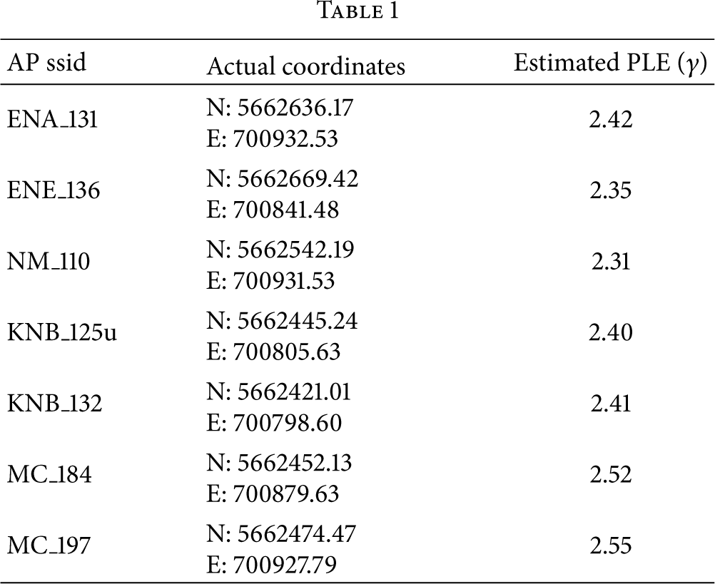
Figure 3 shows short term received power and the corresponding long term path loss model for APs: ENA_131, ENE_136, and NM_110. Figures 3(c) and 3(d) correspond to non-urban canyon and reflect more harsh propagation conditions.

Figure 3

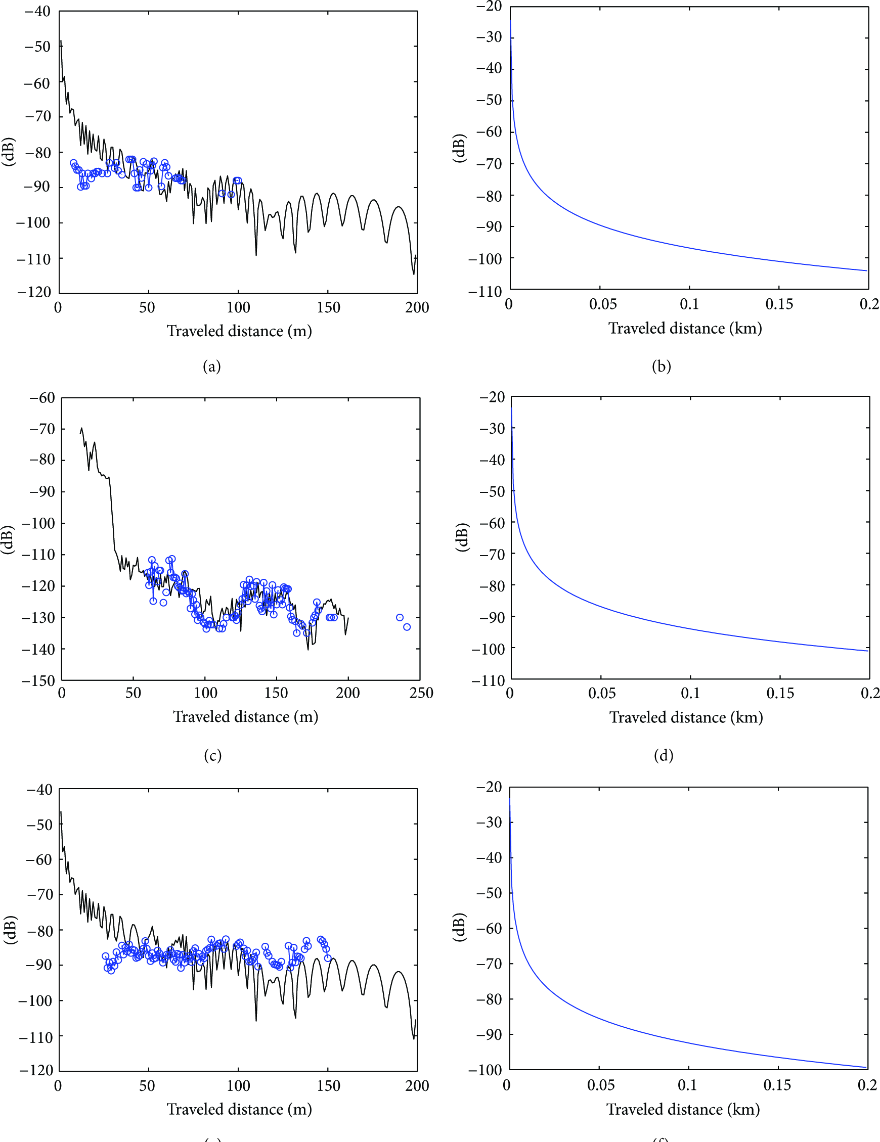
(a) AP ENA_131 short term received signal power for an urban canyon model. (b) Corresponding long term distance model with $\text{PLE}=\mathrm{2.42}$ . (c) AP ENE_136 short term received signal power for non-urban canyon. (d) Corresponding long term distance model with $\text{PLE}=2.35$ . (e) AP NM_110 short term received signal power for urban canyon model. (f) Corresponding long term model with $\text{PLE}=2.31$ .

3.3. Node Localization

In order to determine the blind node position in 2D space, n landmarks are employed. Although two landmarks would be enough, there would be two possible solutions. A third landmark reduces the estimation to a unique solution. With the ranges estimated from a blind node to n landmark APs and the coordinates of the latter, the method can formulate the following system of nonlinear simultaneous equations:

$$\begin{array}{l}{\rho }_1=\mathrm{\hspace{0.17em}\hspace{0.17em}}\sqrt{{\left(x_1-x_u\right)}^2+{\left(y_1-y_u\right)}^2+{\left(z_1-z_u\right)}^2},\\ {\rho }_2=\mathrm{\hspace{0.17em}\hspace{0.17em}}\sqrt{{\left(x_2-x_u\right)}^2+{\left(y_2-y_u\right)}^2+{\left(z_2-z_u\right)}^2},\\ \hspace{1em}⋮\\ {\rho }_n=\mathrm{\hspace{0.17em}\hspace{0.17em}}\sqrt{{\left(x_n-x_u\right)}^2+{\left(y_n-y_u\right)}^2+{\left(z_n-z_u\right)}^2},\end{array}$$

(15)

where ( $x_1,y_1$ ), ( $x_2,y_2$ ), and ( $x_3,y_3$ ) are the APs known coordinates; ( $x_u,y_u$ ) is the position to find; and ${\rho }_1,{\rho }_2,\dots ,{\rho }_n$ are the estimated ranges. UTM Northing and Easting coordinates are identified with y and x, respectively. Because the blind node and the APs are placed at ground level, the z coordinate is constant with an altitude of 1112.4 meters. Because the number of equations is larger than the number of unknowns the system has no analytical solution. However, it can be solved through linearization and iteration. First we decompose the unknowns into approximate and incremental components: $x_u={\widehat{x}}_u+\mathrm{\Delta }{x}_u$ , $y_u={\widehat{y}}_u+\mathrm{\Delta }{y}_u,z_u={\widehat{z}}_u+\mathrm{\Delta }{z}_u$ , where $\mathrm{\Delta }{x}_u$ , $\mathrm{\Delta }{y}_u$ , $\mathrm{\Delta }{z}_u$ are the unknowns, and ${\widehat{x}}_u$ , ${\widehat{y}}_u$ , ${\widehat{z}}_u$ are considered known by assigning them an initial value. By substituting these values in (15) and differentiationing we obtain:

$$\begin{array}{l}p\left({\widehat{x}}_u+\mathrm{\Delta }{x}_u,{\widehat{y}}_u+\mathrm{\Delta }{y}_u,{\widehat{z}}_u+\mathrm{\Delta }{z}_u\right)\\ \hspace{1em}=p\left({\widehat{x}}_u,{\widehat{y}}_u,{\widehat{z}}_u\right)+\frac{\partial p\left({\widehat{x}}_u,{\widehat{y}}_u,{\widehat{z}}_u\right)}{\partial {\widehat{x}}_u}\mathrm{\Delta }{x}_u\\ \hspace{1em}\hspace{1em}+\frac{\partial p\left({\widehat{x}}_u,{\widehat{y}}_u,{\widehat{z}}_u\right)}{\partial {\widehat{y}}_u}\mathrm{\Delta }{y}_u+\frac{\partial p\left({\widehat{x}}_u,{\widehat{y}}_u,{\widehat{z}}_u\right)}{\partial {\widehat{x}}_u}\mathrm{\Delta }{z}_u+\cdots .\end{array}$$

(16)

The series is truncated after the first-order partial derivatives eliminating nonlinear terms. With initial values for ${\widehat{x}}_u$ , ${\widehat{y}}_u$ , ${\widehat{z}}_u$ , new values for $\mathrm{\Delta }{x}_u$ , $\mathrm{\Delta }{y}_u$ , $\mathrm{\Delta }{z}_u$ can be calculated and used to modify original ${\widehat{x}}_u$ , ${\widehat{y}}_u$ , ${\widehat{z}}_u$ values. The modified values are used again to find new deltas. This iteration continues until the absolute values of deltas are within a certain predetermined limit. For a detailed explanation of this process see [38].

For instance, with Wi-Fi only data collected at test point 5662622.36N, 700894.86E, and the PLEs and coordinates of APs ENA_131, ENE_136, and NM_110 (listed in Table 1), the following mean ranges were obtained: ${\rho }_1=43.9158$ meters, ${\rho }_2=60.5400$ meters, and ${\rho }_3=65.5568$ meters. Real ranges are: 38.58, 68.42, and 91.43 meters. After solving the system, the resulting estimated coordinates for the blind node were: $x_u=5662600$ , $y_u=700900$ , and $z_u=1112.4$ (red color balloon in Figure 4). In this particular case the position error was 22.9432 m.

Figure 4

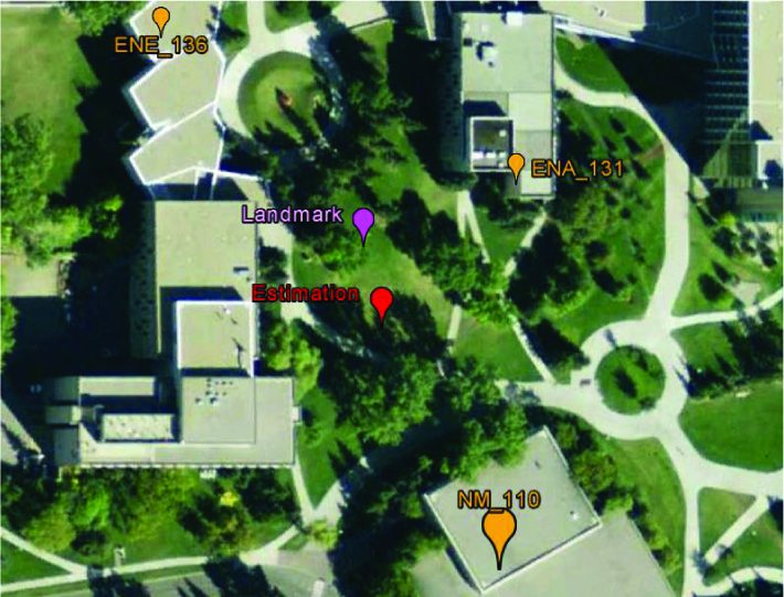
One example result and visualization on Google Earth.

4. Implementation of the Method

In order to test our proposal, several experiments were performed at a university campus. The data collection process consists in recording the signal strength from nearby Wi-Fi APs. The geographic location of the points where data was collected was also logged and paired with the Wi-Fi data at rate of 3 Hz. The data collection was carried out with a laptop and a GPS Garmin model GPSmap 60CSx. In the laptop the inSSIDer program was installed and the GPS receiver was connected via USB port. The campus infrastructure consists of 1280 APs with transmission rate of 54 Mbps, maximum Tx sensitivity of +17.0 dBm, and minimum Rx sensitivity of −73.0 dBm. 87 out of 1280 APs were identified along with their geographic positions, but only seven were used in the experiments (see Table 1). The data was collected during several random walks each 15 minutes long and was carried out on August 7, 11, 15, and 29 and June 15 and 23, 2011. All tests took place within the area located between the three buildings. See Figure 4. The data was logged in the GPS eXchange format:

•  

<time>2011-08-16T00 : 26 : 46.0Z</time>

 

<wpt lat=“51.079936” lon=“−114.133793”>

 

<MAC>00 : 0B : 86 : D6 : CB : 43</MAC>

 

<RSSI>−78</RSSI>

The <time> tag stores the UTC time when the measurement was taken. The <wpt> tag stores the latitude and longitude where the measurement was taken. The <MAC> tag stores the physical address of the AP that sent the signal. The tag <RSSI> stores the power level of that signal. To obtain the distance between the point where the data was collected and the point where the transmitting AP is located, we use the Spherical Law of Cosines. This law gives accurate results down to distances as small as 1 meter. Finally, the data was classified according to the MAC address of the identified APs and sorted from closest to farthest distance in order to obtain the observations vector $\mathbf{z}=[z_1{z}_2{z}_3\cdots z_n]$ .

5. Experimental Results

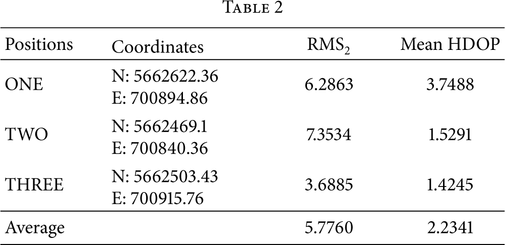
After data collection and model formulation phases, three blind node positions within the campus were selected to test our method. The coordinates of these positions are listed in the second column of Table 2. In order to evaluate accuracy of the results, Wi-Fi only readings and GPS only waypoints were collected at these positions. Note that this number of positions represents the best readings for both Wi-Fi and GPS signals in our experimental scenario. The overall PLE estimation can be improved as the number of blind node position readings is increased. However, this is subject to good quality readings.

Table 2

Positions	Coordinates	RMS2	Mean HDOP
ONE	N: 5662622.36 E: 700894.86	6.2863	3.7488
TWO	N: 5662469.1 E: 700840.36	7.3534	1.5291
THREE	N: 5662503.43 E: 700915.76	3.6885	1.4245
Average		5.7760	2.2341

Before evaluating results, it is necessary to select the appropriate accuracy metrics. Since this work uses a GPS receiver to infer a power-distance model, it is necessary to employ common metrics used by GPS manufacturers such as Circular Error Probable (CEP), one-dimensional root mean square ( ${\text{rms}}_1$ ), and two-dimensional root mean square ( ${\text{rms}}_2$ ). See [39] for the definitions of these and other metrics.

Since the proposed localization algorithm is intended for portable electronic devices such as tablets, laptops, or handhelds, the localization takes place in a 2D map. Therefore, horizontal accuracy metric ${\text{rms}}_2$ is selected. The metric ${\text{rms}}_2$ is the square root of the average of the squared horizontal error and is calculated as follows:

$$\begin{array}{cc}& {\text{rms}}_2=\mathrm{\hspace{0.17em}\hspace{0.17em}}\sqrt{{\sigma }_x^2+{\sigma }_y^2},\end{array}$$

(17)

where ${\sigma }_x^2$ and ${\sigma }_y^2$ are the root mean square errors of the x and y components of the estimated positions, if measurements and model errors are assumed uncorrelated and the same for all observations. If this assumption is not fulfilled, the ${\sigma }_x^2$ and ${\sigma }_y^2$ are the variance of the x and y components. A related metric is Horizontal Dilution of Precision (HDOP). It is defined as the ratio of ${\text{rms}}_2$ to the root mean square of the range errors. The closer the HDOP value is to 1 the higher the accuracy obtained. These two metrics are employed to quantify errors within this section.

5.1. GPS Only Data

7963 GPS waypoints were collected at positions ONE, 6792 at positions TWO, and lastly 8340 at position THREE. These waypoints were processed in order to extract Northing and Easting coordinates and HDOP. With this information the horizontal error position with respect to the actual coordinates of position ONE, TWO and THREE was calculated. The results for metrics ${\text{rms}}_2$ and HDOP are shown in Table 2.

5.2. Wi-Fi Only Measurements

Now, the same metrics are calculated for the WiFi only readings. In this case 5116 readings were collected at the test positions. Three landmark APs were selected for positions ONE and TWO, and only two for position THREE. Using the PLEs obtained in Section 4 for each AP, ranges to them were estimated. With the APs actual coordinates, the real ranges were calculated (listed in Table 3). Using this information, the method derived estimated positions for the three test points. The resulting rms₂ and HDOP are summarized in Table 3.

Table 3

	Estimated mean ranges to APs (meters)	Real ranges to APSs (meters)	RMS2	Mean HDOP
Position ONE	ENA_131: 43.9158 ENE_136: 60.5400 NM_110: 65.5568	38.58 68.41 91.43	15.7322	0.7866
Position TWO	KNB_125u: 48.6630 KNB_132: 51.5463 MC_184: 41.9375	51.74 75.70 41.32	32.2975	1.7112
Position THREE	MC_197: 23.2717 NM_110: 34.2559	30.09 43.91	6.0423	0.5857
Average			18.024	1.0278

Comparing Tables 2 and 3, it can be seen that the ${\text{rms}}_2$ measure of our results is almost 3 times the GPS ${\text{rms}}_2$ measure. It should be noted that a comparison of GPS and WiFi derived HDOP values is not appropriate as each method has its own unrelated ranging error.

6. Conclusions and Future Work

In this paper an adaptive method to formulate a power-distance model and infer distances to AP landmarks was proposed. The method is formulated as state space system. The method uses GPS and RSSI data to identify the short term and long term behavior on of the received signal power. The system's design matrix includes the ray tracing models (canyon and non-canyon) needed to estimate the PLE. Based on this the distance to each RSSI measurement source is estimated and consequently its respective position. Once the GPS-Assisted PLE model is derived at any time a user without GPS (for instance, equipped with a WiFi-only device) is capable of estimating her/his position.

A case study was implemented employing an 802.11 based network and data from a consumer-grade GPS receiver. The results were encouraging. The ${\text{rms}}_2$ error using only RSSI and the derived GPS-Assisted PLE model was, on average, 18.02 meters. On the other hand, the average error using only a consumer grade GPS was 5.77 meters. This means that the proposed method is capable of formulating propagation models that overcome signal impairments and deliver results which are approximately 3 times the GPS error. The proposal results are promising and its accuracy is higher than disable GPS Selective Availability service which consisted of 100 m horizontal.

Although there are different works in the literature review that combine GPS and RSSI, none of them explicitly produce a PLE model. However, there are related works with real implementations which obtain a higher accuracy but they require additional GPS hardware or manual deployments in predefined grids.

Future work includes additional case studies for protocols such as 802.15.4 and 802.15.1. Also, since least squares are the basis of the proposed methodology this can be extended to other applications such as blind node tracking based on Kalman Filters.