Sage Journals: Discover world-class research

Abstract

The steering stability of vehicle was the most important part of vehicle handling and stability. The stability analysis of vehicle negotiating a curve in the plane was studied through simulation. The vehicle dynamics model used in this paper had two degrees of freedom with nonlinear tire characteristics. When two vehicle state variables, namely, velocity and steering angle, were changed, the GA and phase space analysis were used to compute the equilibrium points and analyze the phase space characteristics of vehicle system. Considering the nonlinear tire characteristic, the working region of tire was figured out and compared, while the vehicle was under different operating conditions. From the analysis results, it could be concluded that working in the nonlinear region of tire characteristic was the ultimate reason of vehicle instability. The knowledge derived from simulation results could dramatically enhance the understanding of stability of the actual vehicle negotiating a curve on an even surface. Such knowledge was a prerequisite for robustly designing the chassis, such as steer-by-wire, which would be the topics of future work.

1. Introduction

The steering stability of vehicle was important for both vehicle performance and safety. The nonlinear tire behavior played a critical role in vehicle dynamics. The vehicle performance in the linear range of tire response, typically within the range 0.3~0.4 g of lateral acceleration, had been extensively researched and was well understood [1]. However, beyond this range, the response of tire characteristic was nonlinear and tire forces saturation would lead to a relative degradation in the performance capability. In the nonlinear range of tire characteristic, vehicle handling behavior was not well understood. Especially, as the driving conditions changed from moderate cornering on a dry road to hard cornering on a low-friction road, vehicle might display unstable dynamics characteristics. In worse case, the vehicle would fall into a spin [2].

In the area of controlling vehicle handling dynamics, a great deal of researches had been conducted, such as literatures [3, 4]. It was well known that to control a nonlinear system a deep insight into the dynamics was required and this was particularly true if limit cycles and bifurcations existed [5]. A nonlinear system generally had more than one single equilibrium point. The local linear model was sufficient to capture the behaviors of vehicle in the neighborhood of equilibrium point, but should not be used to represent the system if the distance between different equilibrium points was large. The stability analysis of vehicle system presented in the literature [3, 4] was built upon the assumption of linear tire force characteristics even though the linear relationship applied only locally. To date, Inagaki et al. [6] proposed a phase portrait method, which described side slip angle and yaw rate in a planar diagram to analyze the stability of vehicle system considering the nonlinear tire characteristics. With Inagaki's phase portrait method, Ono et al. [7] suggested that a saddle-node bifurcation occurred when the side slip angle of tire increased up to a level and the vehicle would be out of control thereafter. Below this level, the vehicle system had one stable and two unstable equilibrium points. Catino et al. [8] achieved some similar results using a software package called MATCONT. Phase portrait method used by Inagaki and Ono was, to some extent, convenient and helpful for analyzing the global feature of vehicle system, but it made the investigation of bifurcations characteristics of vehicle system difficult. An analytical method was developed to examine and predict the dynamics behavior of vehicle motion by Lukowski [9]. Dai and Han [10] discovered a Hopf bifurcation using this method. However, this analytical method was complex from the point of design of control module of vehicle system. In this paper, the phase plane was used to analyze the stability region of vehicle during different steering conditions and the GA method was first employed to solve out the bifurcation points of vehicle system under different conditions. To further analyze the instability mechanism of vehicle system, the working regions of tire were figured out and compared under different operating conditions. Those contents made a primary contribution to the understanding of the loss of stabilization of vehicle.

In order to enhance the understanding of vehicle planar motion stability and improve traffic safety, this paper was organized as follows. First, we presented a simplified vehicle model for stability analysis with two degrees of freedom and nonlinear tire characteristic. Second, a method of computing the equilibrium points of vehicle system was proposed based on the GA. Third, when two independent input parameters referring to running conditions, namely, steering angle and velocity, were varied, the GA and phase space analysis were used to compute the equilibrium points and analyze the phase space characteristics of vehicle system negotiating in low-friction road. Forth, considering the nonlinear tire characteristic, the working regions of tire were figured out and compared, while the vehicle was driving under different operating conditions. Finally, the concluding remarks and implications of the work were collected together and presented.

2. Vehicle Model

There were two typical vehicle models considering the degrees of freedom and linearity of vehicle system. A simplified vehicle model was useful for analyzing the vehicle's moving characteristic and dynamic feature in a simple way, while a complex model (such as a multibody dynamic model in MSC.ADAMS) was appropriate for carrying out the accurate simulation analysis [11]. In this paper, the mechanical model used for the stability analysis of vehicle system negotiating in the low-friction road was the well-known two DOFs single track vehicle model, as shown in Figure 1.

Figure 1:

Single-track vehicle model with two DOFs.

Before deducing the dynamics equation of vehicle system, the following hypotheses were proposed [2, 12]. An x-y coordinate was fixed at the vehicle's mass center and moved along with the vehicle body; the forward speed along the x-direction u was constant during steering; the resultant forces acting at front and rear tires were applied at the centers of axles and no longitudinal forces were acting at the wheels; and the slip angle α_i (i = 1, 2) and steering angles (seen in Figure 1) were small.

Cosider

\begin{matrix} \sin (δ_{f}) \approx \sin (δ_{r}) \approx 0, \\ \cos (δ_{f}) \approx \cos (δ_{r}) \approx 1 . \end{matrix}

(1)

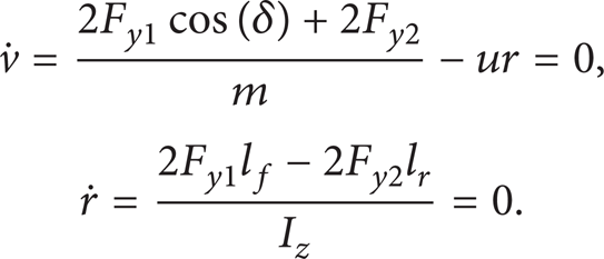
Under such hypotheses, the lateral and yaw vehicle motion equations derived from this simplified vehicle model with nonlinear tire force characteristics were as follows.

The equation of lateral motion of vehicle system was shown as follows:

m (\dot{v} + u r) = 2 F_{y 1} \cos (δ) + 2 F_{y 2},

(2)

where m was vehicle mass, v was the lateral speed, r was the yaw rate, subscripts 1 and 2, respectively, referred to the front and rear axle, andF_yi was the lateral force on the ith axle.

The equation of yaw motion of vehicle system was shown as follows:

I_{z} \dot{r} = 2 F_{y 1} l_{f} - 2 F_{y 2} l_{r},

(3)

where l_f and l_r, were, respectively, the horizontal distances from the front and rear axle to the vehicle's mass center and I_z was the moment of inertia of the vehicle around the vertical axis at the center of gravity. All the vehicle parameters were from the literature [13]. The vehicle parameters were listed in Table 1.

Table 1:

Parameter values of the vehicle model used in this paper.

Mass	m	1640 kg
Moment of inertia around the vertical axis	I _z	2900 kg·m²
Wheelbase	l	2.5 m
Distance of the front axle center from the center of mass	l _f	1.1 m
Distance of the rear axle center from the center of mass	l _r	1.4 m

The kinematic variables of vehicle system (seen in Figure 1) were related by the following:

\begin{matrix} α_{f} = δ - ta n^{- 1} (\frac{v + r \cdot l_{f}}{u}) \approx δ - β - \frac{r \cdot l_{f}}{u}, \\ α_{r} = - ta n^{- 1} (\frac{v - r \cdot l_{r}}{u}) \approx - β + \frac{r \cdot l_{r}}{u} . \end{matrix}

(4)

The lateral tire forces F_yi (i = 1, 2) could be expressed as functions of slip angles α_i (i = 1,2) [14 –16], which were nonlinear and took the below analytical form as follows:

F_{y i} = D_{i} \sin (C_{i} \arctan (B_{i} α_{i} - E_{i} \times (B_{i} α_{i} - \arctan (B_{i} α_{i})))),

(5)

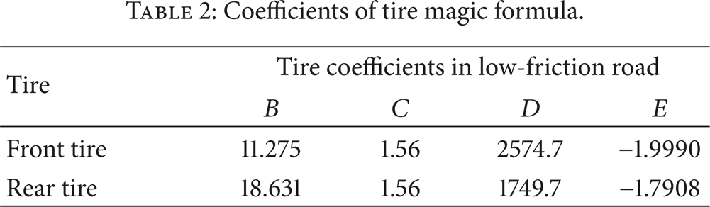
where B_i, C_i, D_i, and E_i (i = 1, 2) were the coefficients of tire magic formula. α_i (i = 1, 2) was the side slip angle. The coefficient values were listed in Table 2, which could represent the tire characteristic in the low-friction road.

Table 2:

Coefficients of tire magic formula.

Tire	Tire coefficients in low-friction road
Tire	B	C	D	E

Front tire	11.275	1.56	2574.7	−1.9990
Rear tire	18.631	1.56	1749.7	−1.7908

The relationship between side slip angle and lateral tire force using tire parameters in Table 2 were graphically shown in Figure 2, which had nonlinear characteristics. The blue line was the relationship of side slip angle and lateral force of front tire and the red one was the relationship of side slip angle and lateral force of rear tire.

Figure 2:

Nonlinear characteristics of lateral tire force.

3. Computation of Equilibrium Points Using Genetic Algorithm

Phase plane analysis was one of the most important techniques for studying the motion characteristics of nonlinear systems, since there was usually no analytical solution for a nonlinear system. Nonlinear systems often had multiple steady-state solutions (namely, equilibrium points). Phase plane analysis of nonlinear systems provided an intuitive and simple way to analyze the steady-state solution that a particular set of initial conditions would converge to [17]. On one hand, the equilibrium points determined the stability characteristic of nonlinear system; the distance between two unstable equilibrium points stood for the boundary of the stable region of nonlinear system. On another hand, the equilibrium points of nonlinear system varied with its parameters and this had a great effect on the stability characteristic of the nonlinear system. Hence, we should not only learn the variation characteristic of equilibrium points of system, but also quantitatively analyze the difference of the equilibrium points of system under different operating conditions.

If the dynamics of a nonlinear system was described by a set of differential equations, the equilibrium points could be estimated by setting all the derivatives to zero. Regarding vehicle dynamics model used in this paper, its equilibrium points could be obtained by setting all the state variables of vehicle system to zero as follows:

\begin{matrix} \dot{v} = \frac{2 F_{y 1} \cos (δ) + 2 F_{y 2}}{m} - u r = 0, \\ \dot{r} = \frac{2 F_{y 1} l_{f} - 2 F_{y 2} l_{r}}{I_{z}} = 0 . \end{matrix}

(6)

In this paper, the tire magic formula was embedded in the vehicle model that contained many nonlinear terms and the conventional numerical computation method, such as Newton Method, to compute the equilibrium points of system demanded that the analytical equations of system were continuous and derivative, so the conventional numerical method was not effective for nonlinear vehicle system. Genetic algorithm was an efficient way to deal with such complex nonlinear problems, which had been wildly used in many practical engineering problems. It was used to figure out the equilibrium points of vehicle model including nonlinear tire characteristic here. The schematic diagram of GA to compute the equilibrium points of vehicle model was shown in Figure 3.

Figure 3:

Schematic diagram of GA for the equilibrium points of vehicle system.

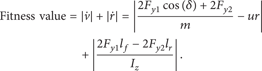
The computing process was finished in the GA toolbox of MATLAB. The parameters of GA were as follows: population size equals 20, itemax equals 500, errmin equals 0.002, and the fitness function was

Fitness value = | \dot{v} | + | \dot{r} | = | \frac{2 F_{y 1} \cos (δ) + 2 F_{y 2}}{m} - u r | + | \frac{2 F_{y 1} l_{f} - 2 F_{y 2} l_{r}}{I_{z}} | .

(7)

4. Bifurcation Characteristics of Vehicle System

The bifurcation analysis was a powerful tool of nonlinear system theory aimed at analyzing and classifying the behaviors of a nonlinear system when one or more state parameters were varied [18]. Typically, the analysis started by studying equilibrium points and by deriving the dependence of its coordinates on a parameter. In doing so, a bifurcation, namely, a structural change in the system behavior, was possibly detected. By systematically analyzing all the equilibrium points, the admissible state parameters' values were eventually derived.

4.1. Bifurcation Analysis with Variation of Vehicle Speed

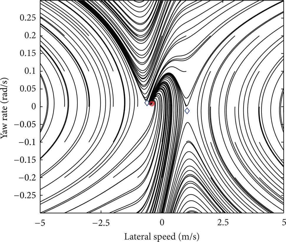
By using the above-mentioned vehicle and tire model, a phase portrait of vehicle system constructed at a slow speed (10 m/s) and steering angle (0.01 rad) of front wheel was shown in Figure 4. The trajectories of vehicle originated at many different initial state variables and propagated through time. Three equilibrium points were identified and two of them were determined to be saddle points, while the other was a stable point [1, 19]. The saddle points were marked by blue diamonds and the stable points were marked by a red circle. All the homoclinic orbits of vehicle system were also shown in Figure 4. The stable manifolds of the saddle points were significant, because they defined the regions of attraction of the stable point.

Figure 4:

Phase portrait at v = 10 m/s and δ = 0.01 rad.

A phase plot of vehicle system constructed at a higher speed of 15 m/s and a steering angle (0.01 rad) of front wheel was shown in Figure 5. All three equilibrium points remained, but the stable point and saddle points had moved toward each other. The boundary of attraction region of vehicle system also moved toward the stable equilibrium point. The attraction region of vehicle was decreased.

Figure 5:

Phase portrait at v = 15 m/s and δ = 0.01 rad.

When the vehicle speed was increased to 30 m/s, the stable point and one saddle point of vehicle system merged and disappeared, as shown in Figure 6. There was no steady-state operation region of vehicle at this speed and the vehicle was out of control.

Figure 6:

Phase portrait at v = 30 m/s and δ = 0.01 rad.

The equilibrium points of vehicle system at different operating conditions were obtained using GA as shown in Figure 7. The bifurcation diagrams of lateral speed and yaw rate versus vehicle speed were shown in Figure 7. We could see that when the vehicle speed was increased to 18.5 m/s at steering angle of front wheel being 0.01 rad, the stable equilibrium point and one saddle point of vehicle system merged and the vehicle system became totally out of control.

Figure 7:

Bifurcation diagrams of the vehicle system under different operating conditions.

4.2. Bifurcation Analysis with Variation of Steering Angle of Front Wheel

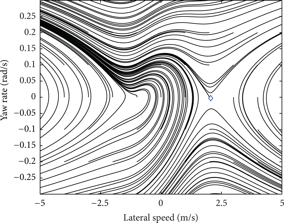
By using the above-mentioned vehicle and tire model, the phase portrait of vehicle system was constructed as the steering angle of front wheel δ were, respectively, set to 0.01, 0.015, and 0.04 rad and vehicle speed was 15 m/s. Figures 8~10 showed the phase plane trajectory of vehicle on v_y-γ plane. Based on the simulation results, it could be concluded that the equilibrium points of vehicle system varied with the steering angle of front wheel. In Figure 8, three equilibrium points were identified and two of them were determined to be saddle points while the other one was a stable point. All the homoclinic orbits of vehicle system were also shown. The attraction region could be figured out, as shown in Figure 8. In Figure 9, all three equilibrium points remained, but the stable point and one saddle point had moved toward each other. The boundary of attraction region of vehicle system also moved toward the stable equilibrium point. The attraction region of vehicle system became smaller and smaller as the steering angle of front wheel increased. In Figure 10, when the steering angle of front wheel was set to 0.04 rad, the stable equilibrium point and one saddle point of vehicle system merged and disappeared. The vehicle was totally out of control.

Figure 8:

Phase portrait at δ = 0.01 rad and v = 15 m/s.

Figure 9:

Phase portrait at δ = 0.015 rad and v = 15 m/s.

Figure 10:

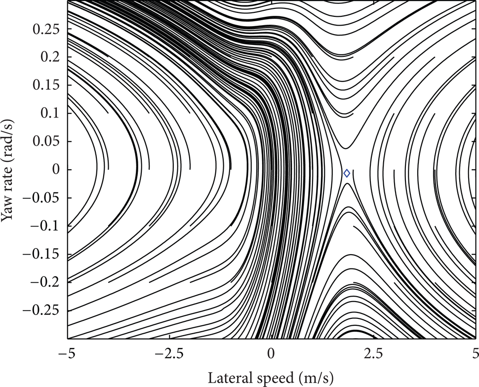
Phase portrait at δ = 0.040 rad and v = 15 m/s.

The bifurcation diagrams shown in Figure 11 illustrated the inherent characteristics of vehicle system as the vehicle speed was constant 15 m/s and the steering angle of front wheel was used as a control parameter of vehicle system. Based on the simulation results, once the front wheel steering angle reached or was beyond 0.012 rad, the stable equilibrium points of vehicle system would disappear and the vehicle system would be out of control.

Figure 11:

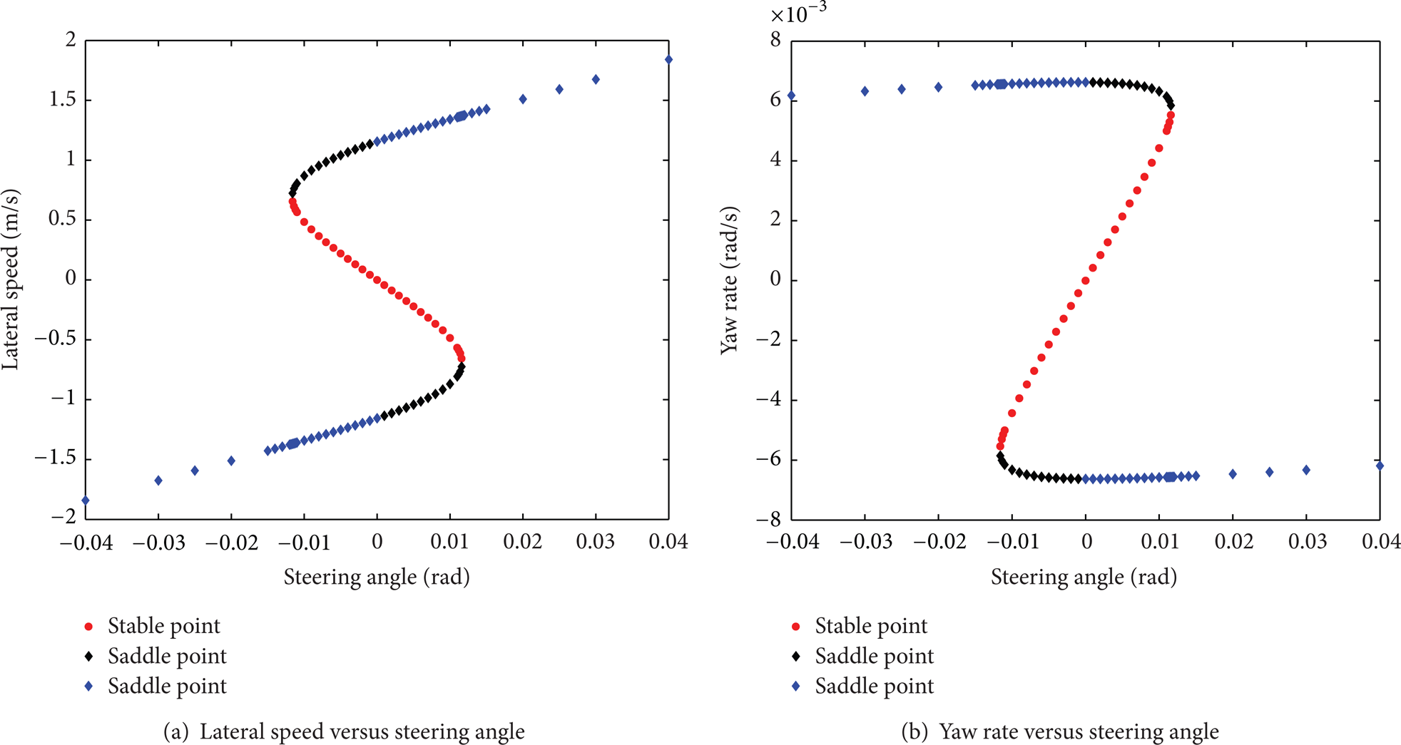
Bifurcation diagrams for the vehicle system under different operating condition.

5. Further Discussion for Plane Motion of Vehicle

In order to understand more about the dynamic behaviors of vehicle negotiating a curve in low-friction road, a series of numerical simulations from (2)~(3) were performed under constant velocity and steering angle of front wheel. Each simulation was characterized by a phase portrait and the plots of state variables (lateral speed v_y and yaw rate γ) of vehicle system over time. Figure 12 showed the dynamic characteristic of vehicle model as the longitudinal speed was set to 15 m/s and the front wheel steering angle was set to 0.01 rad. According to the phase portrait of vehicle state variables (seen in Figure 12 (a)), we could see that the vehicle reached a stable state. From Figure 12 (b), it could be confirmed that the state variables of vehicle remained unchanged over time after five seconds [20], which illustrated that the vehicle system was stable.

Figure 12:

v_x = 15 m/s and δ = 0.01 rad and phase portrait and state variations.

Figure 13 showed the dynamic behavior of vehicle system while the longitudinal speed was set to 15 m/s and the front wheel steering angle was set to 0.04 rad. According to Figure 13 (a), we could see that there was no fixed point in the phase portrait of vehicle state variables. From Figure 13 (b), the absolute values of vehicle state variables kept growing, which illustrated that the vehicle happened to slew and was totally out of control.

Figure 13:

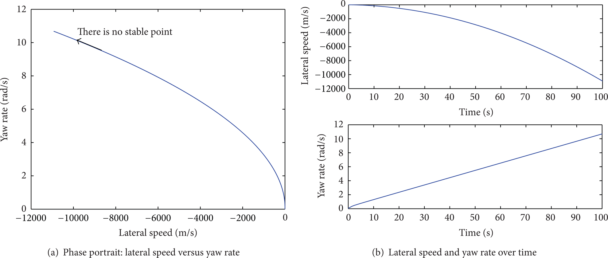
v_x = 15 m/s and δ = 0.04 rad and phase portrait and state variations.

Figure 14 showed the trajectory of vehicle motion in x-y plane as the front wheel steering angle was, respectively, set to 0.01 and 0.04 rad. When the steering angle of front tire equaled 0.01 rad, the vehicle was in a stable motion. When the steering angle of front wheel was increased to 0.04 rad, the radius of vehicle motion kept increasing. It further confirmed that the vehicle happened to slew and was in an unstable motion.

Figure 14:

δ = 0.01 and 0.04 rad and vehicle trajectories in x-y plane.

Figure 15 showed the diagram of lateral tire force versus tire side slip angle, while the vehicle was under different operating conditions. It could be obtained that when the steering angle of front wheel was small and the lateral force of tire was working in the linear region, as shown in Figure 15 (a). However, the tire clearly worked in the nonlinear region, when the front wheel steering angle was increased to 0.04 rad. It could be concluded that working in the nonlinear region of tire was the ultimate reason of vehicle losing its stability.

Figure 15:

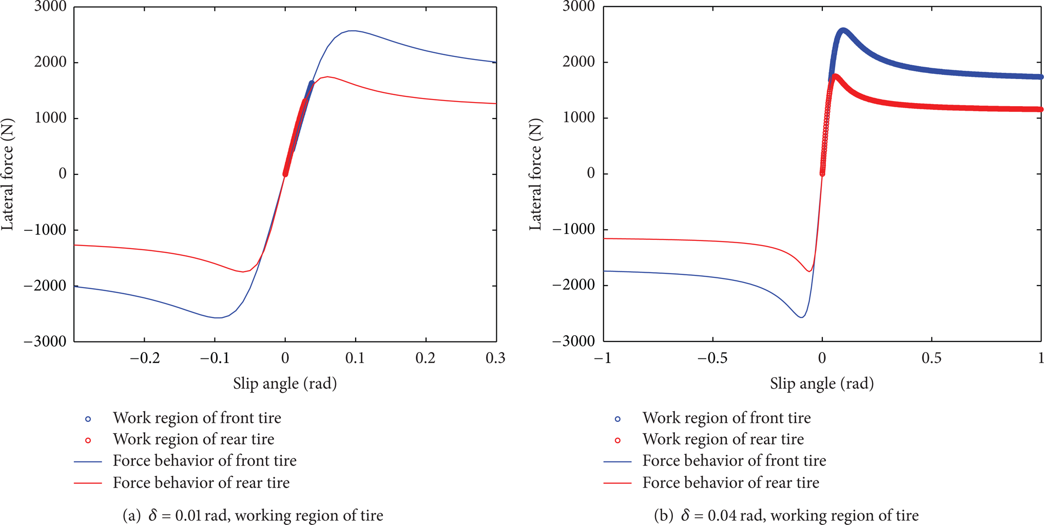
Tire side slip angle and lateral force with δ being 0.01 and 0.04 rad.

6. Conclusion

The nonlinear dynamics behavior of a vehicle cornering on an even low-friction road had been studied through simulation. The simplified vehicle model with two DOFs was built up. The nonlinear tire characteristic was expressed by magic formula.

The phase plane and bifurcation analysis were employed to analyze the motion characteristics of vehicle system under different conditions. To solve out the equilibrium points of vehicle system, the genetic algorithm was introduced to figure out the equilibrium points of vehicle model under different operating conditions.

The stability analysis was conducted by varying two driver's input, namely, the vehicle velocity and the steering angle of front wheel, using phase plane method. The bifurcation behavior of vehicle was observed under different operating conditions. When the steering angle of front wheel was constant being 0.01 rad and the vehicle speed was increased to 18.5 m/s, the stable equilibrium point and one saddle point of vehicle system merged and the vehicle system became totally out of control. When the vehicle was a constant 15 m/sand the front wheel steering angle reached orwas beyond 0.012 rad, the stable equilibrium points of vehicle system would disappear and the vehicle system would be out of control.

To analyze the instability mechanism of vehicle system, the distribution of lateral forces of front and rear tire had been investigated under different operating conditions. When the vehicle was stable, tire was working in the linear region. When the vehicle was unstable, tire was working in the nonlinear region. It could be concluded that working in the nonlinear region of tire was the ultimate reason of the loss of stabilization of vehicle.

The research results could enhance the understanding of vehicle dynamics and be informative for the designers of vehicle control system who have to deal with the active safety of vehicle.

Conflict of Interests

The authors declare that there is no conflict of interests regarding the publication of this paper.

Footnotes

Acknowledgments

This research was supported by a Grant from the National Natural Science Foundation of China (Project no. 51308250), China Postdoctoral Science Foundation (Project no. 2013M530984) and Open Fund of Key Laboratory of Xihua University (Project no. s2jj2012-038).

References

Nguyen

Schultz

, and Balachandran

, “Lateral load transfer effects on bifurcation behavior of four-wheel vehicle system,” Journal of Computational and Nonlinear Dynamics, vol. 4, no. 4, pp. 1–12, 2009.

Chang

S.-C.

, “Synchronization in a steer-by-wire vehicle dynamic system,” International Journal of Engineering Science, vol.45, no. 2–8, pp. 628–643, 2007.

Harada

and Harada

, “Analysis of lateral stability with integrated control of suspension and steering systems,” JSAE review, vol. 20, no. 4, pp. 465–470, 1999.

You

S.-S.

and Jeong

S.-K.

, “Controller design and analysis for automatic steering of passenger cars,” Mechatronics, vol. 12, no. 3, pp. 427–446, 2002.

Shen

Wang

Shi

, and Premier

, “Nonlinear dynamics and stability analysis of vehicle plane motions,” Vehicle System Dynamics, vol. 45, no. 1, pp. 15–35, 2007.

Inagaki

Kshiro

, and Yamamoto

, “Analysis of vehicle stability in critical cornering using phase plane method,” SAE Paper 943841, 1994.

Ono

Hosoe

Tuan

H. D.

, and Doi

, “Bifurcation in vehicle dynamics and robust front wheel steering control,” IEEE Transactions on Control Systems Technology, vol. 6, no. 3, pp. 412–420, 1998.

Catino

Santini

, and di Bernardo

, “MCS adaptive control of vehicle dynamics: an application of bifurcation techniques to control system design,” in Proceedings of the 42nd IEEE Conference on Decision and Control, pp. 2252–2257, December 2003.

Lukowski

Momot

Kraemer

, and Kunz

, “Basic linear theory of handling and stability of automobiles,” Proceedings of the Institution of Mechanical Engineers D, vol. 223, no. 1, pp. 1–10, 2009.

10.

Dai

and Han

, “Stability and Hopf bifurcation of a nonlinear model for a four-wheel-steering vehicle system,” Communications in Nonlinear Science and Numerical Simulation, vol. 9, no. 3, pp. 331–341, 2004.

11.

Hegazy

Rahnejat

, and Hussain

, “Multi-body dynamics in full-vehicle handling analysis under transient manoeuvre,” Vehicle System Dynamics, vol. 34, no. 1, pp. 1–24, 2000.

12.

Liu

Shi

Shen

, and Chu

, “Vehicle planar motion stability study for tyres working in extremely nonlinear region,” Chinese Journal of Mechanical Engineering, vol. 23, no. 2, pp. 185–194, 2010.

13.

Hao

and Xian-sheng

, “Phase plane analysis for vehicle handling and stability,” International Journal of Computational Intelligence Systems, vol. 4, no. 6, pp. 1179–1186, 2011.

14.

Cabrera

J. A.

Ortiz

Carabias

, and Simon

, “An alternative method to determine the magic tyre model parameters using genetic algorithms,” Vehicle System Dynamics, vol. 41, no. 2, pp. 109–127, 2004.

15.

Bakker

Pacejka

H. B.

, and Lidner

, “A new tire model with an application in vehicle dynamics studies,” SAE Paper 890087.

16.

Gim

and Nikravesh

P. E.

, “Analytical model of pneumatic tyres for vehicle dynamic simulations. Part 1. Pure slips,” International Journal of Vehicle Design, vol. 11, no. 6, pp. 65–75, 1990.

17.

Rossa

F. D.

Mastinu

, and Piccardi

, “Bifurcation analysis of an automobile model negotiating a curve,” Vehicle System Dynamics, vol. 50, no. 8, pp. 1–24, 2012.

18.