Error Correction for Laser Tracking System Using Dynamic Weighting Model

Abstract

Laser tracking system (LTS) has been widely used in energy industries to meet increasingly high accuracy requirements. However, its measuring accuracy is highly affected by the dynamic uncertainty errors of LTS, and also the current range and angle measurements of LTS are mainly weighted statically, obtaining the dynamic weighting model which is essential for LTS to improve the measuring accuracy. In this paper, a dynamic weighting model that describes not only the dynamic uncertainty but also the geometric variations of LTS is developed, which can be adjusted to the weighting factors of dynamic parameters according to the range observations relative to the angle observations. Intensive experimental studies are conducted to check validity of the theoretical results. The results show that the measuring accuracy of LTS has been increased 2 times after using this technique for correction.

1. Introduction

Conventional coordinate measuring machines (CMMs), as one of the powerful measuring instruments, have been widely used for dimensional and geometrical inspection in manufacturing industry for the past few decades. However, conventional CMMs are not appropriate when measuring large components (typical size from 5 m to 100 m). In addition, in some cases, it is not possible or necessary to bring the parts onto the CMMs. Therefore, mobile large scale metrological instruments are being used to meet these requirements. Among a broad range of large scale measuring systems, such as optical scanner, laser radar, indoor GPS, and digital photogrammetry, laser tracking system (LTS) has become the backbone for accurate dimensional measurement in many industrial and scientific fields due to its high accuracy, large measuring range, high sampling rate, and automatic target tracking. It has been widely used in manufacturing measurement for dimension inspection, robot calibration, machine alignment, surface contour mapping, and reverse engineering [1–7].

The LTS is an integrated measuring system with optical, mechanical, and electronic components. The errors from these components, together with the environmental and operational factors, determine the measurement uncertainty of the LTS. This paper classifies uncertainty sources in LTS measurement into two categories, namely, static or quasistatic uncertainty sources and dynamic uncertainty sources. In order to improve the LTS measuring accuracy and reduce the uncertainty sources, Umetsu et al. [8] proposed a novel method for error analysis and self-calibration of laser tracking mirror mechanism in LTS and developed a kinematics model of geometric variations for LTS. Liu and Wang [9–11] have described the misalignments for the laser tracker design that uses a gimbaled mirror for beam steering. The 15 parameters of their model are broadly categorized as offsets, tilt deviations, and angle encoder parameters. Manojlović and Lin [12, 13] derived formulae to correct the observed sensor readings for the influence of these error parameters and describe experimental setups that can be deployed to measure the error parameters of laser tracker. Muralikrishnan et al. modeled a laser tracker in which the laser beam source is inside the rotating head—this design does not require use of a gimbaled mirror. Bai and Wang [14] develop the dynamic model of the tracking gimbals of LTS using the Lagrange-Euler equations.

However, all the above researches are mainly focusing on static or quasi-static uncertainty models of LTS; the dynamic uncertainty sources are also highly affected by the LTS measuring accuracy, obtaining the dynamic weighting model which is essential for LTS to improve the measuring accuracy. Therefore, this paper developed a dynamic weighting model of LTS, which can be adjusted to the weighting factors of dynamic parameters according to the range observations relative to the angle observations. A virtual and real measured integration method is presented to correct LTS measurements with dynamic weighting model. The technique can be used to perform error correction for LTS and also to determine all parameters of the dynamic weighting model.

2. Working Principle of LTS

The LTS measuring principle is based on a spherical coordinate system; it can be regarded as a portable frameless coordinate measuring machine. The LTS includes a tracking mirror mechanism, a motor control unit, a laser interferometer, a retroreflector, and a position detector; the working principle of LTS is shown in Figure 1.

Figure 1:

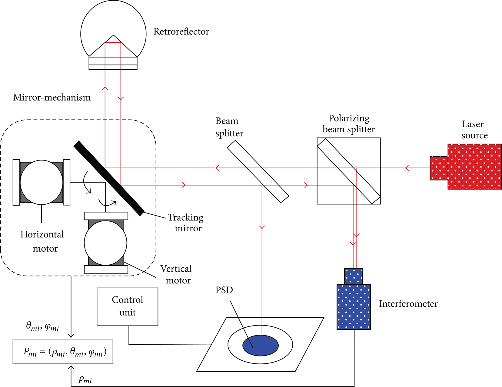
Working principle of LTS.

Firstly, the laser source emits a measuring laser beam, when the measuring laser beam passes through the beam splitter. Secondly, a portion of measuring laser beam is directed to the retroreflector by a 2-axis tracking mirror mechanism. Another portion of the return beam is directed by a beam splitter onto a 2-dimensional position sensitive detector (PSD) that senses lateral motion of the target reflector. An interferometer measures the target retroreflector linear displacement. 2-axis high-resolution angle encoders provide the horizontal and vertical angles (θ, φ) of a spherical coordinate system. Finally, the displacement interferometer provides the radial coordinate ρ of the target center. The resultant error signal is used by motor control unit under a certain control algorithm to drive the tracking mirror mechanism so that the displacement measuring beam remains centered on the target as it moves through the space. When the initial optical path between the center of the mirror and the home position is calibrated, the spherical coordinate, P _mi = (ρ _mi , θ _mi , φ _mi ), of the reflector can be obtained in real time from the interferometer and encoder readings.

When LTS is used for high accuracy measurement, its measuring accuracy is highly affected by the dynamic uncertainty errors, obtaining the dynamic weighting model of LTS which is essential prior to using it for metrology.

3. Dynamic Weighting Model

3.1. The Ideal Model of LTS

In this model, it is assumed that the two gimbal axes are intersecting and perpendicular to each other and there is no mirror center offset.

As shown in Figure 2, {x, y, z} is the world coordinate system of LTS. In order to model LTS, the three coordinate systems are established as follows. They are the base coordinate system of the gimbal {x _b , y _b , z _b }, the first link frame {x₁, y₁, z₁} and the mirror frame {x _m , y _m , z _m }. The origins of three frames are placed at the mirror center C. z _b is the rotation axis of the first joint, z₁ is the rotation axis of the second joint, and x _m is normal to the mirror surface. When the gimbal is at its home position (θ₁ = θ₂ = 0), the x-axes of the first two frames are coincident with the mirror surface normal; b _i represents the direction of the laser beam hitting on the mirror surface, b _c represents the direction of the mirror surface normal, and b _o represents the direction of the laser beam reflected from the mirror surface.

Figure 2:

Ideal model of LTS.

Coordinate system {x _b , y _b , z _b } can be brought to coordinate system {x _m , y _m , z _m } by the following sequence of 4 × 4 homogeneous transformations:

${}^b{T}_m=\mathrm{rot}\left(z,{\theta }_1\right)\mathrm{rot}\left(x,-{90}^{°}\right)\mathrm{rot}\left(z,{\theta }_2\right)\mathrm{rot}\left(x,{90}^{°}\right).$

(1)

Thus the mirror surface normal b _c = (b _cx , b _cy , b _cz ) ^T represented in {x _b , y _b , z _b } is obtained from the three elements of the third column of ${}_{}{}^b{T}_m$ by

$\begin{array}{l}{b}_{cx}=\cos {\theta }_{\mathrm{1}}\cos {\theta }_{\mathrm{2}},\\ b_{cy}=\sin {\theta }_{\mathrm{1}}\cos {\theta }_{\mathrm{2}},\\ b_{cz}=\sin {\theta }_{\mathrm{2}}.\end{array}$

(2)

The direction of the incident beam is fixed, but that of the reflected beam varies with the position of the retroreflector. If the directions of the incident beam and the surface normal of the mirror are known, the direction of the reflected beam can be got by using the following formula:

$b_o=-B\left(b_c\right)b_i,$

(3)

where $B(b_c)=\left(\begin{array}{ccc}2b_{cx}^2-1& 2b_{cx}{b}_{cy}& 2b_{cx}{b}_{cz}\\ 2b_{cx}{b}_{cy}& 2b_{cy}^2-1& 2b_{cy}{b}_{cz}\\ 2b_{cx}{b}_{cz}& 2b_{cy}{b}_{cz}& 2b_{cz}^2-1\end{array}\right)$ is the familiar of the mirror image reflection matrix [15].

Let R be a reference target point at which θ₁ = θ₂ = 0. If the distance between the mirror center and the retroreflector is known, the location r _P of the retroreflector at any point P can be computed by the following formula:

$r_P=l{b}_o=\left(l_m+l_r\right)b_o=\left(l_m+l_r\right)B\left(b_c\right)b_i,$

(4)

where l is the distance from the point at which the incident beam hits the mirror surface (point C in this ideal case) to the target location, l _m is the relative distance measured by the laser interferometer, and l _r is the distance from the reference point to point C.

To compute the target location r _P , the parameters l _r and b _i need to be obtained by calibration. l _m , θ₁, and θ₂ are provided by distance and angular measurements of the laser tracker, and b _c is computed by (2) using the measured θ₁ and θ₂.

3.2. Mirror Center Offset Model

Section 3.1 has described an ideal model, in assumption, without mirror center offset and gimbal axis misalignment. This model can be extended to include nonzero mirror center offset under assumption of perpendicularly intersecting mirror gimbal axis. c _r and c represent intersecting points between laser beam and mirror surface; c _m is the rotational point of mirror.

Figure 3 illustrates the LTS with mirror center offset; b _or and b _cr are the mirror surface normal and the direction of the reflected beam, respectively, when the retroreflector is at r _r . Similarly b _o and b _c are the vectors when the retroreflector is at r _P and b _i represents the direction of the laser beam hitting on the mirror surface.

Figure 3:

Mirror center offset model of LTS.

Based on the 3D geometry of the system, the retroreflector coordinates can be computed by the following formula:

$r_P=R_r^{}{}^m{c}_r-\left(l_m+l_r-l_s\right)B\left(b_c\right)b_i+l_s{b}_i,$

(5)

where $l_s=-b_c·(R^{}{}^m{c}_r)/b_c·b_i$ , R _r is the rotation submatrix of T _m (refer to (2)), when θ₁ = θ₂ = 0. Consider ${}^m{c}_r={(c_x,c_y,0)}^T$ ; c _x and c _y are the two parameters describing the mirror center offset. The rest of variables are the same as those in the last section.

3.3. Combined Mirror Center Offset and Gimbal Axis Misalignments Model

Calibration considerations of LTS must be taken into account during the modeling process of the gimbal-mirror mechanism. Compared with the model presented in the previous section, the new model should include both mirror center offset and gimbal axis misalignment. It is a complete and minimal model because it satisfies the two basic requirements. Firstly, there should be a sufficient number of kinematic parameters to completely describe the geometry and motion of the actual gimbal mechanism. Secondly, there should be no redundant parameters in the parameter identification process.

As shown in Figure 4, O _b , O₁, and O _m denote the origins of the three coordinate systems {x _b , y _b , z _b }, {x₁, y₁, z₁}, and {x _m , y _m , z _m }, respectively. When the LTS is at its home position, x _b and x₁ are along the common normal directions of z _b and z₁. If z _b and z₁ intersect, x _b and x₁ are assigned perpendicular to both z _b and z₁. Let O _b and O₁ are the intersection points of the common normal of axes z _b and z₁with x _b and x₁, respectively. Thus an angular parameter α₁ and a translation a₁ are used to model the misalignment of the gimbal axes. Therefore, rot(x, α₁) will align {x _b , y _b , z _b } with {x₁, y₁, z₁}, and tran(a₁, 0,0) will bring the resultant frame to be coincident with {x₁, y₁, z₁}. x _m is parallel to the direction of the mirror surface normal and passes through O₁. O _m is the intersection point of x _m with the mirror surface. z _m may lie arbitrarily on the mirror surface. Two angular parameters θ₂ and α₂ as well as one translation parameter e₂ are thus sufficient to model the case, in which the second rotation axis does not lie on the mirror surface. In other words, rot(z, θ₂ + Δθ₂)rot(x, α₂) will align {x₁, y₁, z₁} with {x _m , y _m , z _m }, and tran(0,0, e₂) will bring the result frame to be coincident with {x _m , y _m , z _m }.

Figure 4:

Mirror center offset and gimbal axis misalignment model.

In summary, the transformation matrix ${}_{}{}^b{T}_m$ relating the coordinate system {x _m , y _m , z _m } to {x _b , y _b , z _b } is

${}_{}{}^b{T}_m=\mathrm{rot}(z,{\theta }_1)\mathrm{rot}(x,{\alpha }_1)\mathrm{tran}(a_1,\mathrm{0,0})\times \mathrm{rot}\left(z,{\theta }_2\right)\mathrm{rot}\left(x,{\alpha }_2\right)\mathrm{tran}\left(\mathrm{0,0},e_2\right),$

(6)

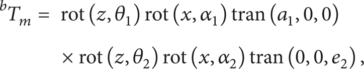
nominally α₁ = – 90°, α₂ = 90°, and e₂ = 0.

The target coordinates can be computed through the following formula:

$r_P=R_r^{}{}^m{c}_r+t_r-\left(l_m+l_r-l_s\right)B\left(b_c\right)b_i+l_s{b}_i,$

(7)

where $l_s=-b_c·(R{}^m{c}_r)/b_c·b_i$ .

3.4. Dynamic Weighting Model with Mirror Center Offset and Gimbal Axis Misalignments

It is difficult to predict how a given set of dynamic uncertainty sources will affect the range and angle measurements of LTS, and there is good reason to believe that the effect on range measurements will be different to that on the angle measurements. Therefore, it is necessary to obtain the dynamic weighting model with mirror center offset and gimbal axis misalignments of LTS for metrology.

Section 3.3 has described the target coordinates $r_P={[\rho ,\theta ,\phi ]}^T$ ; it is assumed that the true measured ranges and azimuth and elevation angles ρ^*, θ^*, and φ^* arise through a sampling model of the form

$\begin{array}{c}{\rho }^{*}=\rho (x,S)+{\epsilon }_{\rho },\\ {\theta }^{*}=\theta (x,S)+{\epsilon }_{\theta },\\ {\phi }^{*}=\phi \left(x,S\right)+{\epsilon }_{\phi },\end{array}$

(8)

where x and S are fixed but to the target locations and static or quasi-static uncertainty parameters, respectively, and ε_ρ, ε_θ and ε_φ are samples from a dynamic uncertainty distribution with expectation zero and standard deviations σ_ρ, σ_θ and σ_φ, respectively. We assume that these standard deviations reflect an uncertainty component that is independent of the distance to the target. The quantities ρ^*, θ^*, and φ^* are what the model predicts the LTS measurements should be. For a given target x, we assume that

${\sigma }_{\rho }^2={\sigma }_{\rho ,S}^2+{\sigma }_{\rho ,D}^2{\parallel {\epsilon }_{\rho }\parallel }^2,$

(9)

where σ_{ρ, S}, σ_{ρ, D} are the static and dynamic standard deviations of ρ^*.

The uncertainty associated with the displacement measurement, potentially, has a component dependent on the dynamic uncertainty from the LTS to the target. The dynamic uncertainty dependence could arise from the retroreflector moving velocity or acceleration, or random fluctuations in the refractive index, or random effects associated with the laser frequency, for example. The dynamical characterization is used to weight the displacement measurements with ω_ρ = 1/σ_ρ. In practice, the observed ρ^* can be used as an estimate of $\parallel {\epsilon }_{\rho }\parallel$ so that

${\omega }_{\rho }=\frac{1}{\sqrt{{\sigma }_{\rho ,S}^2+{\sigma }_{\rho ,D}^2{\parallel {\epsilon }_{\rho }\parallel }^2}}.$

(10)

For azimuth angle observations, the statistical characterization has the form of equation (8); the ε_θ is a realization of a random variable with expectation zero and variance σ_θ². We assume that, for each measurement, σ_θ depends on two parameters σ_{θ, S} and σ_{θ, D}, with

${\sigma }_{\theta }^2=\frac{1}{{\parallel {\epsilon }_{\rho }\parallel }^2{\cos }^2\theta }\left({\sigma }_{\theta ,D}^2+\frac{{\sigma }_{\theta ,S}^2}{{\parallel {\epsilon }_{\theta }\parallel }^2}\right).$

(11)

The term σ_{θ, D} accounts for random effects associated with the target that will have a larger impact on the angle measurements for targets closer to the station. The dependence of the variance parameter σ_θ² on the azimuth angle θ models the fact that as the targets move away from the equatorial plane, the azimuth angle is less well defined. This leads to assigning weights according to

${\omega }_{\theta }=\frac{\mathrm{1}}{{\sigma }_{\theta }}=\frac{\parallel {\epsilon }_{\theta }\parallel \parallel {\epsilon }_{\rho }\parallel \cos \theta }{\sqrt{{\sigma }_{\theta ,S}^{\mathrm{2}}+{\sigma }_{\theta ,D}^{\mathrm{2}}{\parallel {\epsilon }_{\theta }\parallel }^{\mathrm{2}}}}.$

(12)

Similarly, for elevation angle measurements, the weights characterization has the following:

${\omega }_{\phi }=\frac{\parallel {\epsilon }_{\phi }\parallel \parallel {\epsilon }_{\rho }\parallel \sin \phi }{\sqrt{{\sigma }_{\phi ,S}^2+{\sigma }_{\phi ,D}^2{\parallel {\epsilon }_{\phi }\parallel }^2}}.$

(13)

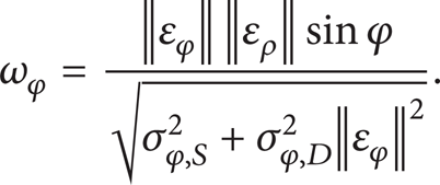
According to (7), (8), (10), (12), and (13), the dynamic weighting model with mirror center offset and gimbal axis misalignments of LTS can be calculated as

$r_P^{*}=r_P+J_i\left(\begin{array}{ccc}{\omega }_{\rho }& & \\ & {\omega }_{\theta }& \\ & & {\omega }_{\phi }\end{array}\right)J_i^T.$

(14)

The Jacobian matrix J _i can be solved by

$\begin{array}{l}{J}_i=\left(\begin{array}{ccc}\frac{\partial x}{\partial \rho }& \frac{\partial x}{\partial \theta }& \frac{\partial x}{\partial \phi }\\ \frac{\partial y}{\partial \rho }& \frac{\partial y}{\partial \theta }& \frac{\partial y}{\partial \phi }\\ \frac{\partial z}{\partial \rho }& \frac{\partial z}{\partial \theta }& \frac{\partial z}{\partial \phi }\end{array}\right)\\ =\left(\begin{array}{ccc}\cos {\theta }_i\sin {\phi }_i& -{\rho }_i\sin {\theta }_i\sin {\phi }_i& {\rho }_i\cos {\theta }_i\cos {\phi }_i\\ \sin {\theta }_i\sin {\phi }_i& {\rho }_i\cos {\theta }_i\sin {\phi }_i& {\rho }_i\sin {\theta }_i\cos {\phi }_i\\ \cos {\phi }_i& \mathrm{0}& -{\rho }_i\sin {\phi }_i\end{array}\right).\end{array}$

(15)

4. Experiments

The objective is to test the feasibility of the proposed method for the purpose of LTS error correction. The r _P and r _P ^* were given in the above section. About a hundred 3D target points were randomly generated in a 1.5 × 1.5 × 1.5 m³ work volume which were assumed to be “trackable” by the LTS system. In order to demonstrate the effectiveness of our proposed technique, we used it to perform a dynamical uncertainty correction of a commercial LTS (FARO SI) shown in Figure 5. The retroreflector is mounted on the z-axis of a CMM. The CMM that rides the retroreflector moves in space to simulate the dynamic constraint of LTS. Based on the nominal values provided by the high-accuracy CMM, the LTS tracks the retroreflector and measures the coordinates of the retroreflector in real time.

Figure 5:

Experiment layouts.

In the experiments, 100 points are measured with the dynamic constraint. Figure 6 shows the measuring results using our proposed technique. The horizontal axis represents the number of measurements and the vertical axis denotes the measuring error relevant to the standard value provided by CMM. The black line is the results, in which LTS has not been calibrated by the proposed technique. At the same time, the dash line denotes the results, in which LTS has been calibrated using the proposed technique. After being corrected using dynamic weighting model, the mean measuring error of the LTS has been decreased from 99.57 μm to 53.89 μm.

Figure 6:

Measuring results using dynamic weighting model.

5. Conclusion

The dynamic weighting model that describes not only the dynamic uncertainty but also the geometric variations of LTS is developed, which can be adjusted to the weighting factors of dynamic parameters according to the range observations relative to the angle observations. The experimental results have demonstrated that, using this technique to correct the LTS measuring errors, the maximum value of LTS measurements has been decreased from 99.57 μm to 53.89 μm.