Sage Journals: Discover world-class research

Abstract

We developed a new immersed boundary method which has various advantages, such as accuracy, flexibility, and rapidness combining with the level set method. We numerically demonstrated some typical examples, such as flows around a sphere, an ellipsoid, a flapping ellipsoid, and a windmill. We calculated coefficients of drag in those problems and visualized vortical structures and Powell sound sources for the various Reynolds number and then compared our results with some previous researches.

1. Introduction

In recent years, the development of computer performance has enabled us to conduct numerical simulation of highly complex flow phenomena around a moving object whose shape is quite complicated. So far, various types of calculation grids have been proposed. However, the more grids are complicated, the more calculation time and a required memory increase.

Therefore, we paid our attention to the immersed boundary method (later on we abbreviate it as IB method), which immerses a complicated-shaped boundary at an orthogonal grid system and the level set method which captures any object shape correctly. Although the IB method is a technique proposed by Peskin [1] in 1972, in order to be able to perform highly precise calculation, having a lot of grids with an orthogonal grid system is required. In virtue of improvement in computer performance in recent years, it receives an attracting attention again. On the other hand, the level set method is the technique of capturing any object shape correctly, and now it is used not only in computational fluid dynamics (CFD) but also in the field of image processing. Moreover, it has the advantage that the moving boundary can be tracked with high accuracy.

In this research, we developed the new computational technique which can be applied to the CFD for a moving boundary or a complicated object shape and can carry out numerical computations rapidly by combining the IB method for analyzing complicated form by an orthogonal grid system and the level set method for capturing object shape correctly. We calculated the flow around an object by using the level set IB method and verified the adaptability of the code by changing the Reynolds number. In this research, after computations of the flow around a sphere or an ellipsoid which is stationary or rotates in the uniform flow, then computations of the flow around a moving object in the uniform flow which imitates flapping wings and a windmill are conducted. In addition, in this research, we paid attention to the aeroacoustics, and the aerodynamic sound source was visualized together with the vortical structure and the coefficient of drag.

2. Dimensionless Equations

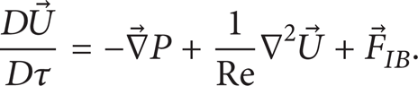
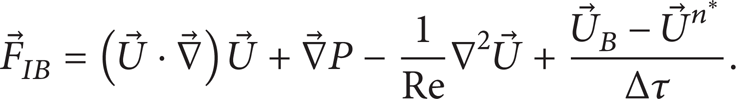
The dimensionless equations used in this research are as follows. In addition, since the IB method is used, the velocity of an object-inside point and of a boundary adjacent point is corrected by external force term ${\vec{F}}_{I B}$ .

(i) Equation of continuity:

\vec{\nabla} \cdot \vec{U} = 0 .

(1)

(ii) Navier-Stokes equation:

\frac{D \vec{U}}{D τ} = - \vec{\nabla} P + \frac{1}{Re} \nabla^{2} \vec{U} + {\vec{F}}_{I B} .

(2)

A boundary adjacent point $(\vec{U} = {\vec{U}}_{I B})$ :

{\vec{F}}_{I B} = (\vec{U} \cdot \vec{\nabla}) \vec{U} + \vec{\nabla} P - \frac{1}{Re} \nabla^{2} \vec{U} + \frac{{\vec{U}}_{I B} - {\vec{U}}^{n^{*}}}{Δ τ} .

(3)

An object-outside point:

{\vec{F}}_{I B} = \vec{0} .

(4)

An object-inside point $(\vec{U} = {\vec{U}}_{B})$ :

{\vec{F}}_{I B} = (\vec{U} \cdot \vec{\nabla}) \vec{U} + \vec{\nabla} P - \frac{1}{Re} \nabla^{2} \vec{U} + \frac{{\vec{U}}_{B} - {\vec{U}}^{n^{*}}}{Δ τ} .

(5)

Velocity ${\vec{U}}_{I B}$ is a velocity given by the level set method, and ${\vec{U}}_{B}$ is an object-inside velocity. Besides, the Reynolds number of uniform flow is set to Re, and Reynolds number resulting from rotation and flapping is denoted to Re_r.

3. Immersed Boundary Method and Level Set Method

Although various kinds of approximated methods are proposed for the IB method, in this study, we approximate it by using the distance function called a level set function (ϕ), which was first introduced in the IB method by the study of Okita et al. [2]; also the study which used level set IB method to a moving boundary is introduced by Sato [3]. As shown in Figure 1, a level set function has the characteristic that the normal distance from a boundary to a grid point is acquired. By calculating the velocity gradients 1 and 2 of two kinds of normal directions ((6) and (7)), the velocity U_IB near the boundary is calculated. The existence of a boundary of object is captured correctly from the information of normal distance ϕ_{I – 1, K} > 0, ϕ_{I + 1, K} < 0 as shown in Figure 2, and bordering curvature is judged from that of ϕ_{I, K + 1} > ϕ_{I, K – 1}. This technique is the level set method, and since a velocity gradient is made as for order to a normal direction by this method, it leads to improvement in arithmetic precision. In this connection, this technique referred to what was invented by Okita et al., and in this study, the technique was extended so that the influence of a normal velocity gradient might be reflected more greatly, and we tried to raise analysis accuracy. Moreover, even when object velocity changes with places like a moving boundary, there is an advantage that the velocity can be acquired easily by using a level set function.

Figure 1:

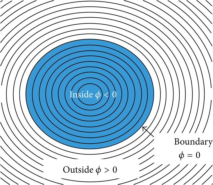
Level set function.

Figure 2:

Boundary adjacent velocities. (U_IB: boundary adjacent velocity, U_B: object inside velocity, ϕ: level set function.) The situation of the horizontal velocity U near the boundary is shown.

(i) Normal velocity gradient 1 (2 dimension):

\begin{matrix} {\frac{\partial U}{\partial n} |}_{I, K} = sgn ({\frac{\partial U}{\partial X} |}_{I, K} n_{X} + {\frac{\partial U}{\partial Z} |}_{I, K} n_{Z}) \cdot \sqrt{{({\frac{\partial U}{\partial X} |}_{I, K} n_{X})}^{2} + {({\frac{\partial U}{\partial Z} |}_{I, K} n_{Z})}^{2}} \\ (n_{X} = \frac{φ_{X}}{\sqrt{φ_{X}^{2} + φ_{Z}^{2}}}, n_{Z} = \frac{φ_{Z}}{\sqrt{φ_{X}^{2} + φ_{Z}^{2}}}, φ_{X} = \frac{\partial φ}{\partial X}, φ_{Z} = \frac{\partial φ}{\partial Z}) . \end{matrix}

(6)

(ii) Normal velocity gradient 2 (2 dimension):

{\frac{\partial U}{\partial n} |}_{I, K} = \frac{U_{I B} - U_{B 2}}{φ_{I, K}} {⟺ U}_{I B} = U_{B 2} + {\frac{\partial U}{\partial n} |}_{I, K} φ_{I, K} .

(7)

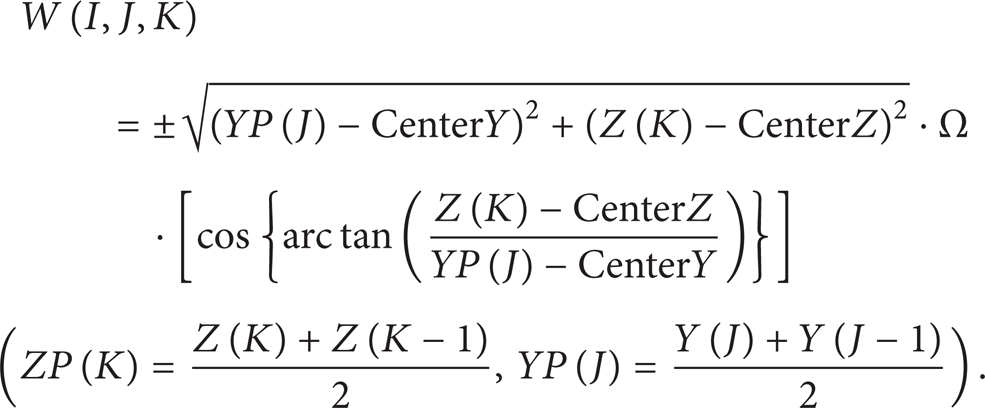
By substituting (6) to (7), the velocity U_IB of a boundary adjacent point is calculated. And we calculate V or W with the same procedure. Besides, in this case, angular velocity is uniform, so the velocity can be found if the distance and angle from the center are known. The velocity inside a moving object is as follows:

U (I, J, K) = 0,

(8)

V (I, J, K) = \pm \sqrt{{(Y (J) - Center Y)}^{2} + {(Z P (K) - Center Z)}^{2}} \cdot Ω \cdot [\sin {arc \tan (\frac{Z P (K) - Center Z}{Y (J) - Center Y})}],

(9)

\begin{matrix} W (I, J, K) = \pm \sqrt{{(Y P (J) - Center Y)}^{2} + {(Z (K) - Center Z)}^{2}} \cdot Ω \cdot [\cos {arc \tan (\frac{Z (K) - Center Z}{Y P (J) - Center Y})}] \\ (Z P (K) = \frac{Z (K) + Z (K - 1)}{2}, Y P (J) = \frac{Y (J) + Y (J - 1)}{2}) . \end{matrix}

(10)

4. Computational Methods

In this research, each analysis assumes the incompressible Newtonian fluid, and the inequality interval staggered grids are used. The difference schemes we use are the third order upwind difference scheme (UTOPIA) for the advection terms of the equation of motion, the Euler explicit method for the time derivative term, and the second order central differences for other terms. And, the SOR method is used for the solution of the Poisson's equation of pressure, and the fractional step method is applied to the algorithm of calculation.

5. Visualization of Sound Source

In this research, a vortical structure by λ2 method, a coefficient of drag, streamlines, and sound source distribution are visualized in each result. Sound source distribution is explained in detail below.

As one of the causes of noise, the aerodynamic noise (aerodynamic sound) which occurs by turbulence of air is often mentioned. Therefore, although it becomes indispensable in acoustical technology to reduce aerodynamic sound, it is difficult to specify a generating part of sound in an experiment for fluid itself. Therefore, we paid attention to the sound source of aerodynamic sound which can investigate the generating part and generation mechanism of sound. The basic equation of aerodynamic sound calculation is the following Lighthill's equation [4]:

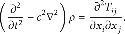
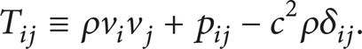
(\frac{\partial^{2}}{\partial t^{2}} - c^{2} \nabla^{2}) ρ = \frac{\partial^{2} T_{i j}}{\partial x_{i} \partial x_{j}} .

(11)

T_ij expresses the following Lighthill turbulent stress tensor

T_{i j} \equiv ρ v_{i} v_{j} + p_{i j} - c^{2} ρ δ_{i j} .

(12)

The left-hand side of (11) expresses propagation of sound, and the right-hand side expresses a sound source. Since this is a nonhomogeneous wave equation, it is difficult to make analysis by DNS calculation, and in this research, the sound source was visualized from the following equation of Powell-Howe [5] which can be used under a flow of low Mach number:

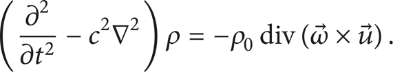
(\frac{\partial^{2}}{\partial t^{2}} - c^{2} \nabla^{2}) ρ = - ρ_{0} div (\vec{ω} \times \vec{u}) .

(13)

Since ρ₀ is standard density and it is fixed, a sound source is given by $div (\vec{ω} \times \vec{u})$ (Powell sound source term) of the right-hand side of (13). After calculating a flow field by a separation solution, a sound source is calculated.

6. Computation around a Rotating Sphere and Ellipsoid

6.1. Computational Conditions

An analysis model is shown in Figure 3. The initial condition assumes external uniform flow (U = 1, V = 0, W = 0, and P = 0) for the whole domain, and the boundary condition is set up as shown in Table 1. The inflow boundary is given by velocity regularity, the outflow boundary is given by the Sommerfeld radiation condition [6], the velocity at the lateral walls is considered as continuation, and the circumference of an object is set as no-slip condition. Characteristic length D is the diameter of a sphere or the short diameter of an ellipsoid. The long diameter of the ellipsoid is extended only to x-axis orientation as 1.5D, and rotation is given with respect to the x-axis. In both analysis of the sphere and the ellipsoid, the number of grids is (X, Y, Z) = (167,138, 138), the calculation area is 8D × 6D × 6D, and the center position of an object is (3D, 3D, 3D). Besides, the computed results are compared with the experimental values which were performed in other researchers by changing Reynolds number in order to show the validity of the present technique. External uniform flow is given in the range of Re = 50 – 5000, and rotation is given in Re_r = 500 or 1000. Reynolds number resulting from rotation is set to ${Re}_{r} = ω_{0} D^{2} / ν$ , and a velocity of objects is given by nondimension angular velocity Ω = Re_r/Re.

Table 1:

Boundary conditions.

	Velocity condition	Pressure condition

Inflow boundary	U = 1, V = 0, W = 0	$\frac{\partial P}{\partial X} = 0$
Outflow boundary	U, V, W Sommerfeld radiation condition $\frac{\partial \vec{U}}{\partial τ} + U_{C} \frac{\partial \vec{U}}{\partial X} = \vec{0} (U_{C} = 1)$	P = 0
Lateral boundary	$\frac{\partial U}{\partial Z} = 0, \frac{\partial V}{\partial Z} = 0, \frac{\partial W}{\partial Z} = 0$	$\frac{\partial P}{\partial Z} = 0$

Figure 3:

Schematic model of the rotating sphere.

6.2. Results and Discussion

Computational results are shown in Figures 4 –7. First, Figure 4 shows coefficient of drags (Cd) value and quantitatively compares it with an experimental value or other calculated values. Concerning Cd value of the nonrotating sphere, the present result almost agrees with an experimental value or other calculated values, and it can be recognized that this analysis is reliable. On the other hand, some discrepancy can be seen at the high Reynolds number beyond Re = 5000. It would be considered to be the great influence of the number of grids or the size of a calculation area. Comparing Cd values of a sphere and an ellipsoid, the Cd of an ellipsoid is lower than that of a sphere, because the separation in the wake is rather suppressed due to the elongation of the object along the flow direction. Also, Figure 5 shows the relation between Cd value and the rotational rate (Re_r). When rotation is given, the Cd value increased in both the sphere and the ellipsoid.

Figure 4:

Comparison of drag coefficients (Re-Cd) [7 –12].

Figure 5:

Drag coefficients for rotating spheres (τ-Cd).

Figure 6:

Vortical structure around rotating spheres (τ = 125). (a) Re = 500, Re_r = 0, (b) Re = 500, Re_r = 500, and (c) Re = 500, Re_r = 1000.

Figure 7:

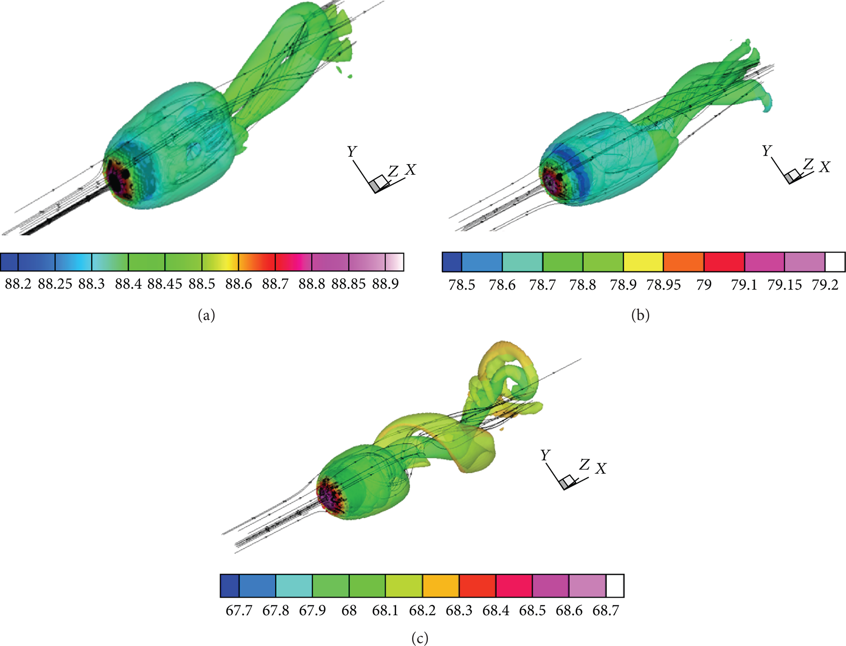
Comparison of sound source distribution around rotating ellipsoids (τ = 125).

Visualizations of flows are shown in Figures 6 and 7. In Figure 6, the λ2 method which was proposed by Jeong and Hussain [13] is used for the visualization of vortical structure. The λ2 method can extract the domain where the local pressure is minimum, which eliminated incorrect recognition of the vortex caused by unsteady condition and viscous force, and can capture a core of vortex exactly. The color indicates pressure and the figure has the streamline in addition. For the flow around the nonrotating sphere, hairpin-like vortical structure is observed. There is a close resemblance between the present result and the experiment which was carried out by Sakamoto and Haniu [14]. For the flow in the condition where the sphere is rotating, it is observed that the vortex itself which is transported to the region behind the object is rotated. The hairpin-like vortex changed to a spiral complicated one. In Re_r = 1000, the rotation effect is predominant, and it turns out that the hairpin-like vortex moves in a spiral way.

Figure 7 visualizes the Powell sound source in slices of Y = 3D and Z = 3D. The sound source is generated near the object, and many sound sources also occurred from the wake at the high Reynolds number. Besides, it is turned out that there is less generation of a sound source around the ellipsoid compared with the sphere under the same Reynolds number. Also at Re = 500, if there is a rotation of an object, it is recognized from Figure 7 that the sound source of a quantity equivalent to or more than that of Re = 1000, Re_r = 0 (nonrotation) is generated. At Re = 500, Re_r = 1000, by the great influence of rotation, generation of the sound source in a wake is remarkable, and it is carried to a distant position. Furthermore, it is observed that generation of the sound source in the wake is also promoted in Re = 1000 and Re_r = 500 condition in which external uniform flow is predominant.

7. Computation around Flapping Ellipsoid

7.1. Analysis Conditions

The level set IB method allows us to conduct moving boundary computations with sufficient accuracy of tracking borders without excessive calculation load. In this section, as an example of analysis of the moving boundary by the IB method, flow analysis around the oscillating ellipsoid which imitates flapping wings is conducted. Here, some typical values are given based on flying insects.

An analysis model is shown in Figure 8. A computational area is taken as shown in Figure 8. A flat ellipsoid is installed in the center, and it performs a periodic up-and-down motion. In this ellipsoid, the long radius of the Y – Z section is D, and the short diameter is 0.2D, and another diameter of the X – Z section is also 0.2D. It is assumed that an external uniform flow along x-axis direction in the whole domain is given, and nondimensional angular velocity is given between 45 degrees of flapping angle. The ellipsoid is shuttling between 22.5 and −22.5 degrees, and the ellipsoid is not twisted in the direction of x-axis. The Reynolds number of an external uniform flow is set to Re = 167, and that of a flapping of wings is set to Re_r = 350. This analysis assumes plane symmetry with respect to the center plane (Y = 0), and thus it makes V = 0 at the plane; the Neumann type boundary condition is used for other velocity components and the pressure at a side wall and the upper and lower walls. The number of grids is (X, Y, Z) = (96, 80,132), a calculation area is 4D × 3D × 8D, and the center position of the object is (2D, 0, 4D). Moreover, relating to the movement of the object, position information is obtained from the velocity of the object, and the position of the object is overwritten for every time step.

Figure 8:

Schematic model of the flapping ellipsoids.

7.2. Results and Discussion

First, from Figure 9, it exhibits that the lift force is changing periodically caused by the flapping of the object. It turns out that the flow is calculated along the object boundary with sufficient accuracy even when a boundary changes for every time. Figure 10 shows the vortical structure by the λ2 method, and Figure 11 shows the distribution of sound source on the slice with respect to X = 2D and Y = 0. Also, from Figures 10 and 11, it turns out that vortical structure and a sound source change periodically, and they have changed to the complicated flow in a wake. It can be observed that the vortical structure and the sound source which were generated by the flapping wings are convected by the external uniform flow. And it is especially observed that the sound source is generated in the back of the object and also near the wingtip where the angular velocity takes its maximum. Moreover, it turns out that the sound source is generated at a nearly constant period around the whole object and in the wake which is separated from the object.

Figure 9:

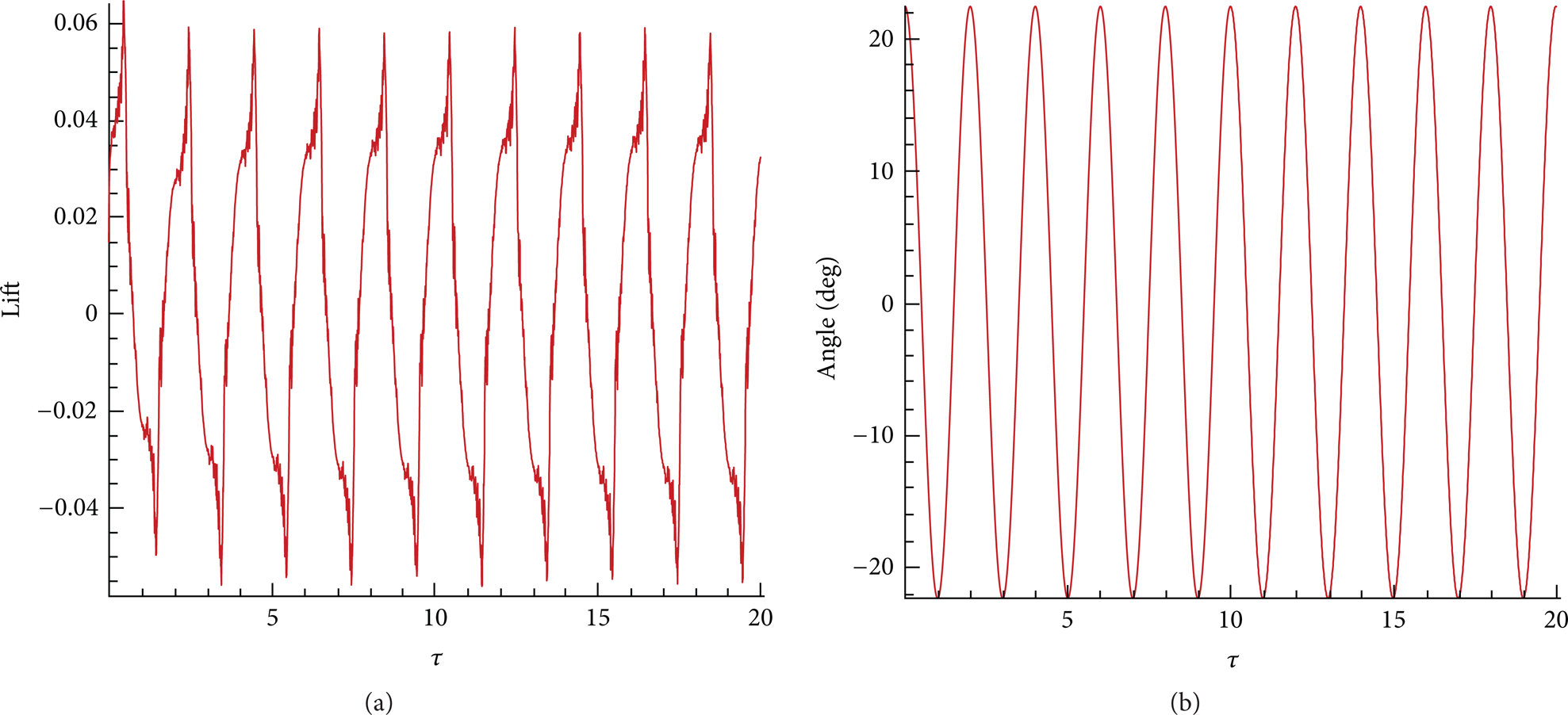
The graph of τ-lift (left) and τ-angle (right).

Figure 10:

Vortical structure around flapping ellipsoids (τ = 17) (a) 3D angle, (b) X – Z slice.

Figure 11:

Sound source distribution around a flapping ellipsoid (τ = 17).

8. Computation around a Rotating Ellipsoid

8.1. Computational Conditions

Finally, flow computation around the object which imitates the windmill of two-wings is conducted. The initial condition and the boundary condition are set up like the computation around a rotating sphere and an ellipsoid. Figure 12 shows an analysis model. A computational area is shown in Figure 12. An ellipsoid is installed in the center, and it rotates with a constant angular velocity. The ellipsoid has the long radius of D and the short diameter of 0.2D in the Y – Z slice, and the short diameter of 0.067D in the X – Z slice. It is assumed that a uniform flow in the whole domain is given, and the rotation starts with nondimension angular velocity Ω = Re_r/Re from the position whose angle with the X – Y slice is 90 degrees. The number of grids is (X, Y, Z) = (170,140,140), a calculation area is 4D × 4D × 4D, and the center position of the object is (D, 2D, 2D). The regular Reynolds number of external uniform flow is Re = 500, and the Reynolds number which results from rotation is Re_r = 500.

Figure 12:

Schematic model of the rotating ellipsoid.

Moreover, as having shown in the analysis of the moving boundary which imitates flapping wings in the preceding section, relating to the movement of the object, position information is obtained from the velocity of the object, and the position of the object is overwritten for every time step.

8.2. Results and Discussion

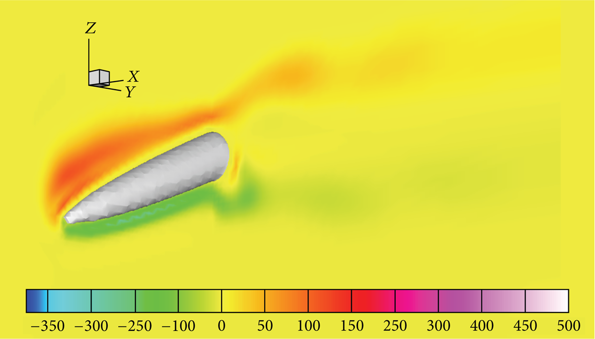
Figure 13 shows a vortical structure by the IB method for the flow imitating the windmill, and Figure 14 shows the distribution of the Powell sound source at the slices of (a) X = D and Y = 2D, (b) Z = 2D, (c) Y = 2D, and (d) X = 1.3D, respectively. From Figure 13, the vortex which occurred by rotation is convected backward by the external uniform flow without breaking off, and it can be observed that the flow has changed to the complicated flow in the wake. This shows that the level set IB method can trace and calculate the flow around the moving boundary with sufficient accuracy. Especially it is recognized from Figure 14 that the sound source has occurred near the object, the wake, and the wingtip. Besides, in each slice of figures, the sound source in the wake behaves like the Karman's vortices and occurs far away compared with the case of the flapping wings.

Figure 13:

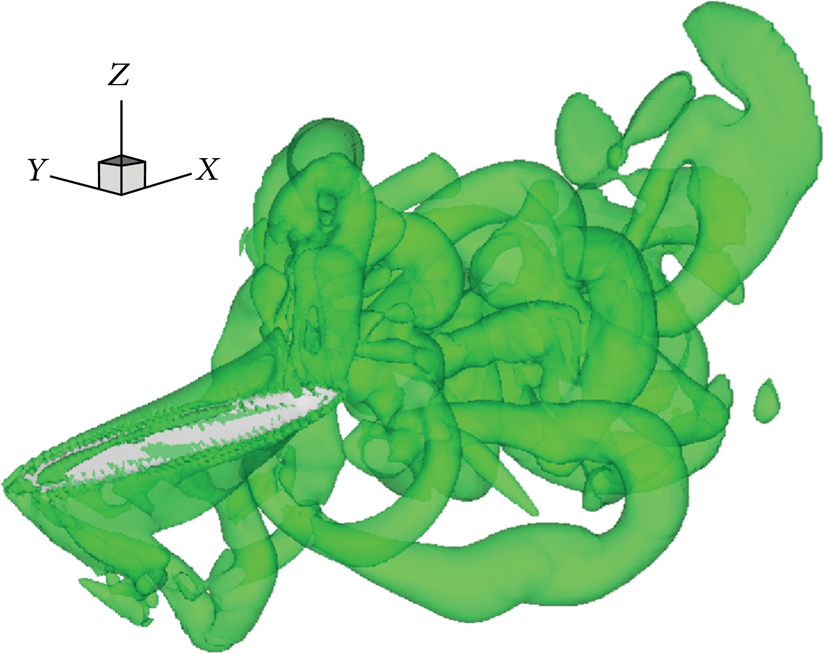
Vortical structure of a rotating ellipsoid (τ = 20).

Figure 14:

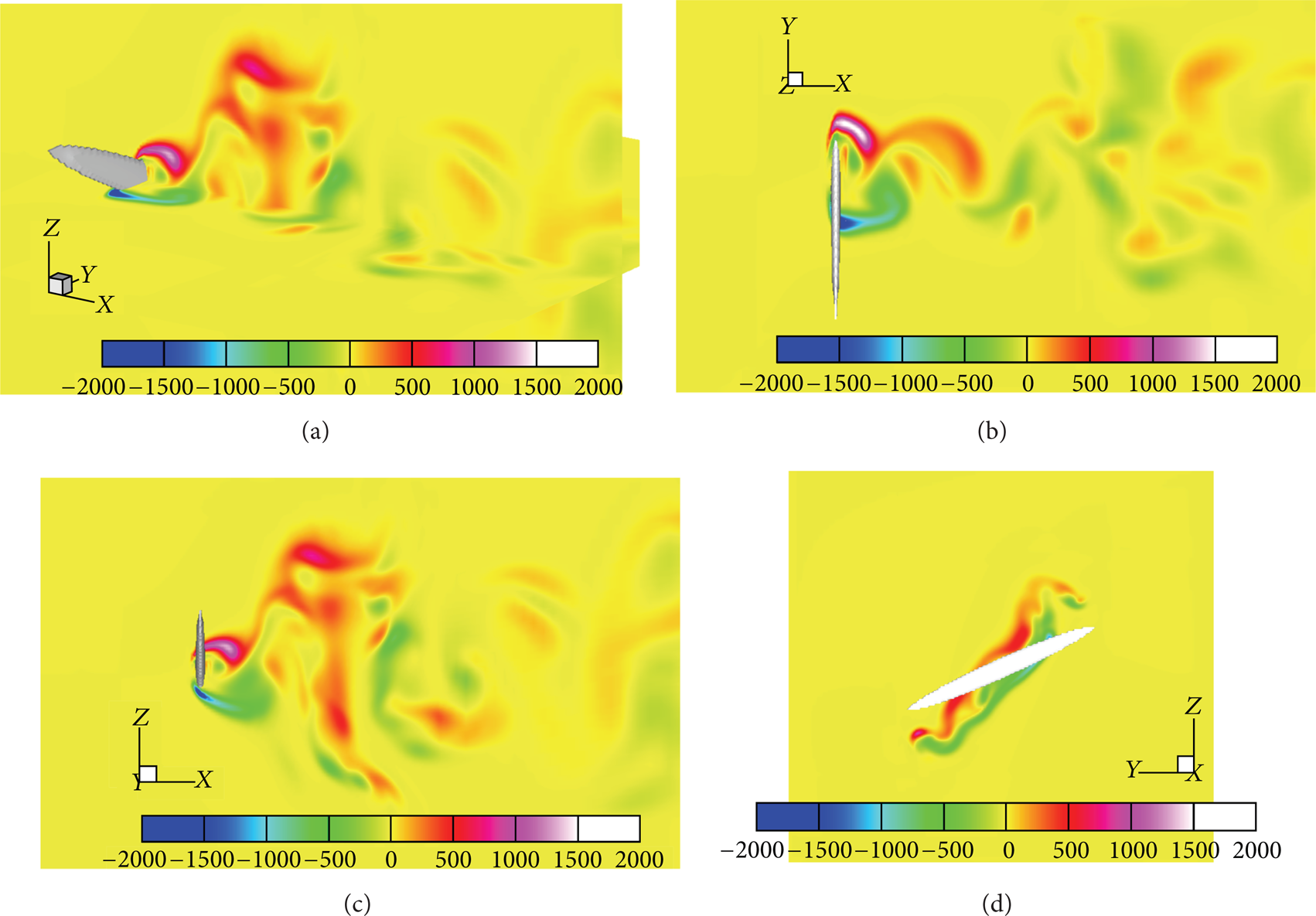
Sound source distribution around rotating ellipsoids (τ = 20). (a) 3D angle, (b) X – Y slice, (c) X – Z slice, and (d) Y – Z slice.

9. Conclusion

In this study, we computed several typical flows around stationary, rotating, or moving objects by using the level set IB method. It combines the advantages of level set method and IB method in order to be able to capture the shape of object accurately. Also we visualized the vortical structure and obtained the generating mechanism of the sound source.

By this research, the boundary of a moving object is able to be traced with sufficient accuracy. Moreover, the coefficients of drag and lift were obtained for various types of object that is stationary, rotating, or moving in the wide range of the Reynolds number. The code also can visualize the vortical structure and sound source distribution for various conditions, so it can be considered that these are highly useful and innovative.

Footnotes

Nomenclature

References

Peskin

C. S.

, “Flow patterns around heart valves: a numerical method,” Journal of Computational Physics, vol. 10, no. 2, pp. 252–271, 1972.

Okita

Tawara

, and Ono

, “Development of CFD techniques based on VCAD data,” in RIKEN Symposium, March 2008.

Sato

, Numerical analysis of incompressible flows by an Immersed Boundary Method with the Level Set Method [M.S. thesis], Tokyo Metropolitan University, 2010.

Lighthill

M. J.

, “On sound generated aerodynamically. Part I: General theory,” Proceedings of the Royal Society A, vol. 221, no. 1107, pp. 564–587, 1952.

Powell

, “Theory of vortex sound,” Journal of the Acoustical Society of America, vol. 36, pp. 177–195, 1964.

Yoshida

Watanabe

, and Nakamura

, “Numerical study of outflow boundary conditions for time-dependent incompressible flows,” Transactions of the Japan Society of Mechanical Engineers B, vol. 61, no. 588, pp. 2887–2895, 1995.

Mittal

, “A fourier-chebyshev spectral collocation method for simulating flow past spheres and spheroids,” International Journal for Numerical Methods in Fluids, vol. 30, no. 7, pp. 921–937, 1999.

Gilmanov

Sotiropoulos

, and Balaras

, “A general reconstruction algorithm for simulating flows with complex 3D immersed boundaries on Cartersian grids,” Journal of Computational Physics, vol. 191, no. 2, pp. 660–669, 2003.

10.

Campregher

Militzer

Mansur

S. S.

, and Da Silveira Neto

, “Computations of the flow past a still sphere at moderate reynolds numbers using an immersed boundary method,” Journal of the Brazilian Society of Mechanical Sciences and Engineering, vol. 31, no. 4, pp. 344–352, 2009.

11.

Jones

D. A.

and Clarke

D. B.

, “Simulation of flow past a sphere using the fluent code,” DSTO Document, 2008.

12.

Poon

Iaccarino

Andrew

, and Giacobello

, “Numerical studies of high Reynolds number flow past a stationary and rotating sphere,” in Proceedings of the 7th International Conference on CFD in the Minerals and Process Industries, Melbourne, Australia, 2009.

13.

Jeong

and Hussain

, “On the identification of a vortex,” Journal of Fluid Mechanics, vol. 285, pp. 69–94, 1995.

14.

Sakamoto

and Haniu

, “A study on vortex shedding from spheres in a uniform flow,” Journal of Fluids Engineering, vol. 112, no. 4, pp. 386–392, 1990.