Sage Journals: Discover world-class research

Abstract

The design and analysis of routing algorithm is an important issue in wireless sensor networks (WSNs). Most traditional geographical routing algorithms cannot achieve good performance in duty-cycled networks. In this paper, we propose a k-connected overlapping clustering approach with energy awareness, namely, k-OCHE, for routing in WSNs. The basic idea of this approach is to select a cluster head by energy availability (EA) status. The k-OCHE scheme adopts a sleep scheduling strategy of CKN, where neighbors will remain awake to keep it k connected, so that it can balance energy distributions well. Compared with traditional routing algorithms, the proposed k-OCHE approach obtains a balanced load distribution, consequently a longer network lifetime, and a quicker routing recovery time.

1. Introduction

Studying the behavior of dynamic sensor networks becomes a hot topic. Movements of nodes make the wireless sensor networks (WSNs) [1] a dynamic one. These nodes can communicate with each other in wireless communication radius without any static network interactions. An important issue in dynamic geographical networks is the design and analysis of routing algorithms. Due to the limited communication range of the wireless transceivers, mobile nodes cannot communicate with other nodes unless they are within each other's geographical regions [2, 3]. Thus, it may be necessary for a mobile node to require aids of other nodes after checking their geographical routing information in forwarding data packets to its destination.

It will be much more uncertain when we consider the routing issue in a duty-cycled network, since the duty-cycle scheduling aims to prolong the network lifetime [4, 5] by making some nodes sleep and wake up when packets transmission occurs. Studies on adopting conventional routing protocols in wireless sensor network in a dynamic convention have been generally discussed [3, 6]. Our interest in the routing problem in a duty-cycled network falls into the following two aspects: (1) existing routing algorithm could place a heavy load on a newly joined node due to routing table updates and (2) the wireless network connectivity.

Conventional routing algorithms concentrate on finding the shortest path, without much concern about critical issues such as energy efficiency and network lifetime. The problem we discuss here is how to route efficiently in a duty-cycled sensor network. The basic idea behind the algorithms is to divide the network into a number of overlapping clusters. A node's sleep scheduling leads to a change in the network topology, then the membership of cluster changes as well. We propose a cluster formation scheme called k-OCHE, which selects cluster heads considering energy availability firstly, and then the cluster heads recruit cluster members. This cluster creation scheme can well be adopted in different routing circumstances.

The rest of this paper is organized as follows. Section 2, we survey related work. Section 3 defines network model, sleeping scheduling model, energy consumption model, and some notations. In Sections 4 and 5, we further detail the k-OCHE scheme and routing algorithm. We present specifics of simulation experiments which validate the correctness of the proposed algorithm in Section 6. Finally, Section 7 concludes the paper.

2. Related Work

Similar to other networks, overload balance, prolonging lifetime, and scalability are the major design concerns of wireless sensor networks. In conventional multihop communications in WSNs, sensors close to the sink are often overloaded, resulting in increased latency and reduced network life span. Such overload might cause latency in communication and reduce life span of network. In addition, the original architecture is not scalable for larger set of sensors covering a wider area of interest. To allow the network to cope with additional load and to be able to afford a large area of interest, clustering routing has been pursued. The main aim of clustering routing is to efficiently maintain the energy consumption of sensor nodes by involving them in multihop communication with a particular cluster and by performing data aggregation and fusion to reduce the number of transmitted messages to sink.

2.1. Routing Protocols

Many routing protocols [7–11] have been studied in the field of wireless sensor networks. Karp and Kung present greedy perimeter stateless routing (GPSR) [7], a novel routing protocol for wireless datagram networks that uses the positions of routers and a packet's destination to make packet forwarding decisions. GPSR makes greedy forwarding decisions using only information about a router's immediate neighbors in the network topology. When a packet reaches a region where greedy forwarding is impossible, the algorithm recovers by routing around the perimeter of the region. By keeping state only about the local topology, GPSR scales better in perrouter state than shortest-path and ad-hoc routing protocols as the number of network destinations increases. Under mobility's frequent topology changes, GPSR can use local topology information to find correct new routes quickly.

Shu et al. propose an efficient two-phase geographic greedy forwarding (TPGF) [8] routing algorithm for WMSNs. TPGF takes into account both the requirements of real-time multimedia transmission and the realistic characteristics of WMSNs. It finds one shortest (near shortest) path per execution and can be executed repeatedly to find more on-demand shortest (near shortest) node-disjoint routing paths. TPGF supports three features: (1) hole bypassing, (2) the shortest path transmission, and (3) multipath transmission, at the same time. TPGF is a pure geographic greedy forwarding routing algorithm, which does not include the face routing, for example, right/left hand rules and does not use planarization algorithms, for example, GG or RNG. This point allows more links to be available for TPGF to explore more routing paths and enables TPGF to be different from many existing geographic routing algorithms.

However, these traditional routing algorithm will overload relay nodes with the increase in sensor density. Besides, convergence characteristics of these algorithm are not good enough to meet the need of dynamic networks, such as duty-cycled networks.

2.2. Cluster-Based Approach for Routing

In the last few years, many algorithms have been proposed for clustering routing in wireless sensor networks [12–24].

In [14], Heinzelman et al. have proposed a distributed algorithm for wireless sensor networks (LEACH) in which sensors randomly select themselves as cluster heads with some probability and broadcast their decisions. The remaining sensors join the cluster of the cluster head that requires minimum communication energy. LEACH is one of the most popular clustering routing algorithms for sensor networks and is completely distributed. However, LEACH uses single-hop routing where each node can transmit directly to the cluster head and the sink. Besides, there are a number of clustering algorithms constructing clusters not more than 1-hop away from a cluster head, such as DCA [15] and DMAC [17]. Similar to these, Baker and Ephremides [13] propose overlapping cluster with $k = 1$ . In large networks single-hop clustering, as shown in Figure 2, may generate a large number of cluster heads and eventually lead to the same problems as if there is no clustering.

In addition, the TEEN [16] and APTEEN [18] are hierarchical protocols designed to be responsive to sudden changes in the sensed attributes such as temperature. Younis et al. [19] have proposed a different hierarchical routing algorithm based on a threetier architecture.

To the best of our knowledge, there is only one clustering algorithm that specifically controls overlapping in the formation of clusters, that is, KOCA [20]. Goal of KOCA is to ensure that the entire network is covered with connected overlapping clusters considering a specific average overlapping degree. KOCA is still a static clustering in which the cluster formation is not changed all the time. This condition causes an unbalance load among all nodes. A node that roles as cluster head (CH) will get more load than a non-CH and so that it will die faster. The death of CHs will break the whole network because the link between nodes and center will be broken. Therefore, KOCA cannot be applied in actual situation commendably. Rotating the CH role distributes this higher burden among the nodes, thereby preventing the CH from dying prematurely. To overcome this problem, we propose k-OCHE which allows a node to go to sleep while keeping its neighbors k connected, thus the role of CH can be rotated and the load of CH can be balanced. The most important is that k-OCHE is the first approach to combine the interior cluster routing with exterior cluster routing which achieves balanced load distribution, longer network lifetime, and quicker routing.

3. Assumptions and Notations

3.1. Network Model

We consider a multihop wireless sensor network where all nodes are alike. We assume that each node has a unique id. The locations of sensor nodes can be obtained by GPS. All sensors transmit at the same power level and hence have the same transmission range $T_{r}$ . Each sensor node is aware of its geographic location and its 1-hop neighbor nodes' geographic locations. We assume that sensor nodes can know the location of base station by receiving the packet, which comes from there. This assumption is the same as that used in [7, 25, 26].

All communications are over a single shared wireless channel. A wireless link can be established between a pair of nodes only if they are within wireless range of each other. The k-OCHE algorithm only considers bidirectional links. It is assumed that MAC layer will mask unidirectional links and pass bidirectional links to k-OCHE. We refer to any two nodes that have a wireless link as 1-hop or immediate neighbors. Nodes can identify neighbors using beacons.

3.2. Sleeping Scheduling Model

To ensure the network connectivity and prolong its lifetime, we assume that all nodes operate under CKN-based [27] sleep/awake duty cycling. Time is divided into epochs, and each epoch is T. On each epoch, nodes run CKN, shown in Algorithm 2, to decide whether to be awake. A node can go to sleep assuming that at least k of its neighbors remain awake to keep it k connected. And nodes reach a consensus to take turns to sleep, while the whole network is globally connected. Therefore, by changing the value of k, the network can manipulate the sleep rate s, so that it can proceed with further work with clustering.

3.3. Energy Consumption Model

We use the same radio model defined in [28]. The amount of energy required to transmit an L-bit message over a distance x is $E_{TX} (L, x)$ given by (1)

\begin{matrix} E_{TX} (L, x) = {\begin{cases} E_{elec} \cdot L + ϵ_{f s} \cdot L \cdot x^{2}, & if x \leq d_{0}, \\ E_{elec} \cdot L + ϵ_{m p} \cdot L \cdot x^{4}, & if x \geq d_{0} . \end{cases} \end{matrix}

(1)

$E_{elec}$ is the energy dissipating to power the transmitter or receiver circuitry. The parameters $ϵ_{f s}$ and $ϵ_{m p}$ are the amount of energy dissipating per bit in the radio frequency amplifier according to the distance $d_{0}$ , which is given by (2)

\begin{matrix} d_{0} = \sqrt{\frac{ϵ_{f s}}{ϵ_{m p}}} . \end{matrix}

(2)

The energy consumed by receiving this packet is $E_{TX} (L, x)$ shown by (3),

\begin{matrix} E_{TX} (L, x) = L \cdot E_{elec} . \end{matrix}

(3)

3.4. Notations

(1) Network size (n): the number of nodes in the network. Sensor nodes are deployed randomly in a square area with side length of l.

(2) Energy consumption rate (EC): for each node, $E R_{i}$ denotes residual energy on the battery, and then EC can be defined as (4),

\begin{matrix} EC = \frac{E R_{i}}{E_{initial}}, \end{matrix}

(4)

where

E_{initial}

is the initial energy of each node.

(3) Energy availability (EA):

\begin{matrix} E A_{i} = E_{initial} - EC * t . \end{matrix}

(5)

(4) Minimum number of awake neighbors in an epoch for each node (k): through varying the value of k, we can keep the network k connected and optimize the geographic routing performance.

(5) Average node degree (d): the average degree of a node u is the number of its neighbor nodes. The relation between the average node degree (d) and the radio range (r) of a node is given by

\begin{matrix} d = \frac{n π r^{2}}{l^{2}} = μ π r^{2} . \end{matrix}

(6)

4. The k-OCHE Algorithm

4.1. The Proposed Algorithm

In k-OCHE, shown in Algorithm 1, a node can go to sleep assuming that at least k of its neighbors remain awake to keep it k connected. Given a k, we can obtain a new network topology within the range of awake nodes in each cycle. Each node can have three possible states: cluster heads (CHs), boundary nodes (BNs), and normal nodes. A cluster head possesses information about not only its own cluster (such as member nodes' IDs) but also adjacent clusters (such as boundary node and adjacent clusters' members). A boundary node belongs to multiple overlapping clusters connecting different clusters to transfer and forward data, and it improves the network robustness effectively. Normal nodes are internal nodes that belong only to one cluster.

Algorithm 1: The k-OCHE algorithm.

(*Run the following at each node u*)

(1) Get the information of current remaining energy EA.

(2) Set $C H_t a b l e_w a i t$ timer;

(3) if $E A \geq T h r e s h o l d$ then

(4) status = CH;

(5) Broadcast $C H_A D$ containing (CHID, CHEA, HC, SEA) to neighbors.

(6) if Receive a $C H_A D$ then

(7) If $C H_A D . C H E A > E A$ then

(8) status = NORMAL;

(9) end if

(10) end if

(11) Receive $J_A D$ from neighbors.

(12) if $C H_t a b l e$ does not contains $J_A D$ .NID then

(13) Add $J_A D$ .NID to $C H_t a b l e$ ;

(14) $C H_t a b l e_w a i t$ timer fires;

(15) Broadcast $C H_t a b l e$ to its members.

(16) end if

(17) else

(18) status = NORMAL;

(19) Receive a message.

(20) if $t i m e r \geq H A L F_O F_C K N_C Y C L E$ then

(21) status = CH;

(22) end if

(23) if message == $C H_A D$ from CH(s) then

(24) Add $C H_A D$ .CHID to $C H_t a b l e$ ;

(25) $C H_t a b l e . P I D$ = $C H_A D$ .SID;

(26) $C H_t a b l e_w a i t$ timer fires;

(27) Send $J_A D$ to its parent node.

(28) if $C H_A D . H C < n$ then

(29) HC=HC+1;

(30) Broadcast $C H_A D$ to neighbors.

(31) end if

(32) else

(33) if message == $J_A D$ then

(34) Send the $J_A D$ to its parent node.

(35) else

(36) if message == $C H_t a b l e$ from CH(s) then

(37) Update its $C H_t a b l e$ .

(38) end if

(39) end if

(40) end if

(41) if its $C H_t a b l e$ has more than one CHID then

(42) Status = Boundary;

(43) Add $C H_t a b l e$ .CHID to $N C H_t a b l e$ ;

(44) Send its $C H_t a b l e$ and $N C H_t a b l e$ to its parent node.

(45) else

(46) Receive $C H_t a b l e$ and $N C H_t a b l e$ from Boundary nodes.

(47) end if

(48) end if

Algorithm 2: Connected K neighborhood (CKN).

(*For each node $u^{*}$ )

(1) Pick a random rank ${r a n k}_{u}$ .

(2) Broadcast ${r a n k}_{u}$ and receive the ranks of its currently awake neighbors $N_{u}$ . Let $R_{u}$ be the set of these ranks.

(3) Broadcast $R_{u}$ and receive $R_{v}$ from each $v \in N_{u}$ .

(4) If $| N_{u} |$ < k or $| N_{v} |$ < k for any $v \in N_{u}$ , remain awake.

Return.

(5) Compute $C_{u} = {v | v \in N_{u}$ and ${r a n k}_{v} > {r a n k}_{u}}$ ;

(6) Go to sleep if both the following conditions hold. Remain awake otherwise.

(i) Any two nodes in $C_{u}$ are connected either directly themselves or indirectly through nodes within u's

2-hop neighbors that have $r a n k$ larger than E $r a n k_{u}$ ;

(ii) Any node in $N_{u}$ has at least k neighbors from $C_{u}$ .

(7) Return.

In this section, we present the description of the cluster head's selection process as well as the clusters' generation; we then give an example to illustrate a cluster generated by k-OCHE.

4.2. Cluster Head Selection Procedure

In k-OCHE approach, the important operation is to select a set of cluster heads (CHs) among the nodes in the network and recruit the normal nodes as these CHs' members. The k-OCHE approach adopts EA to select CHs, and EA is defined as the battery residual energy after certain consumption during a certain period. At the beginning of each cycle, each node compares its EA to the threshold (the threshold is an empirical value, which is used to control the number of CHs in the network. The optimal threshold is obtained when the CH nodes take $15 %$ [20] of all the nodes in the network. And we use this value for experiments presented in this paper.), if its EA is bigger than the threshold, then it becomes a CH and advertises itself as a CH to the sensors within its transmission range to recruit cluster members. This advertisement ( $C H_A D$ ) is forwarded to all sensors that are no more than n hops away from the CH through controlled flooding. The recruitment message's ( $C H_A D$ ) header includes CHID, SID, EA, and HC, where CHID is cluster head ID, SID is the sender node ID, and HC is the number of hops leading to the CH node. The HC field is used to limit the flooding of the $C H_A D$ message to n hops. By receiving the recruit message from CHs, a sensor node joins those clusters no matter whether it has belonged to a cluster.

However, if a CH u receives a recruit from another CH v, and v has the higher EA, then u gives up being a CH and joins v's cluster. Since the $C H_A D$ forwarding is limited to n hops, if a sensor does not receive a CH advertisement within a reasonable time duration, it can infer that it is not within n hops of any cluster head and hence become a CH. In k-OCHE, the maximum time that a node should wait for CH advertisement message is set to half cycle of CKN. Note that this is a distributed algorithm and does not demand clock synchronization between the sensors.

4.3. Cluster Generation

Each node maintains a table, $C H_t a b l e$ , that stores information about the clusters it belongs to. Upon receiving a new $C H_A D$ message, a node will add an entry in its $C H_t a b l e$ and check the HC field in the message. Then the node updates HC and parent fields in the corresponding entry in the CH table if the recent message came over a shorter path. Often a message traveling the shortest path in terms of the number of hops would arrive first. However, delay may be suffered at the MAC or link layers. For every entry in its $C H_t a b l e$ , a node sends a join advertisement ( $J_A D$ ) message to CH in order to become a member of the corresponding cluster. To limit the flooding, the $J_A D$ message is unicasted using the field $C H_t a b l e . p a r e n t$ . The $J_A D$ message has the form [SID, CHID, EA] where SID is the ID of the node that will join the cluster and CHID is the ID of the CH node responsible for this cluster. Upon receiving the $J_A D$ message, the parent node will add SID to its children field. When a CH node receives join advertisement ( $J_A D$ ) sent by an ordinary node, it will compare the number of member nodes to threshold to admit new member and update the count of cluster nodes if the size is smaller than threshold or else abandon the request. Supposing that the rejected node has cluster head already, the clustering process ceases. Otherwise, it looks for another appropriate cluster to join in. There is only one single CHID entry in a ordinary node's CH table, because it belongs to one cluster head, while the overlapping cluster node which connects different clusters has multiple CHID entries. Each cluster head maintains a list of all cluster members, a list of adjacent clusters, and a list of boundary nodes.

The k-OCHE algorithm avoids the fixed cluster head scheme, with periodic replacement done by sleep scheduling mechanism to balance the node energy consumption. All cluster members send the current state information to cluster head, and k-OCHE chooses the node with the highest EA to be the new head. When the new cluster head gets cluster head's notification, it broadcasts recruitment message and the new cluster forming phase triggers. The process can reduce the energy consumption of broadcast of temporary head.

Note that k-OCHE stops in $O (n)$ steps. As n is a constant value, the clustering process terminates in a constant number of iterations regardless of the network size.

4.4. An Illustrative Example

We demonstrate our algorithm with Figure 1, which is selected from the simulation results optionally, and we add some necessary information to make it more comprehensible.

Figure 1

An example of overlapping clusters in a network with 38 nodes. After executing k-OCHE, the network selects three cluster heads, and each cluster contains 9 normal nodes. Clusters can communicate with each other through boundary nodes.

Figure 2

Single hop clustering. Each node in the network is not more than 1-hop away from a cluster head.

In Figure 1, there are three clusters with three corresponding cluster heads A, B, and C, and nodes with black frame in the overlapping area are boundary nodes. Note that two cluster heads are not immediate neighbors. Since boundary nodes belong to multiple clusters, their tables contain CHs of those clusters. A, B, and C can communicate with each other through their common boundary nodes in their neighbor cluster head tables.

5. Routing Algorithm

We first discuss the necessary data structures to be maintained at each node for the routing algorithm, as shown in Table 7. We then explain the routing construction and recovery procedures in the network. The routing construction can be divided into two phases: interior cluster routing and exterior cluster routing.

During the interior and exterior routing phase, routes are constructed between all pairs of nodes. The routing recovery phase takes care of maintaining routing table considering sleep schedule and recovering from an individual node failure.

5.1. Interior Cluster Routing

After cluster head selection and cluster generation procedure, each node completes the construction of two tables: $C H_t a b l e$ and $N C H_t a b l e$ . $C H_t a b l e$ stores the information of cluster it belongs to and $N C H_t a b l e$ stores the information of its neighbor clusters. In interior cluster routing construction phase, each node constructs interior cluster routing table according to $C H_t a b l e$ and $N C H_t a b l e$ . At each node u, (i)

when $r o u t i n g_t a b l e . D e s$ is u's child or grandchild, u updates $r o u t i n g_t a b l e . n e x t$ by using $C H_t a b l e . C R I D$ ,

(ii)

when $r o u t i n g_t a b l e . D e s$ is in the same cluster with u, u updates $r o u t i n g_t a b l e . n e x t$ by using $C H_t a b l e . P I D$ ,

(iii)

when $r o u t i n g_t a b l e . D e s$ is in neighbor cluster, u updates $r o u t i n g_t a b l e . n e x t$ by using $N C H_t a b l e . R I D$ ,

(iv)

when $r o u t i n g_t a b l e . D e s$ is one of the others, u updates $r o u t i n g_t a b l e . n e x t$ by using $C H_t a b l e . P I D$ .

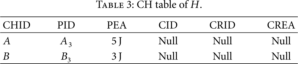
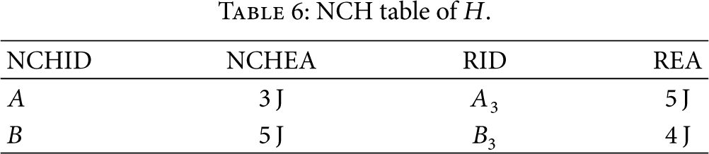
Let us illustrate it with an example. Tables 1, 2, 3, 4, 5, and 6 are $C H_t a b l e s$ and $N C H_t a b l e s$ of A, $A_{3}$ , and H. For cluster A, we take the CH node A, a normal node $A_{3}$ , and a boundary node H into consideration. As the structure of cluster is a spanning tree, the root is A, level-1 children are $A_{1}$ , $A_{2}$ , $A_{3}$ , $A_{4}$ , and F, and level-2 children are $A_{5}$ , $A_{6}$ , H, and G.

Table 1

CH table of A.

CHID	PID	PEA	CID	CRID	CREA
			$A_{1}$ , $A_{2}$ , $A_{3}$	$A_{1}$ , $A_{2}$ , $A_{3}$	5 J, 4 J, 4 J
A	Null	Null	$A_{4}$ , $A_{5}$ , $A_{6}$	$A_{4}$ , $A_{1}$ , $A_{1}$	3 J, 4 J, 5 J
			F, G, H	F, $A_{3}$ , $A_{3}$	5 J, 3 J, 4 J

Table 2

CH table of $A_{3}$ .

CHID	PID	PEA	CID	CRID	CREA
A	A	5 J	G, H	G, H	4 J, 5 J

Table 3

CH table of H.

CHID	PID	PEA	CID	CRID	CREA
A	$A_{3}$	5 J	Null	Null	Null
B	$B_{3}$	3 J	Null	Null	Null

Table 4

NCH table of A.

NCHID	NCHEA	RID	REA
B	4 J	$A_{3}$	4 J
C	5 J	$A_{3}$ , F	3 J, 5 J

Table 5

NCH table of $A_{3}$ .

NCHID	NCHEA	RID	REA
B	3 J	H, G	4 J, 3 J
C	4 J	G	5 J

Table 6

NCH table of H.

NCHID	NCHEA	RID	REA
A	3 J	$A_{3}$	5 J
B	5 J	$B_{3}$	4 J

Table 7

Data structures table.

Data structures	Description
CH_AD (CHID, CHEA, HC, SEA)	A message containing CHID (the ID of cluster head), CHEA (the energy availability of cluster head), HC (hop count), and SEA (the energy availability of message sender)
J_AD (ID, SEA)	A message containing ID (the ID of join node), SEA (the energy availability of message sender)
B_AD (NCHID)	A message containing NCHID (the ID of neighbor cluster head)
CH_table (CHID, PID, PEA, CID, CRID, CREA)	A table containing CHID (the ID of cluster head), PID (the ID of parent node), PEA (the energy availability of parent node), CID (the ID of its children node), CRID (the ID of children's relay node), and CREA (the energy availability of children's relay node)
NCH_table (NCHID, RID, REA)	A table containing NCHID (the ID of neighbor cluster head), RID (the ID of neighbor cluster head's relay node), and REA (the energy availability of neighbor cluster head's relay node)
Routing_table (destination, next hop)	A routing table containing destination and next hop

In the routing table of A, when destinations are $A_{1}$ to $A_{6}$ , F, G, and H, A will check $C H_t a b l e . C R I D$ to choose the next hop, as they are all its level-1 or level-2 children. When destinations are $B . *$ and $C . *$ , A will check $N C H_t a b l e . R I D$ to choose the next hop, as they are in neighbor clusters. For the other destinations, A uses exterior cluster routing which will be discussed in the following section.

In the routing table of $A_{3}$ , when destinations are G and H, $A_{3}$ will check $C H_t a b l e . C R I D$ to choose the next hop, as they are its children. When destinations are $B . *$ and $C . *$ , $A_{3}$ will check $N C H_t a b l e . R I D$ to choose the next hop, as they are in neighbor clusters. Considering that $C H_t a b l e . C R I D$ has two nodes, G and H, $A_{3}$ will choose the node of higher EA to be the next hop. For the other destinations, $A_{3}$ will check $C H_t a b l e . P I D$ to choose the next hop.

In the routing table of H, when destinations are in neighbor cluster, H will check $N C H_t a b l e . R I D$ to choose the next hop, as they are in neighbor clusters. For the other destinations, H will check $C H_t a b l e . P I D$ to choose the next hop. Considering that $C H_t a b l e . P I D$ has two entries, H will choose the node of higher EA to be the next hop. The results of routing table of A, $A_{3}$ , and H are shown in Tables 8, 9, and 10.

Table 8

Routing table of A.

Destination	Next hop
$A . A_{1} \dots A$ . $A_{6}$	$A_{1}$ , $A_{2}$ , $A_{3}$ , $A_{4}$ , $A_{1}$ , $A_{1}$
A.F	F
A.G	$A_{3}$
A.H	$A_{3}$
B.*	$A_{3}$
C.*	$A_{3}$ /F (higher EA)
.	Outer Routing

Table 9

Routing table of $A_{3}$ .

Destination	Next hop
$A . G$	G
A.H	H
B.*	H/G (higher EA)
C.*	G
.	A

Table 10

Routing table of H.

Destination	Next hop
A.*	$A_{3}$
B.*	$B_{3}$
.	$A_{3}$ / $B_{3}$ (higher EA)

5.2. Exterior Cluster Routing Construction

We consider each cluster as a node in exterior cluster routing phase. Each CH node takes the responsibility of each cluster. An original routing algorithm (e.g., GPSR and TPGF algorithms) is running exterior clusters. As shown in Figure 3, each hexagon presents a cluster and the black nodes are CH nodes. The normal nodes are ignored except source and sink. When source node s sends a packet to sink node d, s node will run interior cluster routing and then packet will be relayed to CH node A. At that time, A will run exterior cluster routing to decide which neighbor cluster to be the relay cluster and then run interior cluster routing to the CH node of relay cluster. In general, as shown in Figure 3, the routing path of GPSR is straight while k-OCHE's path is sinuous and adaptive to nodes' energy availability which can obtain a balanced load distribution and consequently a longer network lifetime.

Figure 3

Exterior cluster routing. Nodes s and d are source and sink, respectively.

5.3. Routing Maintenance

This phase begins when nodes' status change due to duty-cycle scheduling. The route maintenance in our approach basically boils down to cluster maintenance. After a change in topology, all the nodes have the complete cluster information in the form of $C H_t a b l e$ and $N C H_t a b l e$ . If all CH nodes have a consistent view of the topology, routing loops will not form. However, due to long propagation delay, network partitions, and so forth, some nodes may have inconsistent topology information. This might lead to formation of routing loops. However, these loops are short term, because they disappear within bounded time (required to traverse the diameter of the network).

The new cluster information will be propagated throughout the network. Among exterior neighbor clusters, it should be noted that only the boundary nodes are responsible for broadcasting and rebroadcasting any new information. This helps in quick dissemination of information across the network. Thus, the convergence of the cluster-based protocols is very quick. When a node of a cluster stops working, after a certain time, all its neighbors will detect this event. In interior cluster, only its parent node will update the information of $C H_t a b l e$ and alarm this event to CH node. If the dead node has children, each child will select one neighbor who has the highest EA as its new parent.

Let us illustrate it with an example, as shown in Figures 4 and 5. Let node D disappear. This event will be detected by nodes C, E, L, K, and J and CH node. Since nodes C, E, L, K, and J are not parent nodes, they will just update $C H_t a b l e s$ to indicate the change. The parent node does not need to forward this event to CH as CH is itself; otherwise it needs to relay the event to CH. Node K and node L, as D's children, have to look for their new parents. As J (E) is K's (L's) only neighbor which has the highest EA, it becomes K's (L's) new parent.

Figure 4

Each cluster can be transformed into a spanning tree.

Figure 5

Routing recovery. When node D disappears, k finds its new parent J and L finds its new parent E.

6. Performance Evaluation

6.1. Experiment Setup

To verify the correctness and effectiveness of the proposed k-OCHE algorithm, we conduct a detailed simulation using the NetTopo [29]. In our simulation, the studied WSN has the topology: 400 * 400 $m^{2}$ . The number of deployed sensor nodes ranges from 200 to 1000 (each time increased by 100). The value of k changes from 1 to 10 (each time increased by 1). For each number of deployed sensor nodes, we use 100 different seeds to generate 100 different network deployments. A source node is deployed at the location of (50, 50), and a sink node is deployed at the location of (350, 350). We use the GPSR routing protocol implemented in routing layer of the simulator to deliver message. All simulation parameters [30] are listed in Table 11. In Figures 9(a), 9(b), 9(c), 9(d), 9(e), and 9(f), the execution of k-OCHE is demonstrated.

Table 11

Simulation parameters.

Variables	Values
Communication range	30 m
Number of nodes	400
Total energy of each sensor	5 Joules
Packet size	240, 1200 bits
Energy dissipated for receiving	50 nJ/bit
Energy dissipated for transmission	50 nJ/bit
Energy dissipated for transmit amplifier	100 pJ/bit/m²

In this section, we evaluate traditional GPSR and GPSR in k-OCHE approach in terms of energy consumption, network lifetime, and recovery time.

6.2. Energy Consumption

First we compare energy consumption of each sensor in traditional GPSR and k-OCHE-based GPSR, which can reflect lifetime of network. Figure 6 reports energy consumption of sensors in two protocols after 600 routing queries have been processed, where x-axis and y-axis together decide the location of each sensor node and z-axis represents the value of energy consumption. Figure 6(a) shows that some sensors in traditional GPSR consume a lot of energy, especially those located along the two edges and diagonal line of the sensor field to which the data sink belongs. So these sensors are energy hungry ones which consume all 5 joules, while sensors located outside this region just consume as little as 0.1 joules after 600 queries. Obviously, the energy consumption in traditional GPSR is very unbalanced. On the contrary, the load in k-OCHE-based GPSR balances very well, as shown in Figure 6(b), where no energy intensive nodes exist. In k-OCHE-based GPSR the maximum energy consumption is 3 J and the minimum energy consumption is 0.04 J. In other words, in the k-OCHE-based GPSR, by consuming 5 J, the sensor network can process routing at least 1000 times.

Figure 6

Comparison of energy consumption in traditional GPSR and in k-OCEH-based GPSR.

6.3. Network Lifetime

Finally, we compare network lifetime, which is more attractive to application scientists and system designers. We set the value of θ (the threshold determines the ratio of active nodes) 90%. The comparison between traditional GPSR and k-OCHE protocols is reported in Figure 7, where x-axis is the initial energy of each sensor and y-axis is the value of network lifetime. From the figure, it can be easily seen that network lifetime in the traditional GPSR is about 1/6 of that in k-OCHE. Additionally, if we decrease the value of θ, the gap between the traditional GPSR and k-OCHE-based GPSR will become much wider. Thus we conclude that k-OCHE indeed extends network lifetime much more than that of traditional GPSR.

Figure 7

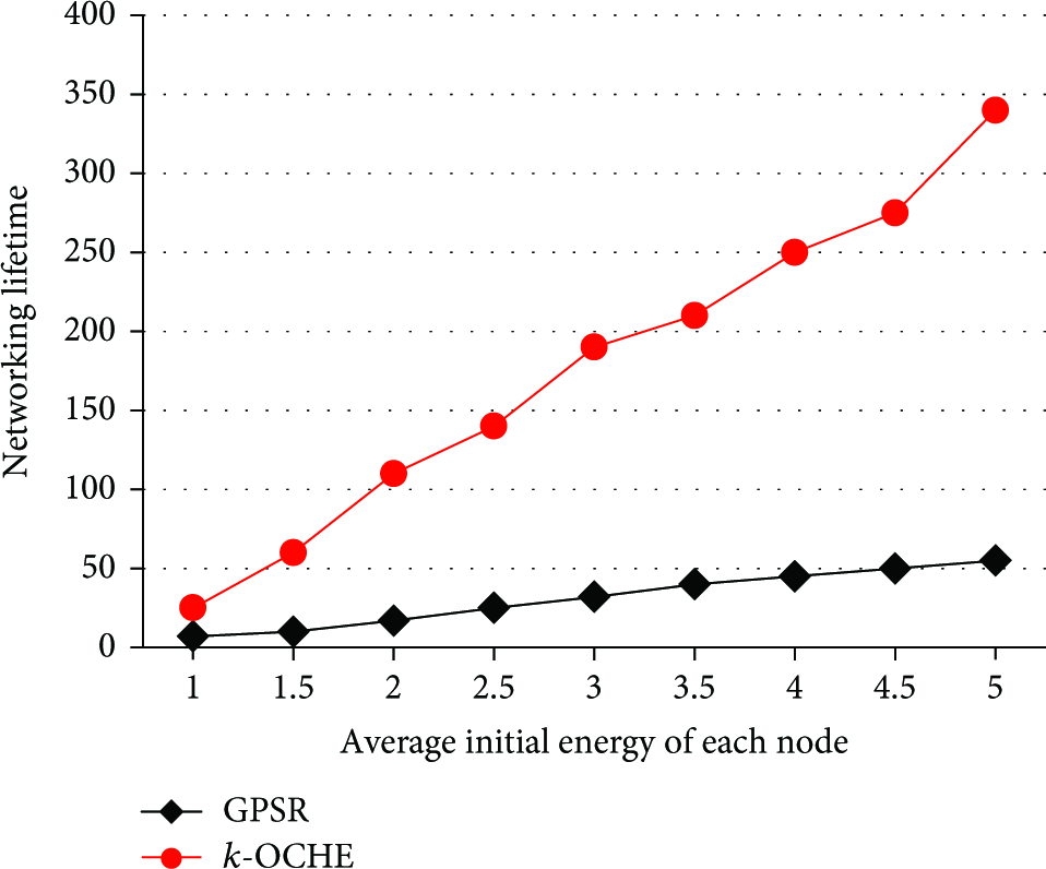
Comparison of network lifetime by using traditional GPSR and k-OCHE-based GPSR.

6.4. Recovery Time

Figure 8 shows the impact of the network size (node density) on the time to repair from an individual node failure for GPSR and k-OCHE, respectively. The x-axis is the network size and the y-axis is the value of recovery time. It is obvious that the recovery time of k-OCHE is much more better than that of GPSR, especially at high values of network size. For low values of network size, that is network size <30, k-OCHE will consume a little bit more recovery time due to the maintenance of clusters. For high values of network size, the recovery time of GPSR increases with network size linearly, while the recovery time of k-OCHE increases very slowly.

Figure 8

Comparison of routing recovery time by using traditional GPSR and k-OCHE-based GPSR.

Figure 9

Demonstration of k-OCHE for different number of nodes n when $k = 3$ .

7. Conclusion

In this paper, we propose a k-connected overlapping clustering approach with energy availability for routing and topology information maintenance in WSNs. We compare k-OCHE with the classical GPSR, and simulation results show that k-OCHE balances the load to extend the lifetime of sensor network. What is more, k-OCHE achieves shorter recovery time than GPSR, especially with large network size.

Footnotes

Appendix

We present the pseudo code of k-OCHE and review Connected K-Neighborhood (CKN) algorithm in [27] in this appendix.

Acknowledgment

This work is supported by the Natural Science Foundation of China under Grants no. 61070181, no. 61272524, and no. 61202442.

References

Yick

Mukherjee

Ghosal

Wireless sensor network survey

Computer Networks 52 12 2292 2330

Akkaya

Younis

A survey on routing protocols for wireless sensor networks

Ad Hoc Networks 2005 3 3 325 349

2-s2.0-13944283393

10.1016/j.adhoc.2003.09.010

Johnsort

Routing in ad hoc networks of mobile hosts

Proceedings of the 1st Workshop on Mobile Computing Systems and Applications (WMCSA ′94)

1994

IEEE

158 163

Soro

Heinzelman

W. B.

Prolonging the lifetime of wireless sensor networks via unequal clustering

Proceedings of the 19th IEEE International Parallel and Distributed Processing Symposium (IPDPS ′05)

April 2005

IEEE

2-s2.0-33746310074

10.1109/IPDPS.2005.365

Chang

J. H.

Tassiulas

Maximum lifetime routing in wireless sensor networks

IEEE/ACM Transactions on Networking 2004 12 4 609 619

2-s2.0-4644360171

10.1109/TNET.2004.833122

Perkins

Bhagwat

Highly dynamic destination-sequenced distance-vector routing (dsdv) for mobile computers

ACM SIGCOMM Computer Communication Review 1994 24 4 234 244

Karp

Kung

H. T.

GPSR: Greedy Perimeter Stateless Routing for wireless networks

Proceedings of the 6th Annual International Conference on Mobile Computing and Networking (MOBICOM ′00)

August 2000

ACM

243 254

2-s2.0-0034547115

Shu

Zhang

Yang

L. T.

Wang

Hauswirth

Xiong

TPGF: geographic routing in wireless multimedia sensor networks

Telecommunication Systems 2010 44 1-2 79 95

2-s2.0-77951880273

10.1007/s11235-009-9227-0

Rodoplu

Meng

T. H.

Minimum energy mobile wireless networks

IEEE Journal on Selected Areas in Communications 1999 17 8 1333 1344

2-s2.0-0032667848

10.1109/49.779917

10.

Heidemann

Estrin

Geography-informed energy conservation for ad hoc routing

Proceedings of the 7th Annual International Conference on Mobile Computing and Networking

July 2001

ACM

70 84

2-s2.0-0034772133

11.

Govindan

Estrin

Geographical and energy aware routing: a recursive data dissemination protocol for wireless sensor networks

2001

Citeseer

12.

Abbasi

A. A.

Younis

A survey on clustering algorithms for wireless sensor networks

Computer Communications 2007 30 14-15 2826 2841

2-s2.0-34548850872

10.1016/j.comcom.2007.05.024

13.

Baker

D. J.

Ephremides

The architectural organization of a mobile radio network via a distributed algorithm

IEEE Transactions on Communications 1981 29 11 1694 1701

2-s2.0-0019633305

14.

Heinzelman

W. R.

Chandrakasan

Balakrishnan

Energy-efficient communication protocol for wireless microsensor networks

Proceedings of the 33rd Annual Hawaii International Conference on System Siences (HICSS ′00)

January 2000

IEEE

2-s2.0-0033877788

15.

Basagni

Distributed clustering for ad hoc networks

Proceedings of the 4th International Symposium on Parallel Architectures, Algorithms, and Networks (I-SPAN ’99)

1999

IEEE

310 315

16.

Manjeshwar

Agrawal

Teen: a routing protocol for enhanced efficiency in wireless sensor networks

Proceedings of the 1st International Workshop on Parallel and Distributed Computing Issues in Wireless Networks and Mobile Computing

2001

17.

Basagni

Distributed and mobility-adaptive clustering for multimedia support in multi-hop wireless networks

Proceedings of the IEEE VTS 50th Vehicular Technology Conference (VTC ′99)

September 1999

IEEE

889 893

2-s2.0-79952179081

10.1109/VETECF.1999.798457

18.

Manjeshwar

Agrawal

Apteen: a hybrid protocol for efficient routing and comprehensive information retrieval in wireless sensor networks

Proceedings of the 16th International Parallel and Distributed Processing Symposium

2002

19.

Younis

Youssef

Arisha

Energy-aware routing in cluster-based sensor networks

Proceedings of the 10th IEEE International Symposium on Modeling, Analysis and Simulation of Computer and Telecommunications Systems (MASCOTS ′02)

2002

IEEE

129 136

20.

Youssef

Younis

Overlapping multihop clustering for wireless sensor networks

IEEE Transactions on Parallel and Distributed Systems 2009 20 12 1844 1856

2-s2.0-74449091634

10.1109/TPDS.2009.32

21.

Lindsey

Raghavendra

Pegasis: power-efficient gathering in sensor information systems

Proceedings of the IEEE Aerospace Conference

2002

IEEE

3 1125

22.

Lindsey

Raghavendra

Sivalingam

K. M.

Data gathering algorithms in sensor networks using energy metrics

IEEE Transactions on Parallel and Distributed Systems 2002 13 9 924 935

2-s2.0-0036766616

10.1109/TPDS.2002.1036066

23.

Youssef

Younis

Arisha

A constrained shortest-path energy-aware routing algorithm for wireless sensor networks

Proceedings of the Wireless Communications and Networking Conference (WCNC ′02)

2002

IEEE

794 799

24.

Subramanian

Katz

An architecture for building selfconfigurable systems

Proceedings of the 1st Annual Workshop on Mobile and Ad Hoc Networking and Computing (MobiHOC ′00)

2000

IEEE

63 73

25.

Kuhn

Wattenhofer

Zhang

Zollinger

Geometric ad-hoc routing: of theory and practice

Proceedings of the 22nd Annual ACM Symposium on Principles of Distributed Computing (PODC ′03)

July 2003

ACM

63 72

2-s2.0-1142305204

26.

Leong

Mitra

Liskov

Path vector face routing: geographic routing with local face information

Proceedings of the 13th IEEE International Conference on Network Protocols (ICNP ′05)

November 2005

IEEE

147 158

2-s2.0-33750949029

10.1109/ICNP.2005.32

27.

Nath

Gibbons

P. B.

Communicating via fireflies: geographic routing on duty-cycled sensors

Proceedings of the 6th International Symposium on Information Processing in Sensor Networks (IPSN ′07)

April 2007

440 449

2-s2.0-35348830482

10.1145/1236360.1236416

28.

Heinzelman

Application-specific protocol architectures for wireless networks [Ph.D. dissertation] 2000

Massachusetts Institute of Technology

29.

Shu

Zhang

Chen

Wang

Hauswirth

Nettopo: beyond simulator and visualizer for wireless sensor networks

Proceedings of the 2nd International Conference on Future Generation Communication and Networking (FGCN ’08)

2008

IEEE

17 20

30.

Chen

Zhao

On the lifetime of wireless sensor networks

IEEE Communications Letters 2005 9 11 976 978

An Overlapping Clustering Approach for Routing in Wireless Sensor Networks

Abstract

1. Introduction

2. Related Work

2.1. Routing Protocols

2.2. Cluster-Based Approach for Routing

3. Assumptions and Notations

3.1. Network Model

3.2. Sleeping Scheduling Model

3.3. Energy Consumption Model

3.4. Notations

4. The k-OCHE Algorithm

4.1. The Proposed Algorithm

Algorithm 1: The k-OCHE algorithm.

Algorithm 2: Connected K neighborhood (CKN).

4.2. Cluster Head Selection Procedure

4.3. Cluster Generation

4.4. An Illustrative Example

5. Routing Algorithm

5.1. Interior Cluster Routing

5.2. Exterior Cluster Routing Construction

5.3. Routing Maintenance

6. Performance Evaluation

6.1. Experiment Setup

6.2. Energy Consumption

6.3. Network Lifetime

6.4. Recovery Time

7. Conclusion

Footnotes

Appendix

Acknowledgment

References