Sage Journals: Discover world-class research

Abstract

In HDLC serial communication protocol, CRC calculation can first process the most or least significant bit of data. Nowadays most CRC calculation is based on the most significant bit (MSB) first processing. An algorithm of the least significant bit (LSB) first processing parallel CRC is proposed in this paper. Based on the general expression of the least significant bit first processing serial CRC, using state equation method of linear system, we derive a recursive formula by the mathematical deduction. The recursive formula is applicable to any number of bits processed in parallel and any series of generator polynomial. According to the formula, we present the parallel circuit of CRC calculation and implement it with VHDL on FPGA. The results verify the accuracy and effectiveness of this method.

1. Introduction

Cyclic redundancy checksum (CRC) is the core computation step of HDLC protocol [1]. CRC is widely used in high-speed data communications systems, such as Asynchronous Transport Modes (ATM), Ethernet wired networks (ieee802.3), WiFi (ieee802.11), and WiMAX (ieee802.16). Now the data processing capacity is growing, which has reached Gb/s. The traditional easy hardware solution for CRC calculation is the Linear Feedback Shift Register (LFSR), which processes bits serially. Although LFSR can work on high frequency, it is relatively slow to calculate CRC. With the development of modern communications, the high rate of data transmission requires speeding up CRC calculation, the speed of this serial implementation is absolutely inadequate in high-speed data communications. In these cases, a parallel computation of the CRC is used widely [2 –10].

CRC calculation can be divided into most or least significant bit first processing. Nowadays most CRC calculation is based on the most significant bit (MSB) first processing [4]. This paper presents the algorithm and implementation of least significant bit first processing parallel CRC. The traditional serial implementation for CRC calculation is the Linear Feedback Shift Register (LFSR); we first analyze the principle of LFSR in this paper. Then, based on the requirement of least significant bit first processing and the incomplete relative theory, we deduce the formula of least significant bit first processing parallel CRC and implement it with FPGA which is widely applicable [11 –14].

2. The Algorithm of Least Significant Bit First Processing Parallel CRC

2.1. The Algorithm of Serial CRC

In typical serial CRC algorithm [1, 10], the computing processes are assuming that the input information is calculated from the MSB. However, in practical application, input data CRC operation may be processed from the lowest bit first. When the least significant bit of the data flow is processed firstly, the corresponding generator polynomial is necessary to reverse order. For example, the antisequence CCITT-16 standard polynomial expressed in binary is 0'8408. Because the structure of serial CRC is only relevant to the generator polynomial and the order of the data processing, in order to get more generic hardware architecture, assuming least bit processing first, the generator polynomial g(x) = x^{m – 1}*g_{m – 1} + x^{m – 2}*g_{m – 2} + … + x*g₁ + g₀, which used the reverse order, the input sequence m(x) = x^{k – 1}*b_{k – 1} + x^{k – 2}*b_{k – 2} + … + x*b₁ + b₀. You can get universal serial hardware structure as shown in Figure 1.

Figure 1:

Universal serial processing hardware architecture of LSB first CRC.

2.2. The Algorithms of Parallel CRC

It is not easy to summarize LSB first with the simple mathematical calculation, but it is an idea to describe in the classic serial feedback shift register implementation (the state diagram shown in Figure 1). The assumptions of generator polynomial and input sequence are the same as above. [x_{m – 1} … x₁x₀] denote the current computing state of CRC, and [x_{m – 1}′ … x₁′x₀′] represent the next calculation state of CRC. [g_{m – 1} … g₁g₀] is polynomial coefficients from high to low. m indicate LSB first input data.

The universal serial hardware architecture described in Figure 1 can be seen as discrete linear time-invariant systems, which is a method of parallel computing. The equation of state can be described as follows:

\begin{matrix} X (i + 1) = F \cdot X (i) + G \cdot U (i), \\ Y (i) = H \cdot X (i) + J \cdot U (i) . \end{matrix}

(1)

In (1), X(i) is the current state of the system, that is, the current CRC operation result. X(i + 1) is the next state of the system, and U represent the system's input, that is, the LSB first processing serial input data. Y is the output of the system, which is the result of CRC operation. As first process LSB, we can see from Figure 1 that the first feedback data is the least significant bit which is calculated firstly. According to the state transition relation as shown in Figure 1, in (1) the state equation as follows:

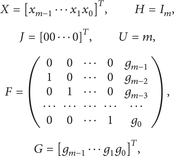
\begin{matrix} X = {[x_{m - 1} \dots x_{1} x_{0}]}^{T}, H = I_{m}, \\ J = {[00 \dots 0]}^{T}, U = m, \\ F = (\begin{pmatrix} 0 & 0 & \dots & 0 & g_{m - 1} \\ 1 & 0 & \dots & 0 & g_{m - 2} \\ 0 & 1 & \dots & 0 & g_{m - 3} \\ \dots & \dots & \dots & \dots & \dots \\ 0 & 0 & \dots & 1 & g_{0} \end{pmatrix}), \\ G = {[g_{m - 1} \dots g_{1} g_{0}]}^{T}, \end{matrix}

(2)

I_m is the identity matrix. Use induction and recursive algorithm to solve this state equation. The operations can be described as follows:

\begin{matrix} X (1) = F \cdot X (0) + G \cdot m (0) = F \cdot (X (0) + {[00 \dots m (0)]}^{T}), X (2) = F \cdot X (1) + G \cdot m (1) \\ = F^{2} \cdot (X (0) + {[00 \dots m (0)]}^{T}) + G \cdot m (1) \\ = F^{2} \cdot (X (0) + {[00 \dots m (1) m (0)]}^{T}); \\ ⋮ \\ X (w) = F^{w} \cdot (X (0) + {[0 \dots 0 ∣ m (w - 1) \dots m (1) m (0)]}^{T}) \\ (when w \leq m) . \end{matrix}

(3)

In (3), ${[0 \dots 0 ∣ \dots]}^{T}$ means to fill zeros before ∣, to make the matrix dimension be m. Equation (3), set matrixM to represent ${[0 \dots 0 ∣ m (w - 1) \dots m (1) m (0)]}^{T}$ ; that is

M = {[0 \dots 0 ∣ m (w - 1) \dots m (1) m (0)]}^{T} .

(4)

We can get the solution of state equation (1) as

X (w) = F^{w} \cdot (X (0) + M); (when w \leq m) .

(5)

w is the width of parallel processing data, m is the degree of the generator polynomial. Through this recursive formula, the CRC can be achieved by one time parallel data processing when w ≤ m. In order to obtain parallel processing of continuous operation CRC recurrence relations, assumptions w = m, because the process of conducting CRC calculation, all calculations are based on modulo 2 arithmetic. The modulo 2 addition is equal to XOR which symbol is ⊕. In Matrix multiplication processing, there are both AND gates to achieve the modulo 2 multiplication and XOR gates to achieve modulo 2 sum, and ⊗ is used to descript this process. Thus, (5) can be expressed as recurrence relations as follows:

\begin{matrix} X^{'} = F^{w} \otimes (X \oplus M), \\ M = {[m (m - 1) \dots m (0)]}^{T}, {[m (2 m - 1) \dots m (m)]}^{T} \dots \\ w = m . \end{matrix}

(6)

According to (6), we derive the recursive formula of parallel CRC when w = m. This is just a special case, for the more general case w < m, just need a little change in the recurrence relations according to (5), that is

\begin{matrix} X^{'} = F^{w} \otimes (X \oplus M); \\ M = {[0 \dots 0 ∣ m (w - 1) \dots m (0)]}^{T}, {[0 \dots 0 ∣ m (2 w - 1) \dots m (w)]}^{T} \dots \\ w < m . \end{matrix}

(7)

According to (6) and (7), we can get the recursive formula of LSB first processing parallel CRC when w ≤ m.

In the above derivation process, the parallel CRC calculation condition for the establishment of recurrence relations is the width of the data w not greater than the degree of generator polynomial m. But that does not mean that the width of the parallel processing of data not greater than degree of generator polynomial. When the width of parallel processing data is greater than the degree of generating polynomial, the data can be divided into several sections so that the width of each section is no greater than the degree of generating polynomial, in resulting CRC computing recurrence relations when w > m. For example, when w = 2m, according to (5), we can derive one time parallel data processing of CRC:

\begin{matrix} X (m) = F^{m} \cdot (X (0) + M {[(m - 1) \dots 0]}^{T}), \\ X (w) = F^{m} \cdot (X (m) + M {[(w - 1) \dots m]}^{T}) \\ = F^{2 m} \cdot (X (0) + M {[(m - 1) \dots 0]}^{T}) \\ + F^{m} \cdot (M {[(w - 1) \dots m]}^{T}) . \end{matrix}

(8)

Using gate function to represent Mode 2 operation, according to (8) and induction method, we can derive recursive formula of parallel CRC when w = 2m:

\begin{matrix} X^{'} = (F^{2 m} \otimes (X \oplus M {[(m - 1) \dots 0]}^{T})) \\ \otimes (F^{m} \otimes (M {[(w - 1) \dots m]}^{T})), \\ M = {[m (w - 1) \dots m (0)]}^{T}, {[m (2 w - 1) \dots m (w)]}^{T} \dots, \\ w = 2 m . \end{matrix}

(9)

And then extend formula to the general situation, let us suppose w = lm + n; 1 ≤ l; 0 ≤ n ≤ m – 1; according to (5), one time parallel process for the CRC operation is as follows:

\begin{matrix} X (w) = (F^{l m + n} \cdot X) + (F^{l m + n} \cdot M {[(m - 1) \dots 0]}^{T}) + \dots \\ + (F^{m + n} \cdot M {[(l m - 1) \dots (l - 1) m]}^{T}) \\ + (F^{n} \cdot M {[0 \dots 0 ∣ (w - 1) \dots l m]}^{T}), \\ M = {[m (w - 1) \dots m (0)]}^{T}, {[m (2 w - 1) \dots m (w)]}^{T} \dots, \\ w = l m + n . \end{matrix}

(10)

According to (10) and induction operations, and use gate function to represent Mode 2 operation in (10), the recursive formula of parallel CRC can be described as follows:

\begin{matrix} X^{'} = (F^{l m + n} \otimes X) \oplus (F^{l m + n} \otimes M {[(m - 1) \dots 0]}^{T}) \\ \oplus \dots \oplus (F^{m + n} \otimes M {[(l m - 1) \dots (l - 1) m]}^{T}) \\ \oplus (F^{n} \otimes M {[0 \dots 0 ∣ (w - 1) \dots l m]}^{T}), \\ M = {[m (w - 1) \dots m (0)]}^{T}, {[m (2 w - 1) \dots m (w)]}^{T} \dots, \\ w = l m + n . \end{matrix}

(11)

From (11), we can get the recursive formula of LSB first processing parallel CRC when w > m, which can be implemented in hardware. In summary, the recursive formula is applicable to any number w of bits processed in parallel and any degree m of the generator polynomial. We can achieve the hardware architecture according to the recurrence relations of (7) and (11).

3. Hardware Architecture of the Parallel CRC Algorithms

Here given the special examples of w ≤ m and w > m, to illuminate hardware implementation structure of LSB first processing parallel CRC.

3.1. w ≤ m Example

Assume generator polynomial use that the reverse order form of CCITT-16 polynomial standard g(x) = x¹⁶ + x¹² + x⁵ + 1, expressed as a binary sequence 0'8408. The width of parallel processing data w = 16, that is w = m. The initial value of the CRC registers 0xffff; that is $X (0) = {[11 \dots 1]}^{T}$ then F in the recurrence relations is

F = [\begin{bmatrix} 0000000000000001 \\ 1000000000000000 \\ 0100000000000000 \\ 0010000000000000 \\ 0001000000000000 \\ 0000100000000001 \\ 0000010000000000 \\ 0000001000000000 \\ 0000000100000000 \\ 0000000010000000 \\ 0000000001000000 \\ 0000000000100000 \\ 0000000000010001 \\ 0000000000001000 \\ 0000000000000100 \\ 0000000000000010 \end{bmatrix}] .

(12)

According to (6), the recurrence relation of parallel computing CRC becomes

\begin{matrix} X^{'} = F^{16} \otimes (X \oplus M), \\ M = {[m (15) \dots m (0)]}^{T}, {[m (31) \dots m (16)]}^{T} \dots, \\ w = m = 16 . \end{matrix}

(13)

The result of F¹⁶ is

F^{16} = [\begin{bmatrix} 1000100010011000 \\ 0100010001001100 \\ 0010001000100110 \\ 0001000100010011 \\ 0000100010001001 \\ 1000110011011100 \\ 0100011001101110 \\ 0010001100110111 \\ 0001000110011011 \\ 0000100011001101 \\ 0000010001100110 \\ 0000001000110011 \\ 1000100110000001 \\ 0100010011000000 \\ 0010001001100000 \\ 0001000100110000 \end{bmatrix}] .

(14)

According to the recurrence relation of (13), we obtain the hardware structure shown in Figure 2.

Figure 2:

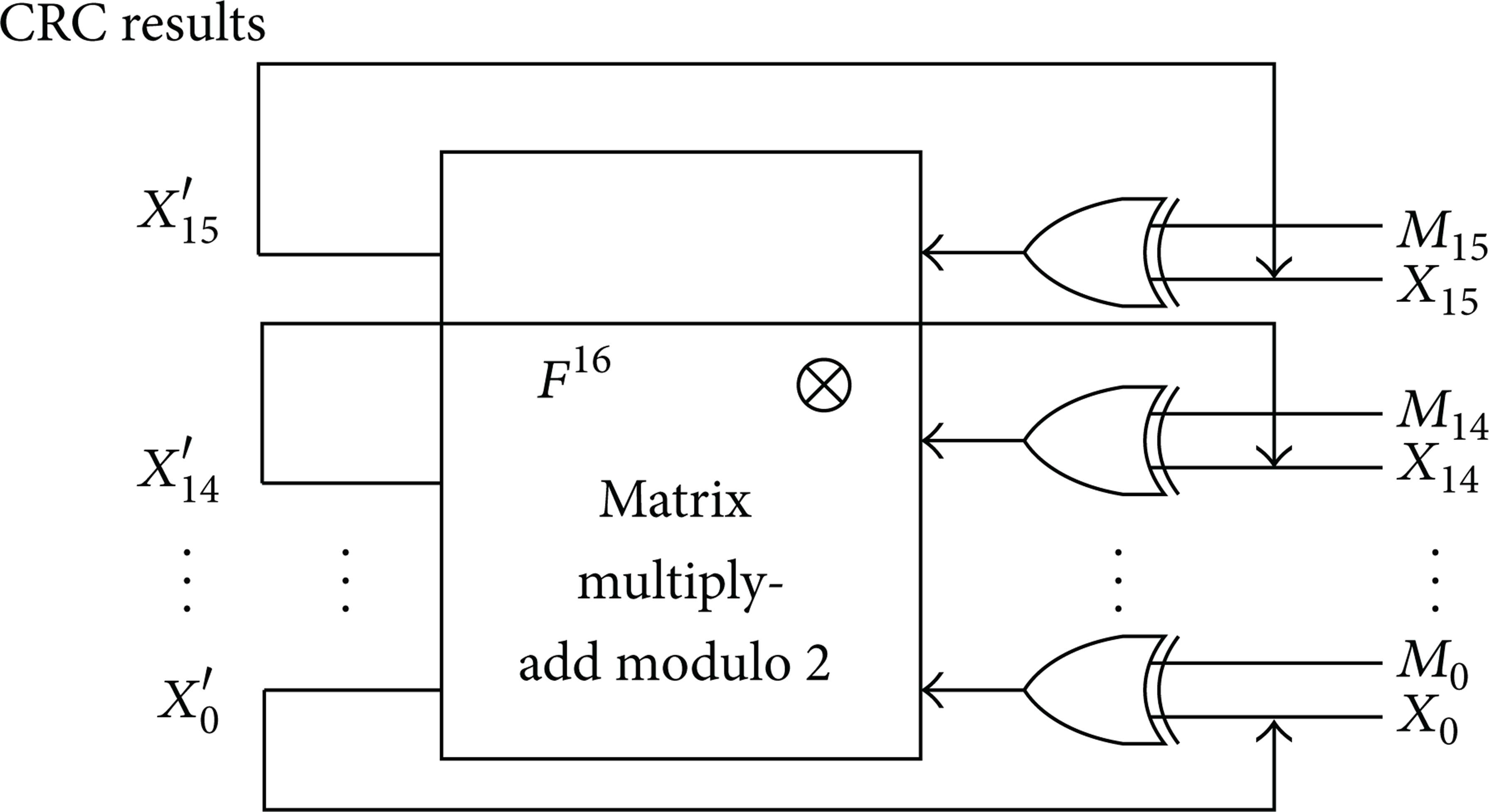
w = m = 16 hardware implementation structure of the parallel CRC.

3.2. w > m Example

Still using the assumptions above, generator polynomial uses the reverse order form of CCITT-16 polynomial standard g(x) = x¹⁶ + x¹² + x⁵ + 1, expressed as a binary sequence 0'8408. The initial value of the CRC registers 0xffff; that is $X (0) = {[11 \dots 1]}^{T}$ . However, the width of parallel processing data isw = 32; that is w = 2m. The following are the principles derivation and implementation of parallel CRC for a special case when the width of parallel processing data w is greater than the degree of generator polynomial.

According to (9), when w = 2m = 32, the recurrence relations of parallel CRC become

\begin{matrix} X^{'} = (F^{32} \otimes (X \oplus M {[15 \dots 0]}^{T})) \oplus (F^{16} \otimes (M {[31 \dots 16]}^{T})), \\ M = {[m (31) \dots m (0)]}^{T}, {[m (63) \dots m (32)]}^{T} \dots, \\ w = 2 m = 32 . \end{matrix}

(15)

Because of the same generating polynomial, matrices F and F¹⁶ are the same as above, but matrix F³² needs to be calculated.

F^{32} = [\begin{bmatrix} 0001101000111000 \\ 0000110100011100 \\ 0000011010001110 \\ 0000001101000111 \\ 1000000110100011 \\ 1101101011101001 \\ 0110110101110100 \\ 0011011010111010 \\ 1001101101011101 \\ 1100110110101110 \\ 1110011011010111 \\ 0111001101101011 \\ 1010001110001101 \\ 1101000111000110 \\ 0110100011100011 \\ 0011010001110001 \end{bmatrix}] .

(16)

From (15), we can obtain the recursive formula of parallel CRC when w = 2m = 32, and the hardware structure is shown in Figure 3.

Figure 3:

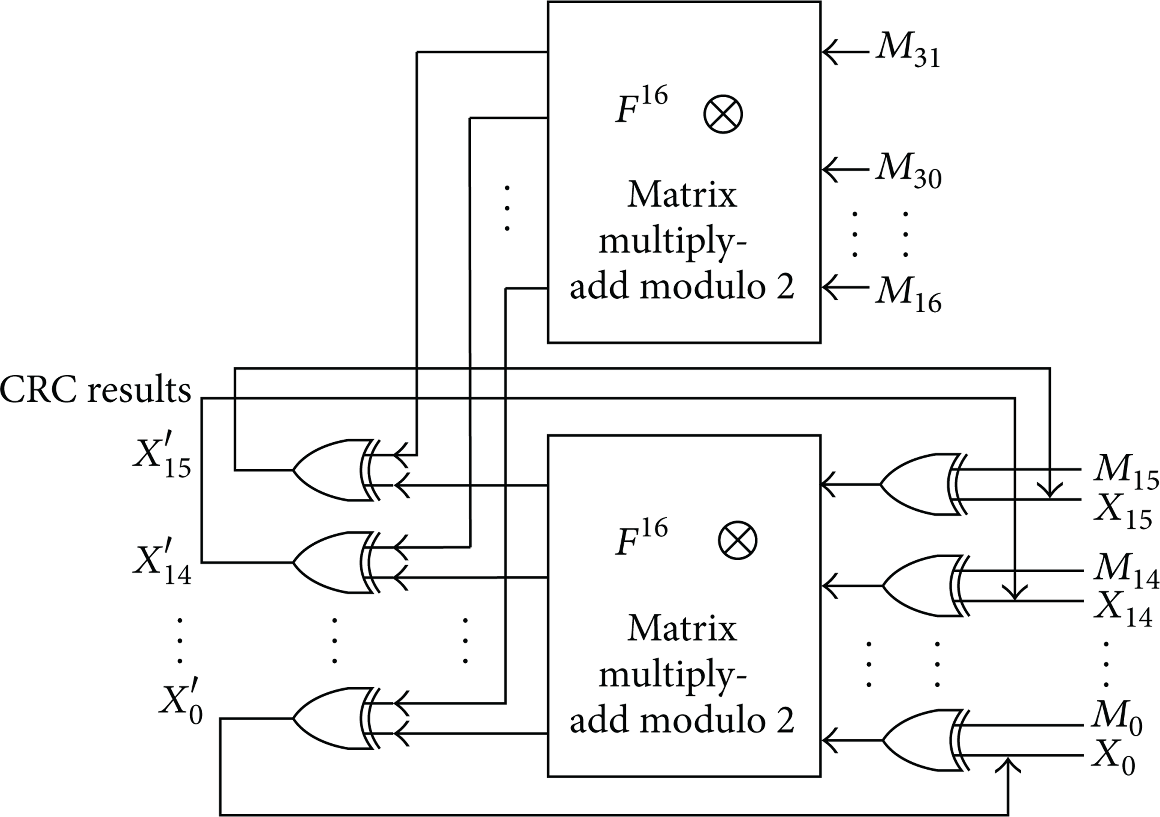
w = 2m = 32 Hardware implementation structure of the parallel CRC.

4. Implementation Results

According to (13) and (15) and the design shown in Figures 2 and 3, implement both w ≤ m and w > m instance, respectively, using the Xilinx V4 series FPGA. Compare experimental results with the literature [4] proposed method and the results are shown in Table 1.

Table 1:

Parallel CRC FPGA resources consumption compare.

	w = m = 16 parallel CRC			w = 2m = 32 parallel CRC
	LUTs	Flip flops	Slices	LUTs	Flip Flops	Slices

This paper LSB first	52	16	18	125	16	59
literature [4] MSB first	78	16	33	140	16	68

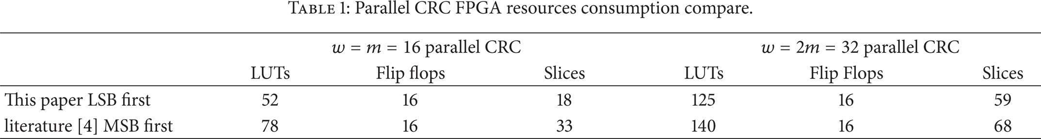
By comparing the data of Table 1 roughly, Table 1 proves that the efficiency of LSB first processing parallel CRC algorithm is more desired. The point of this paper is that the algorithm analyzes both w ≤ m and w > m LSB first processing parallel CRC from the principle.

5. Conclusions

In HDLC serial communication protocol, CRC calculation is the key and usually is implemented by LFSR. With data quantity unceasing increasing and usage of other high-speed communication systems, parallel processing has become as inevitable. In this paper, we firstly analyze the serial implementation of CRC, which uses the serial feedback shift register method. Then, by means of the generic hardware architecture of LSB first processing serial CRC, based on the state equation approach, this paper achieves a LSB first processing parallel CRC algorithm, which is applicable to any number w of bits processed in parallel and any series m of the polynomial generator. Finally, the algorithm is implemented using VHDL programming language on FPGA, which prove its correctness. Comparing FPGA resources consumption with other MSB first processing parallel CRC algorithm proves the effectiveness of the implementation. Error detection performance fully meets actual communication length of 91 Bytes error detection requirements.

References

Peterson

W. W.

and Brown

D. T.

, “Cyclic codes for error detection,” Proceedings of the IRE, vol. 49, no. 1, pp. 228–235, 1961.

Albertengo

and Sisto

, “Parallel CRC generation,” IEEE Micro, vol. 10, no. 5, pp. 63–71, 1990.

Pei

T.-B.

and Zukowski

, “High-speed parallel CRC circuits in VLSI,” IEEE Transactions on Communications, vol. 40, no. 4, pp. 653–657, 1992.

Kennedy

and Arash

R.-M.

, “High-speed parallel crc circuits,” in Proceedings of the 42nd Asilomar Conference on Signals, Systems and Computers (ASILOMAR '08), pp. 1823–1829, October 2008.

Campobello

Patané

, and Russo

, “Parallel CRC realization,” IEEE Transactions on Computers, vol. 52, no. 10, pp. 1312–1319, 2003.

Cheng

and Parhi

K. K.

, “High-speed parallel CRC implementation based on unfolding, pipelining, and retiming,” IEEE Transactions on Circuits and Systems II, vol. 53, no. 10, pp. 1017–1021, 2006.

, and Liu

, “A universal algorithm for parallel CRC computation and its implementation,” Journal of Electronics, vol. 23, no. 4, pp. 528–531, 2006.

Grymel

and Furber

S. B.

, “A novel programmable parallel CRC circuit,” IEEE Transactions on Very Large Scale Integration (VLSI) Systems, vol. 19, no. 10, pp. 1898–1902, 2011.

Sprachmann

, “Automatic generation of parallel CRC circuits,” IEEE Design and Test of Computers, vol. 18, no. 3, pp. 108–114, 2001.

10.

Ramabadran

T. V.

and Gaitonde

S. S.

, “Tutorial on CRC computations,” IEEE Micro, vol. 8, no. 4, pp. 62–75, 1988.

11.

Chen

Zhang

, and Ding

, “Design of dds based on hybird-cordic architecture,” International Journal of Computational Intelligence Systems, vol. 4, no. 3, pp. 306–313, 2011.

12.

Chen

Luo

, and Deng

, “Implementing EW receivers based on large point reconfigured FFT on FPGA platforms,” International Journal of Computational Intelligence Systems, vol. 4, no. 6, pp. 1131–1139, 2011.

13.

Chen

, and Pang

, “Implementation and application of HDLC protocol based on FPGA in radar processing system,” in Proceedings of the International Conference on Electronics, Communications and Control (ICECC '11), pp. 1490–1493, September 2011.

14.

Qiang

and He

, “The design of a large point reconfigured FFT based on FPGA,” in Proceedings of the 2nd International Symposium on Intelligent Information Technology and Security Informatics (IITSI'09), pp. 64–67, January 2009.

A Novel Least Significant Bit First Processing Parallel CRC Circuit

Abstract

1. Introduction

2. The Algorithm of Least Significant Bit First Processing Parallel CRC

2.1. The Algorithm of Serial CRC

2.2. The Algorithms of Parallel CRC

3. Hardware Architecture of the Parallel CRC Algorithms

3.1. w ≤ m Example

3.2. w > m Example

4. Implementation Results

5. Conclusions

References