Sage Journals: Discover world-class research

Abstract

Condition-based monitoring (CBM) has advanced to the stage where industry is now demanding machinery that possesses self-diagnosis ability. This need has spurred the CBM research to be applicable in more expanded areas over the past decades. There are two critical issues in implementing CBM in harsh environments using embedded systems: computational efficiency and adaptability. In this paper, a computationally efficient and adaptive approach including simple principal component analysis (SPCA) for feature dimensionality reduction and K-means clustering for classification is proposed for online embedded machinery diagnosis. Compared with the standard principal component analysis (PCA) and kernel principal component analysis (KPCA), SPCA is adaptive in nature and has lower algorithm complexity when dealing with a large amount of data. The effectiveness of the proposed approach is firstly validated using a standard rolling element bearing test dataset on a personal computer. It is then deployed on an embedded real-time controller and used to monitor a rotating shaft. It was found that the proposed approach scaled well, whereas the standard PCA-based approach broke down when data quantity increased to a certain level. Furthermore, the proposed approach achieved 90% accuracy when diagnosing an induced fault compared to 59% accuracy obtained using the standard PCA-based approach.

1. Introduction

Within the past decades, industrial maintenance has become progressively significant due to the fact that industries are demanding near-zero downtime for operating machines. With the development of sensor and informatics technologies, condition-based maintenance (CBM) approaches have been widely used in various applications [1 –3]. One of the challenges in today's CBM research is that mechanical systems in harsh environments are difficult to be maintained due to their big size, faraway location, and limited accessibility to large-scale computing unit. In addition, some unexpected environmental conditions may accelerate the degradation or failure of mechanical components since their design specifications are based on general environments. These factors will result in a failure to process the collected data efficiently and assess the health status of operating machines adaptively. Specifically, efficiency refers to how to quickly analyze the data with limited computational resources and accurately capture a simple set of features that represents the dynamic characteristics of the operating machine [2]; adaptability means abnormality or faults should be detected in a real-time manner. Thus, an online embedded machinery diagnosis strategy which integrates intelligent feature selection, diagnostic models, and embedded systems needs to be developed to build an on-site knowledge-based platform for machinery fault diagnosis in harsh environments. Although numerous sensor and informatics technologies were applied in fault diagnosis [3 –5], the computational capabilities of embedded systems still cannot meet the requirements when processing a high dimensional dataset. The lack of data computation, transfer speed, and data storage space of equipment in harsh environments can also cause the failure to formulate an optimized online CBM strategy, which has already become a bottleneck problem in many practical situations [6]. Therefore, it is inevitable to find ways to reduce the computational burden of processing high dimensional datasets to realize an optimized online embedded CBM application.

This paper proposes a novel computationally efficient approach which integrates a fast and adaptive feature dimensionality reduction algorithm based on simple principal component analysis (SPCA) and an intelligent K-means clustering algorithm for fault diagnosis. Figure 1 depicts the framework of the proposed approach for online machinery diagnosis. Firstly, raw vibration signals collected from a data acquisition system are analyzed by wavelet analysis, and the energy features are obtained and normalized using z-score method. Secondly, the efficient dimensionality reduction tool, SPCA, is used to simplify the feature space and calculate the principal component vectors. Thirdly, the intelligent K-means clustering algorithm is applied to assess machine performance and diagnose if any faults have happened in a real-time manner [6]. Also, the diagnostic accuracy can be calculated by confusion matrix analysis. The key of this approach is the involvement of computationally efficient algorithms for feature dimensionality reduction and adaptive health assessment, which makes it a suitable approach for online embedded machine diagnosis in harsh environments.

Figure 1:

The framework of the computationally efficient and adaptive approach.

The remainder of this paper is organized as follows. In Section 2, the state-of-art is reviewed for the different dimensional reduction algorithms such as PCA, KPCA, SPCA, and the intelligent K-means clustering algorithm. In Section 3, the mathematical background of PCA, KPCA, and SPCA is introduced with a theoretical analysis of the computational complexity. The potential of SPCA in computational speed and adaptability is discussed. Also, the proposed approach is validated using an offline bearing test dataset. In Section 4, a real online embedded case study is given. The proposed approach is applied to analyze vibration signals that are collected from an imbalanced shaft test rig. The diagnostic results are not only validated, but also benchmarked regarding the calculation speed, as well as the adaptability for the scenario of potentially unknown faults in online embedded CBM applications. Section 5 draws the conclusions.

2. State-of-the-Art

Condition monitoring for a mechanical system usually requires installing some necessary sensors, which result in multiple channels for different signals in the dataset. What's more, even for each channel, applying feature extraction methods in time, frequency, and wavelet domain forms a high dimensional feature matrix, which dramatically increases the data dimension used to describe the condition of the operating machines. This problem will not only create a big burden for all the following data processing, transferring, and storage, but also will hinder the expression for the most useful data information and diagnostic decision making.

Numerous efforts have been targeted on developing dimensionality reduction techniques in the past few decades. Principal component analysis (PCA) is one of the most popular dimension reduction techniques to optimize the features without discarding much original information of the feature space. For instance, Malhi and Gao used PCA to identify the most representative features as inputs to a defect classification application with its ability to discriminate directions with the largest variance in a dataset [7]. Tumer and Huff extracted the principal “modes” of vibrations from the input data for health monitoring of helicopter gearboxes [8]. Khomfoi and Tolbert applied PCA to reduce the number of neurons before neural network classification, and it helped simplify the problem and achieve good results [9]. For studies on fault diagnosis, PCA can be effectively used for feature reduction from the original features [10]. On the other hand, some extensions of PCA were developed for various applications. For example, kernel principal component analysis (KPCA) was proposed to deal with nonlinear problems by characterizing the nonlinearity and nonstationary of industrial systems [11, 12]. Kim et al. applied KPCA to extract facial features and solved face recognition problems [13]. He et al. also established a subspace of feature vectors for gear condition monitoring through KPCA [14]. Researchers have also used KPCA in condition-based monitoring and fault diagnosis applications [15]. Simple principal component analysis (SPCA), invented by Partridge and Calvo [16], was used for dimensionality reduction of two high-dimensional image databases with a fast convergence rate. However, most of the previous studies focused only on the effectiveness of the methods for data dimension reduction in an offline analysis environment. Little attention has been paid to consider if they are still applicable when used in an online embedded CBM application, one of the future mainstreams of CBM research. Even if offline datasets can be used to simulate an online analysis environment for several online CBM methods [6, 17], some problems, such as efficiency and compatibility, can be overlooked very easily without a real online embedded validation.

In this paper, the proposed approach is particularly designed for online embedded machinery CBM applications. The most significant properties of SPCA, computational speed and adaptability, help to improve the data analysis efficiency and adaptively detect abnormality when working with the intelligent K-means clustering algorithm [18] if the machine degradation or fault happens. Further, this study validates the advantages of the approach in an offline fault diagnosis of rolling element bearing and an online embedded imbalanced shaft diagnostic application, respectively.

3. Online Embedded Machinery Diagnosis Approach

3.1. Dimension Reduction

Basically, the methods to calculate the principal components can be divided into two main categories of calculating the eigenvectors. One is based on matrix method, of which a practical technique is applying the singular value decomposition (SVD) technique to calculate principal component vectors. The most commonly used one is the matrix method. For instance, PCA is a technique that can be used to simplify a dataset. More formally it is defined as a linear transformation that chooses a new coordinate system for the dataset such that the greatest variance by any projection of the dataset comes to lay on the first axis, the second greatest variance on the second axis, and so on. Mathematically, PCA converts feature vectors into lower dimensional random variable with independently-distributed components by finding the eigenvalues and eigenvectors of the covariance matrix to represent the statistical significance and directions of principal components, respectively [19]. The detailed steps can be illustrated as follows.

Use x_i to represent the ith sample for the original n-dimensional dataset, i = 1,2, …, m.

Subtract off the mean of each measurement type for the original n-dimensional data matrix X, then the corresponding covariance matrix R = XX^T can be calculated as follows:

R = \sum_{j = 1}^{n} (x_{j} - \overset{—}{x}) {(x_{j} - \overset{—}{x})}^{T} .

(1)

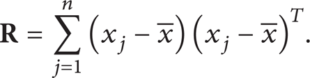
Calculate the eigenvalues λ and eigenvectors ν of R as follows:

λ ν = R ν .

(2)

Sort the eigenvalues and the corresponding eigenvectors, select the first d ≤ n eigenvectors, and generate the new data matrix. Here, d is the number of preferred dimensionality.

Another example of the matrix method to compute eigenvalues and eigenvectors is KPCA, which is an extension of the standard PCA using kernel functions to realize a nonlinear mapping. For KPCA, data in the input space is usually mapped to a higher dimensional feature space where its eigenvectors can be calculated. However, the enhancement for the nonlinear feature of KPCA requires much more computational resources, which may lower the efficiency and make it not suitable for online applications. The algorithm steps of KPCA can be shown as follows.

Use x_i to represent the ith sample for the original n-dimensional dataset, i = 1,2, …, m.

Subtract off the mean of each feature dimension for the original data matrix X.

Project the matrix obtained from step 2 to a higher dimension by using a kernel function and normalize the m-by-m kernel matrix K as follows:

K = k (x_{i}, x_{j}) = Φ (x_{i}) \cdot Φ (x_{j}),

(3)

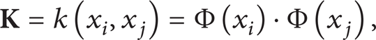
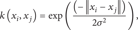
where x_i and x_j are the sample vectors. k is the kernel function. The common kernel functions proposed by Vapnik et al. [20] mainly include polynomial kernel function, radial basis function, and neural network kernel function in (4)–(6), respectively, as follows:

k (x_{i}, x_{j}) = {(x_{i} \cdot x_{j} + 1)}^{d},

(4)

k (x_{i}, x_{j}) = \exp (\frac{(- ∥ x_{i} - x_{j} ∥)}{2 σ^{2}}),

(5)

k (x_{i}, x_{j}) = \tanh ((x_{i} \cdot x_{j}) + b) .

(6)

Calculate the eigenvalues λ and the corresponding eigenvectors ν of the normalized kernel matrix K_n. One has

m λ ν = K_{n} ν .

(7)

Normalize eigenvectors, select the first d ≤ n eigenvectors, and generate the new data matrix.

The second category to determine the principal component vectors is based on the data method. SPCA falls into this category [16]. Compared with the matrix-based methods, the numerical methods can reduce the computational complexity, especially when the dimension of the dataset increases. In SPCA, a data oriented method is adopted to approximate the principal components instead of explicitly calculating the eigenvectors based on the covariance matrix. In addition, SPCA uses a Hebbian-learning-like algorithm to adapt the learning parameters dynamically and quickly find eigenvectors, but avoids the learning parameter tuning problem of the Hebbian learning rule [16]. The procedure of SPCA can be described in Figure 2 and as follows.

Use x_i to represent the ith sample for the original n-dimensional dataset, i = 1,2, …, m.

Subtract off the mean of each measurement type.

Initialize an n-dimensional vector e_k⁰, where k = 1, 2, …, d.

Calculate the kth principal component vector e_k based on the following equations:

y_{i} = \frac{1}{∥ e_{k}^{i - 1} ∥} {(e_{k}^{i - 1})}^{T} x_{i} .

(8)

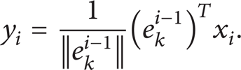
The purpose of (8) is to map the ith sample using the latest kth principal component vector. So y_i is the projection in the direction of kth principal component vector. It can also be viewed as the “similarity” between the ith sample vector and the latest kth principal component vector. One has

ϕ (y_{i}, x_{i}) = y_{i} x_{i} .

(9)

In order to calculate the change of the kth principal component vector, a Hebbian term ϕ(y_i, x_i) is defined in (9). It can be found that the larger y_i is, the more influential the ith sample will be in determining the kth principal component vector. Consider

e_{k}^{i} = \frac{\sum_{i} ϕ (y_{i}, x_{i})}{∥ \sum_{i} ϕ (y_{i}, x_{i}) ∥} .

(10)

Then in (10), the latest kth principal component vector e_kⁱ can be obtained by normalization. The (i + 1) th sample will be used to update the kth principal component vector to e_k^{i + 1}.

Up to this point, the kth principal component vector has been obtained after using all m samples in the kth iteration. In order to find the (k + 1) th principal component vector, the following equation has to be used for all data samples to remove the effect of the kth principal component, so as to avoid being found again:

x_{i}^{'} = x_{i} - (e_{k}^{T} x_{i}) e_{k} .

(11)

Repeat Steps 3–5 untild (d ≤ n) principal component vectors have been obtained. Figure 3 illustrates the graphical steps to find the first principal component vector in SPCA algorithm.

Figure 2:

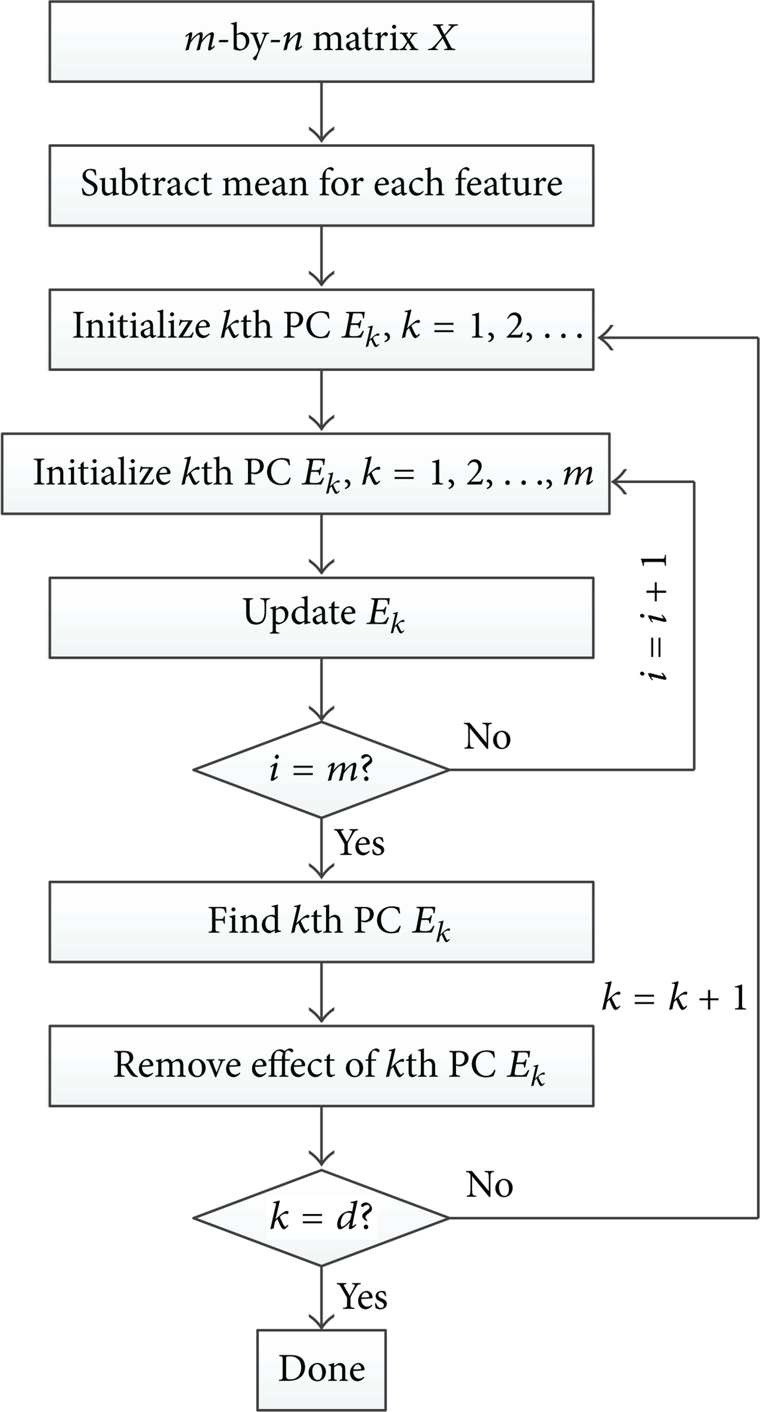
SPCA algorithm procedure.

Figure 3:

SPCA algorithm procedure. (a) Data distribution with an initialized approximate principal component vector; (b) a better approximate principal component vector has been found; and (c) the real first principal component vector of this data distribution is given.

3.2. Dimension Reduction Algorithm Complexity

The computational speed of PCA, SPCA, and KPCA depends on the dimensionality of the feature space. However, it is also affected by different attributes of the input matrix or vectors. For instance, if the objective is to find d (d ≤ n) principal components in an n-dimensional matrix with m samples using PCA, the time complexity for singular value decomposition (SVD) or Householder-QR technique is O(mn² + n³) and for utilizing Hotelling's power method, it is O(mn² + dn²). Additionally, the computation of KPCA realized by calculating eigenvectors involves a time complexity of O(m³) [21], and the time complexity for SPCA is O(dmn) by looking into its computational steps. It can be concluded that the time complexity for PCA increases more dramatically than that of SPCA when the data dimension n gets larger. For KPCA, its calculation speed is slow if the data sample number is large. As a result, implementing PCA or KPCA on large datasets is prohibitively time expensive.

Further, how these variables, that is, target dimensionality, the target number of principal components d, sample number (m), or data matrix dimension (n), influence the time complexity can be studied. PCA, SPCA, and KPCA are applied to a data matrix with randomly generated numbers to study the different computational speeds by changing the row number and the column number from an initial number 100 up to 1000 with an increment of 100 for each step. Figure 4 shows computational speeds for different sizes of the input matrix for PCA, SPCA, and KPCA, respectively.

Figure 4:

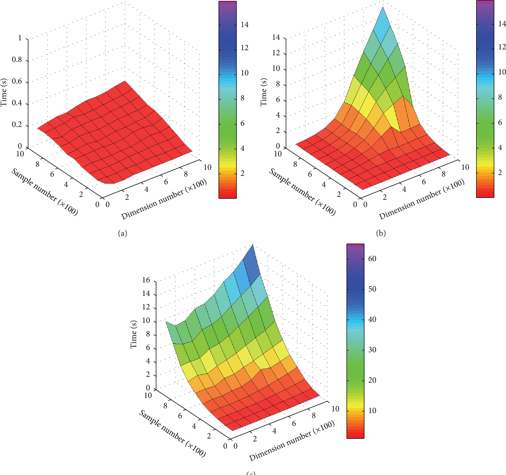
Computational time by: (a) SPCA, (b) PCA, and (c) KPCA.

It can be seen from Figure 4 that the advantage of the computational speed of SPCA gets more apparent when the size of the matrix becomes larger. Its time cost increases much slower than the other two methods do. The computational speed of SPCA is mainly affected by the sample number m, while dimension number n becomes a relatively minor factor, which can be explained by the data-oriented procedure of SPCA. Furthermore, its computational cost is low even when the size of data matrix is very large. Taking the 1000-by-1000 data matrix as an example, the computational time of SPCA is 0.2646 s. It is reduced by 97.8% and 98.4% when compared with PCA (13.110 s) and KPCA (15.957 s), respectively. Similarly, the sample number m is the major factor for KPCA in terms of computational speed. Nonetheless, the computational consumption becomes prohibitively high with the growing sample number m, and it will exceed the consumption of PCA. On the contrary, the computational speed of PCA is determined by the smaller number between row size and column size. For example, if there is an n-dimensional data matrix with m samples (m > n), then n will be the key factor influencing PCA's computational speed. This can be verified by looking into the mathematical steps of PCA, an n-by-n matrix is utilized to calculate the eigenvalues. What's more, the computational time of PCA rises exponentially with the growth of n and will be very slow if n is a large number.

3.3. Online Adaptive Diagnosis Potential of SPCA

For most online monitoring cases, it is desired to find the principal component vectors accurately and quickly with as little computational consumption as possible. However, PCA, as well as KPCA, usually needs all of the data samples to calculate the principal component vectors. Therefore, the computational speed will be very slow when the dataset size is large. This may result in the delay of data processing and significantly weaken the applicability of online analysis.

As previously mentioned, SPCA adopts a data-oriented method to calculate principal component vectors. Thus, it can update the principal component vectors at every iteration, which enables it to utilize the most recent principal component vectors when new data samples come in. This means, it is only necessary to store the latest principal component vectors and discard old data samples instead of saving all data samples to calculate the principal component vectors. As a result, both hardware storage and computational consumption will be saved in embedded systems. Moreover, in some situations where the machine starts to degrade, people may not have the failure data to train the model and use it to detect the degradation or unknown faults quickly, because the principal components vectors are calculated in normal operating conditions. The principal components trained by only normal status data may blur or mislead the clustering results in these cases. To solve it, another way is to train PCA or KPCA frequently to acquire the latest principal component vectors, which is time consuming whenever new data sample comes in and requires a lot of memory to store all the history data. This property of PCA and KPCA will slow down the calculation and may quickly exhaust the computational resources of some embedded systems. Compared with PCA and KPCA, SPCA can always process the new data sample to update the previous-latest principal components. Then, in case new incoming data from some unknown faults is fed into the CBM system, the adaptability of SPCA may help to achieve accurate classification results as well as to identify the new features of the failure status that deviate from the cluster of the normal conditions. It will be shown that this deviation can be viewed as an abnormality or fault indicator by using SPCA instead of PCA and KPCA.

3.4. Offline Approach Validation

Before a real online embedded implementation, the proposed approach is applied in a fault-seeded bearing test. The vibration dataset used in this work is acquired from a standard rolling element bearing test [22] which has been studied by many researchers [6, 23 –25]. The vibration data was acquired by accelerometers at the sampling frequency of 12 KHz. The type of test bearings was the deep groove ball bearing 6205-2RS JEM SKF. During the test, the rotation speed was about 30 Hz (1800 rpm) under different loads (0, 0.75, 1.49 and 2.24 KW).

There are 985 data samples in total from the normal and the fault-seeded bearings. Each data sample has 2048 data points. Among the datasets, there are 276 from the normal conditions, and the rest of 709 samples are of faulty conditions (237 inner race fault samples, 236 outer race fault samples, and 236 ball fault samples). Faults are introduced into either the inner raceways or the outer raceways of the drive-end bearings by the electric discharge machining method. The diameter of the faults is 0.1778 mm with depth of 0.2794 mm.

The second-generation wavelet packet decomposition is used to extract the energy features in the time-frequency domain [6, 26]. Basically, the second generation wavelet transform uses a general construction of the lifting scheme which has three major advantages (1) the fully in-place calculation of wavelet transforms, (2) no requirement for auxiliary memory, and (3) a faster implementation of the wavelet transform [27, 28].

Considering the rotation speed is about 30 Hz and the sampling rate is 12 KHz in this experiment, the decomposition level is chosen to be 7 so that the whole frequency space can be equally divided into 128 intervals. Therefore, the distance between centers of adjacent frequency spans is 46.875 Hz which is close to the normal operating frequency. Thus, the 7-level decomposition of the lifting-based biorthogonal wavelet packet transform is applied to map the raw signals into the wavelet domain, where the packet energy of each decomposition node is calculated and then normalized by the z-score method. Thus, a large matrix of wavelet packet energy for normal condition and three faulty conditions is obtained. The obtained feature space has 128 dimensions.

The datasets are divided into the training sets and the testing sets through a random cross-validation process; 50% of the datasets are used as a training dataset to calculate the principal components. Standard PCA, KPCA, and SPCA are applied to the training dataset, respectively. The result is the product of whole datasets and principal component vectors. For the purpose of visualization, the fault classification results have been plotted (see Figure 5).

Figure 5:

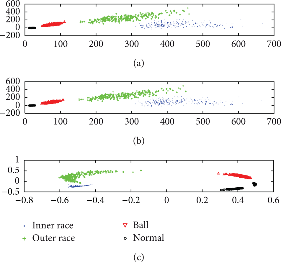
Bearing faults classification. (a) Bearing faults classification using PCA, (b) bearing faults classification using SPCA, and (c) bearing faults classification using KPCA.

It can be seen from Figure 5 that the gaps between each two data clusters are all clear for the applied methods, which indicate that the normal dataset and the three fault datasets can be easily classified. Secondly, the normal datasets scatter much more centralized than the faulty datasets do in the plots of PCA and SPCA, which may reveal an increasing unstableness of the faulty conditions. In addition, as PCA and SPCA share the same objective equations, although with different ways to calculate the principal components, the shapes of the dataset distributions are similar. The distribution shape of the dataset projected by using KPCA is quite different from those done by PCA and SPCA because of its nonlinear property. All the previously mentioned dimension reduction algorithms are effective for the rolling element bearing diagnosis within a 2-dimensional feature space. In other words, 98.44% of redundant data has been eliminated, that is, from 128 dimensions to only 2 dimensions.

3.4.1. Study on Computational Speed for Online Purpose

For a better implementation in online applications, the computational speed of dimension reduction for different data dimensions regarding the scale or size of the input matrix is studied. The feature dimensionality is adjusted by changing the wavelet decomposition level. The results of processing the training dataset are shown in Table 1. To understand how computational time varies intuitively based on the adjustment of wavelet decomposition level, the comparison among the computational time of PCA, SPCA, and KPCA is shown in Figure 6 as follows.

Table 1:

The computational speed of different size of data matrix for 493 feature points.

Wavelet decomposition level	5	6	7	8	9

Feature dimensionality	32	64	128	256	512
SPCA time cost (s)	0.097	0.100	0.104	0.111	0.124
PCA time cost (s)	0.013	0.017	0.041	0.219	1.001
KPCA time cost (s)	0.922	0.946	0.985	1.194	1.422

Figure 6:

The computational time for different wavelet decomposition level (the larger the number wavelet decomposition level is, the higher the dimensionality of the feature space is.)

The observations are:

As wavelet decomposition level changes incrementally, the dimensionality accordingly increases. The sample number remains constant. The increase in computational time of SPCA when dealing with 32-dimensional and 512-dimentional data is 27.83%; For PCA, the increase in the time consumption is 7600%; and for KPCA, it is 54.23%. It can be seen that the increase in time consumption of SPCA is much smaller than that of PCA and KPCA.

Although the computational time for PCA is smaller than that of SPCA when the wavelet decomposition levels are 5, 6, and 7, its speed decreases exponentially with the growing feature dimensionality due to the wavelet decomposition levels increasing to 8 and 9, and quickly goes far beyond the time consumption of SPCA, which corresponds with what has been discussed in Section 3.2.

The computational time of KPCA is usually much more than those of PCA and SPCA, which indicates that KPCA is not quite suitable for an online application that requires a reasonably quick response time to process the data. On the contrary, SPCA can save computational time, especially for large dimensional feature sets, which may entitle SPCA as a sound option of dimension reduction technique to solve the bottleneck problem due to limited computational resources in online applications.

3.4.2. Study on Adaptability for Online Purpose

In many scenarios of real world condition-monitoring applications, the machine runs normally for a long time after it is installed in a manufacturing line. The critical equipment must be regularly maintained to reliably work in its normal status, which means people often lack the data from the faulty status. For this kind of scenario, it is reasonable to assume that the diagnosis algorithms can be trained by only the dataset from the normal status in many cases. Due to the lack of the faulty information, the adaptability is required for the online applications. Therefore, it is necessary to study the adaptability of the algorithms in order to deal with the unknown faults. In this paper, PCA and SPCA are compared by the following procedure.

Step 1. Assume that only the data from the normal status of the machine can be obtained in the initiate operation stage. Thus, the PCA and the SPCA are trained by the dataset of the normal status.

Step 2. Assume that the three seeded fault types (inner race fault, outer race fault, and ball fault) are unknown abnormal statuses, which will occur after the normal status, respectively. Thus, the principal component vectors trained in Step 1 will be applied to the unknown abnormal statuses.

The KPCA is not included in this comparison because of its slow computational response as mentioned in the previous study. The comparison experiment results of the adaptability study are shown in Figures 7, 8, and 9.

Figure 7:

(a) Bearing normal and inner race fault classification using PCA. (b) Bearing normal and inner race fault classification using SPCA.

Figure 8:

(a) Bearing normal and outer race fault classification using PCA. (b) Bearing normal and outer race fault classification using SPCA.

Figure 9:

(a) Bearing normal and ball fault classification using PCA. (b) Bearing normal and ball fault classification using SPCA.

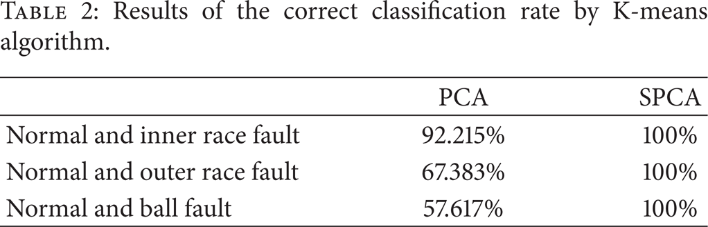
It can be seen from Figures 7, 8, and 9 and Table 2 that when the bearing fault occurs, the normal condition and the faulty condition can hardly be classified by applying PCA, especially for the outer race fault and the ball fault conditions. For the inner race fault, although there are no obvious overlapped clusters, the correct classification rate based on standard PCA is still lower than that based on SPCA. Compared with PCA; the gaps between clusters of feature points from normal and faulty conditions projected by SPCA are much clearer. Therefore, it can be seen that the proposed approach can not only effectively reduce the dimensionality of the feature space, but also adaptively separate the normal condition and the unknown faulty conditions by updating the trained principal component vectors when new data comes in.

Table 2:

Results of the correct classification rate by K-means algorithm.

	PCA	SPCA

Normal and inner race fault	92.215%	100%
Normal and outer race fault	67.383%	100%
Normal and ball fault	57.617%	100%

4. Online Embedded Case Study for Imbalanced Shaft Diagnosis

4.1. Experiment Setup

In this case study, a test rig consisting of a rotating shaft is used for the purpose of validating the advantages of the proposed approach in online embedded CBM applications (see Figures 10 and 11). This test rig consists of a shaft connected to a three-phase industrial motor, a disk attached in the middle of the shaft, two bearings to hold the shaft on each side, and a controller used to set the rotation speed of the shaft. The imbalanced shaft fault can be induced by putting screws into the disk. An accelerometer is mounted on one side of the bearing houses to collect the vibration data.

Figure 10:

Test rig for shaft vibration data acquisition.

Figure 11:

The schematic description of the test rig.

The condition monitoring algorithms are deployed on an embedded system, which consists of an NI cRIO-9004 real-time controller of 64 MB DRAM, 512 MB compact flash, and an NI cRIO-9104 reconfigurable chassis with an NI 9234 IEPE vibration signal collection module. The algorithms are compiled to an FPGA executable LabVIEW program to analyze the data acquired by the NI 9234 module and the accelerometer. The data sampling rate is set at 5120 Hz, and the rotation speed of the shaft is set at 20 Hz (1200 rpm). The embedded system is connected to a computer for displaying the results of real-time monitoring after data processing is finished.

4.2. Study on Online Embedded Computational Speed

The data processing procedure is the same as the procedure described in the previous case study. The computational speed values of PCA and SPCA are compared by analyzing the matrix of the features of the wavelet packet coefficient energies. Different wavelet packet decomposition levels are tried from 5 to 10. The experiment is implemented on 500 feature points. There are 2048 vibration data samples processed for each feature point. The results are shown in Table 3.

Table 3:

Computational speed of different feature dimensionality in the embedded system.

Wavelet decomposition level	5	6	7	8	9	10

Feature dimensionality	32	64	128	256	512	1024
SPCA time cost (s)	0.162	0.275	0.477	0.913	1.767	3.636
PCA time cost (s)	0.376	1.249	5.640	32.787	N/A	N/A

With the increase of wavelet decomposition level, it can be seen that SPCA deployed on the embedded system is still able to reduce the feature dimensionality with limited computational resources when data dimensionality gets higher. Nevertheless, the computational time for PCA goes up exponentially again with increasing dimensionality of the feature vectors when the wavelet packet decomposition level changes from 5 to 8. Out-of-memory errors occur on the embedded system when the wavelet decomposition level further increases to 9 and 10, which makes the results not available (N/A). Further, if Table 3 is compared with Table 1, efficiency of SPCA becomes much more outstanding in a real online embedded implementation, while the usage of PCA can result in a long delay or even breakdown which will weaken the significance of online data processing and timely decision making.

4.3. Study on Adaptability for Online Embedded Application

Besides the scenario of limited online computational resources for the embedded system, another online scenario is lacking the faulty information when the diagnosis algorithm is deployed and applied, which means that the adaptability for an unknown faulty status is required. An online analysis scenario is assumed that people are unaware of the coming faults (to be induced) in the beginning when the algorithms are deployed on the embedded system. Thus, the principal component vectors of standard PCA and SPCA are trained by the normal condition and applied to all the new incoming data, including from the normal and the faulty statuses. The detailed procedure is shown as follows.

Collect and process the data from normal shaft, and train the principal component vectors using standard PCA and SPCA.

Induce the imbalanced shaft fault by putting screws into the disk.

Collect and process the data from the faulty shaft, and reduce its dimensionality using the trained principal component vectors.

Visualize the projected feature points of both normal and faulty conditions.

Considering the rotation speed is about 20 Hz and the sampling rate is 5.12 KHz in the experiment, the decomposition level is chosen to be 7 so that the whole frequency space can be equally divided into 128 intervals, of which the distance between centers of adjacent frequency spans is 20 Hz which is the same as the normal operating frequency. The test has been run ten times for the purpose of validation. The screenshots of the visualization step during one of the ten tests are shown in Figures 12 and 13. The separation between the normal cluster and the faulty cluster mapped by SPCA is much clearer than that mapped by standard PCA.

Figure 12:

Online shaft diagnosis using PCA.

Figure 13:

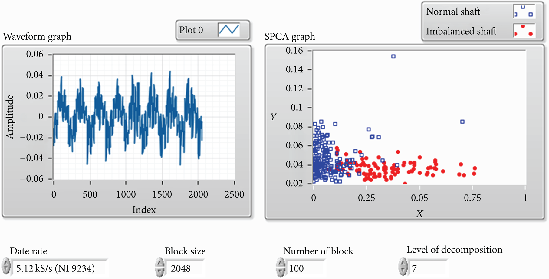
Online shaft diagnosis using SPCA.

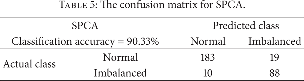
To find out quantitative classification accuracy for each online analysis scenario, K-means clustering algorithm is used to cluster the feature points from normal and imbalanced faulty statuses, and the diagnosis accuracy in one of the tests is shown in confusion matrices in Tables 4 and 5. The average accuracies for all the tests are 89.80% for SPCA and 60.80% for standard PCA, respectively. The reason why SPCA can detect the faulty condition with better accuracy than standard PCA in online analysis scenario is because it can utilize the previous principal component vectors and update them adaptively when new data comes in instead of using all data samples to calculate principal component vectors again. Therefore, the proposed approach could not only save computational resources and data storage space, but also improve the machine fault diagnosis efficiency and accuracy in online embedded CBM applications.

Table 4:

The confusion matrix for PCA.

PCA		Predicted class
Classification accuracy = 59.00%		Normal	Imbalanced

Actual class	Normal	139	61
Actual class	Imbalanced	62	38

Table 5:

The confusion matrix for SPCA.

SPCA		Predicted class
Classification accuracy = 90.33%		Normal	Imbalanced

Actual class	Normal	183	19
Actual class	Imbalanced	10	88

5. Conclusion and Future Work

The paper proposes a computationally efficient and adaptive approach which includes SPCA for feature dimensionality reduction and intelligent K-means clustering for online machine faults diagnosis. The approach is applied to an offline rolling element bearing fault diagnosis test and an online embedded imbalanced shaft fault diagnosis application. While it has been demonstrated that the proposed approach is effective in both applications, it is also validated despite the computational constraints which can be easily neglected in simulated online applications. Results show that the proposed approach runs much faster and is more memory saving for high dimensional datasets and has better adaptability to identify the new unknown abnormal or faulty conditions.

In summary, it can be concluded that the proposed approach is a suitable method for online embedded machinery diagnosis applications in harsh environments. Also, a further study will be conducted on some possible ways to realize machine failure mode identification and remaining useful life prediction in the future.

References

Lee

Djurdjanovic

Qiu

, and Liao

, “Intelligent prognostics tools and e-maintenance,” Computers in Industry, vol. 57, no. 6, pp. 476–489, 2006.

and Tso

S. K.

, “Real-time tool condition monitoring using wavelet transforms and fuzzy techniques,” IEEE Transactions on Systems, Man and Cybernetics C, vol. 30, no. 3, pp. 352–357, 2000.

Jardine

A. K. S.

Lin

, and Banjevic

, “A review on machinery diagnostics and prognostics implementing condition-based maintenance,” Mechanical Systems and Signal Processing, vol. 20, no. 7, pp. 1483–1510, 2006.

Tran

V. T.

and Yang

, “An intelligent condition-based maintenance platform for rotating machinery,” Expert Systems with Applications, vol. 39, no. 3, pp. 2977–2988, 2012.

Tran

V. T.

Thom Pham

Yang

B. S.

, and Tien Nguyen

, “Machine performance degradation assessment and remaining useful life prediction using proportional hazard model and support vector machine,” Mechanical Systems and Signal Processing, vol. 32, pp. 320–330, 2012.

Huang

Liu

Zha

X. F.

, and Li

, “A lean model for performance assessment of machinery using second generation wavelet packet transform and Fisher criterion,” Expert Systems with Applications, vol. 37, no. 5, pp. 3815–3822, 2010.

Malhi

and Gao

R. X.

, “PCA-based feature selection scheme for machine defect classification,” IEEE Transactions on Instrumentation and Measurement, vol. 53, no. 6, pp. 1517–1525, 2004.

Tumer

I. Y.

and Huff

E. M.

, “Analysis of triaxial vibration data for health monitoring of helicopter gearboxes,” Journal of Vibration and Acoustics, Transactions of the ASME, vol. 125, no. 1, pp. 120–128, 2003.

Khomfoi

and Tolbert

L. M.

, “Fault diagnosis and reconfiguration for multilevel inverter drive using AI-based techniques,” IEEE Transactions on Industrial Electronics, vol. 54, no. 6, pp. 2954–2968, 2007.

10.

Zhang

, and Zi

, “Fault diagnosis of rotating machinery based on improved wavelet package transform and SVMs ensemble,” Mechanical Systems and Signal Processing, vol. 21, no 2, pp 688–705, 2007.

11.

Schölkopf

Smola

, and Müller

, “Nonlinear component analysis as a Kernel Eigenvalue problem,” Neural Computation, vol. 10, no. 5, pp. 1299–1319, 1998.

12.

Schölkopf

Mika

Burges

C. J. C.

, “Input space versus feature space in Kernel-based methods,” IEEE Transactions on Neural Networks, vol. 10, no. 5, pp. 1000–1017, 1999.

13.

Kim

K. I.

Jung

, and Kim

H. J.

, “Face recognition using Kernel principal component analysis,” IEEE Signal Processing Letters, vol. 9, no. 2, pp. 40–42, 2002.

14.

Kong

, and Yan

, “Subspace-based gearbox condition monitoring by Kernel principal component analysis,” Mechanical Systems and Signal Processing, vol. 21, no. 4, pp. 1755–1772, 2007.

15.

Sun

Tsung

, and Qu

, “Evolving Kernel principal component analysis for fault diagnosis,” Computers and Industrial Engineering, vol. 53, no. 2, pp. 361–371, 2007.

16.

Partridge

and Calvo

R. A.

, “Fast dimensionality reduction and simple PCA,” Intelligent Data Analysis, vol. 2, no. 1–4, pp. 203–214, 1998.

17.

Wang

, and Lee

, “An online adaptive condition-based maintenance method for mechanical systems,” Mechanical Systems and Signal Processing, vol. 24, no. 8, pp. 2985–2995, 2010.

18.

Lloyd

, “Least squares quantization in PCM,” IEEE Transactions on Information Theory, vol. IT-28, no. 2, pp. 129–137, 1982.

19.

Shlens

, “A tutorial on principal component analysis,” Measurement, vol. 51, no. 10003, p. 52, 2005.

20.

Vapnik

Golowich

S. E.

, and Smola

, “Support vector method for function approximation, regression estimation, and signal processing,” Advances in Neural Information Processing Systems, pp. 281–287, 1997.

21.

Tat-Jun

and Suter

, “Improving the speed of Kernel PCA on large scale datasets,” in Proceedings of the IEEE International Conference on Video and Signal Based Surveillance (AVSS '06), p. 41, November 2006.

22.

Loparo

K. A.

, “Bearing Data Center, Case Western Reserve University, United States,” http://www.eecs.case.edu/laboratory/bearing/, 2011.

23.

Liu

, and Huang

, “Adaptive feature extraction using sparse coding for machinery fault diagnosis,” Mechanical Systems and Signal Processing, vol. 25, no. 2, pp. 558–574, 2011.

24.

Gryllias

K. C.

and Antoniadis

I. A.

, “A Support Vector Machine approach based on physical model training for rolling element bearing fault detection in industrial environments,” Engineering Applications of Artificial Intelligence, vol. 25, no. 2, pp. 326–344, 2012.

25.

Ocak

and Loparo

K. A.

, “Estimation of the running speed and bearing defect frequencies of an induction motor from vibration data,” Mechanical Systems and Signal Processing, vol. 18, no. 3, pp. 515–533, 2004.

26.

Hongkai

Zhengjia

Chendong

, and Peng

, “Gearbox fault diagnosis using adaptive redundant Lifting Scheme,” Mechanical Systems and Signal Processing, vol. 20, no. 8, pp. 1992–2006, 2006.

27.

Sweldens

, “The lifting scheme: a construction of second generation wavelets,” SIAM Journal on Mathematical Analysis, vol. 29, no. 2, pp. 511–546, 1998.

28.

Sweldens

, “Lifting scheme: a new philosophy in biorthogonal wavelet constructions,” in Proceedings of the Wavelet Applications in Signal and Image Processing III. Part1 (of 2), pp. 68–79, San Diego, Calif, USA, July 1995.

A Computationally Efficient and Adaptive Approach for Online Embedded Machinery Diagnosis in Harsh Environments

Abstract

1. Introduction

2. State-of-the-Art

3. Online Embedded Machinery Diagnosis Approach

3.1. Dimension Reduction

3.2. Dimension Reduction Algorithm Complexity

3.3. Online Adaptive Diagnosis Potential of SPCA

3.4. Offline Approach Validation

3.4.1. Study on Computational Speed for Online Purpose

3.4.2. Study on Adaptability for Online Purpose

4. Online Embedded Case Study for Imbalanced Shaft Diagnosis

4.1. Experiment Setup

4.2. Study on Online Embedded Computational Speed

4.3. Study on Adaptability for Online Embedded Application

5. Conclusion and Future Work

References