Uncertainty-Aware Sensor Deployment Strategy in Mixed Wireless Sensor Networks

Abstract

Deployment is a fundamental issue in wireless sensor networks (WSNs), which affects the performance and lifetime of the networks. Usually the sensor locations are precomputed based on “perfect” sensor detection model, whereas sensors may not always provide reliable information, either due to operational tolerance levels or environmental factors. Therefore, it is very important to take into account this uncertainty in the deployment process. In this paper, we address the problem of sensor deployment in a mixed sensor network where the mobile and static nodes work collaboratively to perform deployment optimization task. We consider the Gaussian white noise in the environment and present a centralized algorithm (FABGM for short) which discoveres vacancies by using detection model based on false alarm and moves the mobile nodes according to the method based on bipartite graph matching in this study. In this algorithm, the management node of the WSNs collects the geographical information of all of the static and mobile sensors. Then, the management node executes the algorithm to get the best matches between mobile sensors and coverage holes. Simulation results are presented to demonstrate the effectiveness of the proposed approach.

1. Introduction

Wireless sensor networks have received intensive research interest in recent years due to their potential capability of monitoring real physical environments and collecting data. WSNs have been used in various applications, such as forest monitoring, precision agriculture [1], battlefield surveillance, and target tracking. However, in order to conduct their tasks successfully, it is very important that they be deployed properly.

Sensor deployment is at the initial stages in sensor networks research. It is an important issue which has attracted much attention in recent years [2]. The number and locations of sensors deployed in a Region of Interest (RoI) determine the topology of the network, which will further influence many of its intrinsic properties, such as its coverage, connectivity, cost, and lifetime. Consequently, the performance of a sensor network depends to a large extent on its deployment. A problem which impinges upon the success of any WSNs deployment is the fact that sensory data are marred by the flaw of uncertainty. Indeed, information provided by sensors may not always reliable, either due to environmental factors such as Gaussian white noise or operational tolerance levels. Therefore, it is very important to take into account this uncertainty in the deployment process.

However, WSNs cannot be deployed manually in many working environments, such as remote mountainous regions, battlefields, and regions polluted by poisonous gases. An alternative method is scattering the sensors randomly, but this is affected by many uncontrollable factors, and it is difficult to achieve the desired deployment. In the last decade, researchers have focused on mixed sensor networks, in which the static nodes and mobile nodes work in a collaborative fashion to perform deployment task. Such networks have the advantage of mobility so they can be moved to appropriate positions to enhance the extent of coverage and reduce the number of nodes.

In this work, we explore the problem of uncertainty-aware deployment in mixed wireless sensor networks. The original contributions of this work are the following: first, we introduce a false alarm based detection model; a model considers the existence of Gaussian white noise. Second, using the detection model we compute joint detection probability to discover the coverage vacancies. And then, we present an approach which is based on bipartite graph matching to determine the position of the mobile sensor nodes. Before a mobile node moves to coverage vacancy, it will determine whether there are static nodes within its sensing range. If there are static nodes within its sensing range, it moves to the coverage vacancy. Otherwise, it remains in its current position. Experimental results are given to demonstrate the efficiency of our approach.

The remainder of this paper is organized as follows. Section 2 explains related works. Section 3 gives an overview of the false alarm based detection model, and we detail our deployment algorithm in Section 4. Section 5 presents our experiments. This paper is concluded in Section 6.

2. Related Prior Works

According to the characteristics of the nodes that comprise WSNs, there are three types of such networks, that is, (1) static WSNs, in which all the nodes are static; (2) mobile WSNs, in which all the sensors are mobile; and (3) mixed WSNs, in which some of the nodes are static and some are mobile.

The greatest weakness of a random static WSN is that there must be significant redundancy among the nodes in order to achieve good coverage. And the deployment of a deterministic static WSN is inefficient. In [3], the authors use a sequential deployment of sensors that is, a limited number of sensors; are deployed in each step until the desired probability of detection of a target is achieved. Sensor placement on two- and three-dimensional grids was formulated as a combinatorial optimization problem and solved using integer linear programming [4]. The main drawbacks of these approaches are that the grid coverage approach relies on “perfect” sensor detection; that is, a sensor is expected to yield a binary yes/no detection outcome in every case. The authors in [5] provide a polynomial-time, greedy, iterative algorithm to determine the best placement of one sensor at a time in a grid based scenario, such that each grid is covered with a minimum confidence level. Uncertainty associated with the predetermined sensor locations is considered in [6]. The authors propose two sensor placement algorithms, where the sensor location is modeled as a random variable with a Gaussian probability distribution. In [7, 8], the authors define an evidence-based coverage model and conceive an uncertainty-aware deployment algorithm, which determines the minimum number of sensors and their locations to ensure full area coverage. The evidence-based sensor coverage model is a generalization of the probabilistic model.

In mobile WSNs, a fundamental issue is the coverage problem. Many techniques have been developed to deal with this issue, such as coverage pattern-based movement [9–12], virtual force-based movement [13, 14], and Voronoi-based movement [15]. A distributed energy-efficient deployment algorithm is proposed by Heo and Varshney [9]. The goal is the formation of an energy-efficient node topology for a longer system lifetime. In order to achieve this goal, they employ a synergistic combination of cluster structuring and a peer-to-peer deployment scheme. Moreover, an energy-efficient deployment algorithm based on Voronoi diagrams is also proposed here. The authors in [13] propose a deployment strategy to enhance coverage after an initial random placement of sensors using virtual forces. A cluster head computes the new locations of all the sensors after an initial deployment that would maximize coverage, and then nodes reposition themselves to the designated locations. Wang et al. [15] use Voronoi diagrams to discover the coverage vacancies and design three movement-assisted sensor deployment protocols, including VEC (vector based), VOR (Voronoi based), and minimax. The greatest weakness of a mobile WSN is its price, which is significantly greater than the price of a static WSN, because the price of mobile sensors is much greater than the price of static sensors.

The mixed wireless sensor networks that are composed of a mixture of mobile and static sensors are the tradeoff between cost and coverage. To provide the required high coverage, the mobile sensors have to move from dense areas to sparse areas. In [16], the authors proposed a collaborative coverage enhancing algorithm (coven) which uses a “Voronoi polygon” to determine the placed positions and the number of estimated holes. However, it is not feasible to apply Voronoi diagrams in WSNs due to their excessive complexity. A grid deployment method is proposed in [17], where the map is divided into multiple individual grids, and the weight of each grid is determined by environmental factors such as predeployed nodes, boundaries, and obstacles. The grid with minimum values is the goal of the mobile node. The authors in [18] proposed a novel, centralized algorithm to deploy a mixture of mobile and static sensors to construct sensor networks which used Delaunay triangulation rather than a Voronoi diagram to detect the coverage holes.

To the best of our knowledge, almost all related works assume either a binary or a probabilistic-based coverage model. The binary coverage model is overly simplistic and does not reflect reality, while the probabilistic coverage model is limited and does not allow the easy integration of some related issues, such as sensor reliability. This paper presents a centralized algorithm in which the management node executed the algorithm to discover vacancies by using detection model based on false alarm and then to get the best matches between mobile sensors and coverage holes. The detection model used in our work considers the environment factor and reflects reality well. Simulation results show the effectiveness of our algorithm.

3. Detection Model

3.1. Assumptions

Our algorithm is based on the following assumptions.

• (i)

The location of each sensor node is known, which can be obtained at a low cost from Global Positioning System (GPS) or through location discovery algorithms.

(ii)

It is assumed that all sensor nodes have identical capability for sensing and communication.

(iii)

The mobile nodes have the ability to move and can move to the optimized position accurately.

3.2. Sensor Detection Model

We assume that the WSNs work in an environment with a Gaussian white noise, and each sensor involved in the signal detection transmits a signal with the same energy $e_{\mathrm{tr}}$ . Thus, the signal received at a distance of r meters away will have energy of $e_{\mathrm{tr}}/r^{\gamma }$ . Here, a simple geometric path loss model [19] is assumed, and the path loss is proportional to $\mathrm{1}/r^{\gamma }$ , where γ is the path loss exponent, which is an environment-dependent constant typically between 2 and 4. We assume that the number of sensors which perform signal detection is n. Thus, at sensor i, the observations under the two different hypotheses are given by [20]

$$\begin{array}{cc}& y_i=\{\begin{array}{cc}\frac{\beta }{D_{ti}^{\gamma /\mathrm{2}}}+n_i\hfill & H_{\mathrm{1}},\hspace{0.17em}\hspace{0.17em}i=\mathrm{1,2},\dots ,n,\hfill \\ n_i\hfill & H_{\mathrm{2}},\hspace{0.17em}\hspace{0.17em}i=\mathrm{1,2},\dots ,n,\hfill \end{array}\end{array}$$

(1)

where $H_1$ denotes the target-present hypothesis, and $H_0$ is the null hypothesis; $y_i$ is the received signal; $n_i$ is zero-mean, complex Gaussian noise with variance ${\sigma }^2$ ; β is a scalar defined by $\beta =\sqrt{e_{\mathrm{tr}}/{\mathrm{2}}^{\gamma }}$ ; and $D_{ti}$ denotes the distance between the target $(x_t,y_t)$ and the sensor $(x_i,y_i)$ ; that is,

$$\begin{array}{cc}& D_{ti}=\sqrt{{\left(x_t-x_i\right)}^{\mathrm{2}}+{\left(y_t-y_i\right)}^{\mathrm{2}}}.\end{array}$$

(2)

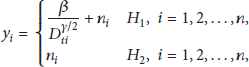
It is noted that under hypothesis $H_{\mathrm{1}}$ , the distance that the active sensing signal traverses is given by $r=\mathrm{2}{D}_{ti}$ . Therefore, for the ith sensor, the likelihood (probability density function) under $H_{\mathrm{1}}$ is given by

$$\begin{array}{cc}& \text{Pr}\left(y_i\mid H_{\mathrm{1}}\right)=\frac{\mathrm{1}}{\sqrt{\mathrm{2}\pi {\sigma }^{\mathrm{2}}}}\exp \left\{-\frac{\mathrm{1}}{\mathrm{2}{\sigma }^{\mathrm{2}}}{\left(y_i-\frac{\beta }{D_{ti}^{\gamma /\mathrm{2}}}\right)}^{\mathrm{2}}\right\},\end{array}$$

(3)

and the likelihood under $H_{\mathrm{0}}$ is

$$\begin{array}{cc}& \text{Pr}\left(y_i\mid H_{\mathrm{0}}\right)=\frac{\mathrm{1}}{\sqrt{\mathrm{2}\pi {\sigma }^{\mathrm{2}}}}\exp \left\{-\frac{y_i^{\mathrm{2}}}{\mathrm{2}{\sigma }^{\mathrm{2}}}\right\}.\end{array}$$

(4)

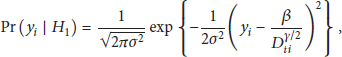
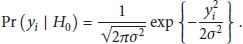
Now, let us focus on the Neyman-Pearson criterion. The Neyman-Pearson criterion maximizes the probability of detection $P_D$ subject to a predetermined bound on the probability of false alarm $P_F$ . In other words, the optimal decision rule ϑ according to the Neyman-Pearson criterion is the solution to the following constrained optimization problem [21]:

$$\begin{array}{cc}& \underset{\vartheta }{\max }\hspace{0.17em}{P}_D\left(\vartheta \right)\mathrm{\hspace{0.17em}\hspace{0.17em}}\text{subject}\mathrm{\hspace{0.17em}\hspace{0.17em}}\text{to}\mathrm{\hspace{0.17em}\hspace{0.17em}}{P}_F\left(\vartheta \right)\le \alpha .\end{array}$$

(5)

The Neyman-Pearson optimum test is a likelihood ratio test [13]. From (3) and (4), the likelihood ratio for sensor i can be written as

$$\begin{array}{l}{L}_i\left(y_i\right)=\frac{P_r\left(y_i\mid H_{\mathrm{1}}\right)}{P_r\left(y_i\mid H_{\mathrm{0}}\right)}\\ \hspace{1em}\hspace{1em}\hspace{0.17em}\hspace{0.17em}=\exp \left\{\frac{\mathrm{1}}{\mathrm{2}{\sigma }^{\mathrm{2}}}\left(\frac{\mathrm{2}\beta y_i}{D_{ti}^{\gamma /\mathrm{2}}}-\frac{{\beta }^{\mathrm{2}}}{D_{ti}^{\gamma }}\right)\right\}.\end{array}$$

(6)

Since the $n_i,i\in [1,n]$ , are assumed to be statistically independent, the joint probability of the observations is simply the product of the individual probability densities. Thus, let us define $y=[y_{\mathrm{1}},\dots ,y_n]$ , for the n sensors, the overall likelihood ratio is

$$\begin{array}{cc}& L\left(y\right)={\displaystyle \prod }_{i=\mathrm{1}}^n{L}_i\left(y_i\right).\end{array}$$

(7)

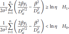
For convenience, we consider the log-likelihood ratio, which is given by

$$\begin{array}{l}\ln \hspace{0.17em}L\left(y\right)={\displaystyle \sum }_{i=\mathrm{1}}^n\ln L_i\left(y_i\right)\\ \hspace{1em}\hspace{1em}\hspace{1em}=\frac{\mathrm{1}}{\mathrm{2}{\sigma }^{\mathrm{2}}}{\displaystyle \sum }_{i=\mathrm{1}}^n\left(\frac{\mathrm{2}\beta y_i}{D_{ti}^{\gamma /\mathrm{2}}}-\frac{{\beta }^{\mathrm{2}}}{D_{ti}^{\gamma }}\right).\end{array}$$

(8)

Therefore, the likelihood ratio test is given by [21]

$$\begin{array}{cc}& \frac{\mathrm{1}}{\mathrm{2}{\sigma }^{\mathrm{2}}}{\displaystyle \sum }_{i=\mathrm{1}}^n\left(\frac{\mathrm{2}\beta y_i}{D_{ti}^{\gamma /\mathrm{2}}}-\frac{{\beta }^{\mathrm{2}}}{D_{ti}^{\gamma }}\right)\ge \ln \eta \hspace{1em}{H}_{\mathrm{1}},\\ \frac{\mathrm{1}}{\mathrm{2}{\sigma }^{\mathrm{2}}}{\displaystyle \sum }_{i=\mathrm{1}}^n\left(\frac{\mathrm{2}\beta y_i}{D_{ti}^{\gamma /\mathrm{2}}}-\frac{{\beta }^{\mathrm{2}}}{D_{ti}^{\gamma }}\right)<\ln \eta \hspace{1em}{H}_{\mathrm{0}},\end{array}$$

(9)

where η is uniquely determined by solving $P_F=\alpha$ . Equivalently, we can reformulate (9) into

$$\begin{array}{cc}& \underset{g}{\underbrace{{\displaystyle \sum }_{i=\mathrm{1}}^n\frac{y_i}{D_{ti}^{\gamma /\mathrm{2}}}}}\ge \underset{\tau }{\underbrace{\frac{\mathrm{1}}{\beta }{\sigma }^{\mathrm{2}}\ln \eta +\frac{\mathrm{1}}{\mathrm{2}}{\displaystyle \sum }_{i=\mathrm{1}}^n\frac{\beta }{D_{ti}^{\gamma }}}}\hspace{1em}{H}_{\mathrm{1}},\\ \underset{g}{\underbrace{{\displaystyle \sum }_{i=\mathrm{1}}^n\frac{y_i}{D_{ti}^{\gamma /\mathrm{2}}}}}<\underset{\tau }{\underbrace{\frac{\mathrm{1}}{\beta }{\sigma }^{\mathrm{2}}\ln \eta +\frac{\mathrm{1}}{\mathrm{2}}{\displaystyle \sum }_{i=\mathrm{1}}^n\frac{\beta }{D_{ti}^{\gamma }}}}\hspace{1em}{H}_{\mathrm{0}},\end{array}$$

(10)

where we have further defined the test statistics g and the new threshold τ. For a fixed set of sensors, the second part of τ will be fixed and known. The variable g is actually a sufficient statistic, and when making a decision, knowing the value of g will be just as good as knowing y. Then, invoking the model for $n_i$ , the hypothesis pair can be written as

$$\begin{array}{cc}& H_{\mathrm{0}}:g~N\left(\mathrm{0},{\displaystyle \sum }_{i=\mathrm{1}}^n\frac{{\sigma }^{\mathrm{2}}}{D_{ti}^{\gamma }}\right)\mathrm{\hspace{0.17em}\hspace{0.17em}}\text{versus}\\ H_{\mathrm{1}}:g~N\left({\displaystyle \sum }_{i=\mathrm{1}}^n\frac{\beta }{D_{ti}^{\gamma }},{\displaystyle \sum }_{i=\mathrm{1}}^n\frac{{\sigma }^{\mathrm{2}}}{D_{ti}^{\gamma }}\right).\end{array}$$

(11)

For notational convenience, let us define

$$\begin{array}{cc}& {\mu }_{\mathrm{1}}={\displaystyle \sum }_{i=\mathrm{1}}^n\frac{\beta }{D_{ti}^{\gamma }},\hspace{1em}\hspace{1em}{\sigma }_{\mathrm{1}}^{\mathrm{2}}={\displaystyle \sum }_{i=\mathrm{1}}^n\frac{{\sigma }^{\mathrm{2}}}{D_{ti}^{\gamma }}.\end{array}$$

(12)

Thus, the false alarm probability is

$$\begin{array}{l}{P}_F=\text{Pr}\left(g>\tau \mid H_{\mathrm{0}}\right)\\ \hspace{1em}=\text{Pr}\left(\frac{g}{{\sigma }_{\mathrm{1}}}>\frac{\tau }{{\sigma }_{\mathrm{1}}}\mid H_{\mathrm{0}}\right)\\ \hspace{1em}=\mathrm{1}-\mathrm{\Phi }\left(\frac{\tau }{{\sigma }_{\mathrm{1}}}\right),\end{array}$$

(13)

where $\mathrm{\Phi }(·)$ is the standard Gaussian cumulative distribution function; that is,

$$\begin{array}{cc}& \mathrm{\Phi }\left(z\right)={{\displaystyle \int }}_{-\infty }^z\frac{\mathrm{1}}{\sqrt{\mathrm{2}\pi }}\exp \left(-\frac{z^{\mathrm{2}}}{\mathrm{2}}\right)dz.\end{array}$$

(14)

Similarly, the detection probability is given by

$$\begin{array}{l}{P}_D=\text{Pr}\left(g>\tau \mid H_{\mathrm{1}}\right)\\ \hspace{1em}\hspace{0.17em}=\text{Pr}\left(\frac{g-u_{\mathrm{1}}}{{\sigma }_{\mathrm{1}}}>\frac{\tau -u_{\mathrm{1}}}{{\sigma }_{\mathrm{1}}}\mid H_{\mathrm{1}}\right)\\ \hspace{1em}\hspace{0.17em}=\mathrm{1}-\mathrm{\Phi }\left(\frac{\tau -{\mu }_{\mathrm{1}}}{{\sigma }_{\mathrm{1}}}\right).\end{array}$$

(15)

It is clearly seen that with the aid of (11), the false alarm probability $P_F$ , the detection probability $P_D$ , and the detection threshold τ (or η) are connected by some one-to-one relations. Suppose that we define the allowed level of false alarm as $P_F=\alpha$ , then from (13), we obtain

$$\begin{array}{cc}& \frac{\tau }{{\sigma }_{\mathrm{1}}}={\mathrm{\Phi }}^{-\mathrm{1}}\left(\mathrm{1}-\alpha \right).\end{array}$$

(16)

By the definitions of ${\mu }_{\mathrm{1}}$ and ${\sigma }_{\mathrm{1}}$ in (12), we can write

$$\begin{array}{cc}& \frac{{\mu }_{\mathrm{1}}}{{\sigma }_{\mathrm{1}}}=\frac{\beta }{\sigma }{\left({\displaystyle \sum }_{i=\mathrm{1}}^n\frac{\mathrm{1}}{D_{ti}^{\gamma }}\right)}^{\mathrm{1}/\mathrm{2}}.\end{array}$$

(17)

Therefore, by using (16) and (17), we can reformulate $P_D$ of (15) into

$$\begin{array}{cc}& P_D=\mathrm{1}-\mathrm{\Phi }\left({\mathrm{\Phi }}^{-\mathrm{1}}\left(\mathrm{1}-\alpha \right)-\frac{\beta }{\sigma }{\left({\displaystyle \sum }_{i=\mathrm{1}}^n\frac{\mathrm{1}}{D_{ti}^{\gamma }}\right)}^{\mathrm{1}/\mathrm{2}}\right).\end{array}$$

(18)

We assume that the target may appear at a random position k in the detection area. By using (18), we can obtain the detection probability of the target at any position k.

Consider

$$\begin{array}{cc}& C_k\left(P\right)=\mathrm{1}-\mathrm{\Phi }\left({\mathrm{\Phi }}^{-\mathrm{1}}\left(\mathrm{1}-\alpha \right)-\frac{\beta }{\sigma }{\left({\displaystyle \sum }_{i=\mathrm{1}}^n\frac{\mathrm{1}}{D_{ki}^{\gamma }}\right)}^{\mathrm{1}/\mathrm{2}}\right),\end{array}$$

(19)

where n denotes the number of nodes which is deployed in the detection area. Here, $D_{ki}$ denotes the distance between the point $k(x_k,y_k)$ and the ith sensor $(x_i,y_i)$ ; that is, by using (19), we can formulate the detection probability of any point k in the detection area.

4. Deployment Algorithm

In this paper, we evaluate the coverage performance by area coverage rate. We assume that N static nodes and M mobile nodes are deployed in the $L\times L$ area. The $L\times L$  m² square monitored area is divided into $L\times L$ small uniform square grids. Each grid has the same length of 1 m. For simplicity, here we transform the area coverage problem of WSN into grid coverage problem. We compute joint detection probability $C_k(P)$ of the center point of grid k and use the detection probability $C_k(P)$ to measure whether each grid is covered. The area coverage rate is defined as the ratio between the coverage area $A_{\text{area}}(P)$ of the node set and the total area $A_s$ of the detection region. Thus, the area coverage rate is

$$\begin{array}{cc}& R_{\text{area}}\left(P\right)=\frac{A_{\text{area}}\left(P\right)}{A_s}=\frac{{{\displaystyle \sum }}_{k=\mathrm{1}}^{L\times L}{C}_k\left(P\right)}{L\times L}.\end{array}$$

(20)

4.1. The Discovery of Coverage Vacancies

At first, n sensors (include N static nodes and M mobile nodes) have been scattered randomly in a $L\times L$ area. After the initial random deployment of the sensor nodes, the distribution function of the detection probability of the nodes approximates to exponential form. In the two-dimensional detection area, we can obtain the joint detection probability of any grid k in the detection region by the sensor detection model based on false alarm (19). Then, we will search grids at $C_{\min }(P)$ (see Figure 1). The M (the number of mobile nodes) girds which have the lowest detection probability are defined as coverage vacancies. Since the detection probability of each position is continuous, the probability around the point which has lower probability is also low. Thus, moving the mobile nodes to the coverage vacancies can improve the coverage performance of the network. Repeating this process until the iteration times t reaches the preset value $(t_{\text{pre}})$ or $C_{\min }(P)$ achieves satisfactory probability $(P_s)$ . In order to avoid that the moving distance of a single node is too large, we deploy virtual nodes at the position of coverage vacancies per iteration. When the iteration process terminates, we move the mobile nodes to the position of virtual nodes.

Figure 1

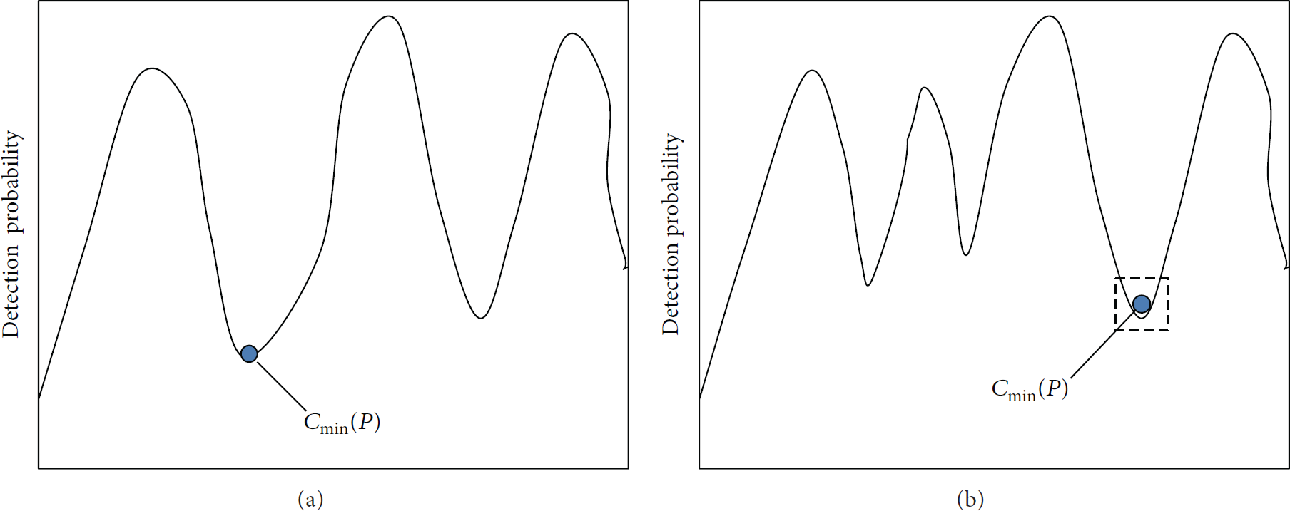
Schematic of joint detection probability. (a) Detection probability before iteration. (b) Detection probability after iteration.

4.2. The Movement of Mobile Nodes

After the termination of iteration, the position of the virtual nodes is defined as coverage vacancies. For the initial network deployment, Firstly we construct a bipartite graph $G=(V,E)$ , $V=V_{\mathrm{1}}\cup V_{\mathrm{2}}$ , where $V_{\mathrm{1}}$ denotes the set of mobile nodes and $V_{\mathrm{2}}$ denotes the set of virtual nodes. We take the moving distance as cost to illustrate the construction method of the bipartite graph. The concrete method is given by the following.

• (1)

Add all the movable nodes into $V_{\mathrm{1}}$ .

(2)

Add all the virtual nodes into $V_{\mathrm{2}}$ .

(3)

For $\forall u\in V_{\mathrm{1}}$ and $\forall \nu \in V_{\mathrm{2}}$ , if mobile node u can reach v, (the distance between u and v does not exceed the maximum moving distance $d_u$ of u or the remaining energy of u is within a certain range $E_{\text{residual}}$ ) then add an edge $(u,v)$ into the bipartite graph; the weight of the edge $(u,v)$ which is defined as $w(u,v)$ denotes the distance between sensor node u and virtual node v, otherwise, $w(u,v)=\mathrm{0}$ .

A set H of independent edges in a graph $G=(V,E)$ is called a matching (see [22]). H is a matching of $U\subseteq V$ if every vertex in U is incident with an edge in H. The vertices in U are then called matched (by H); vertices not incident with any edge of H are unmatched. Because the two ends of any edge of G lie in different set of vertices, the number of edges in H denotes that $|H|$ virtual nodes (that is coverage holes) are covered by $|H|$ mobile nodes. Corresponding cost is given by $C_H={\sum }_{(u,v)}^{}w(u,v)$ . Thus, maximizing the network coverage and minimizing the moving distance in this condition can be transformed into a problem of finding a maximum matching $H_{\text{opt}}$ of bipartite graph G which has a minimum cost, that is, for any matching H of G, $|H|\le |H_{\text{opt}}|$ ; If $|H|=|H_{\text{opt}}|$ , then $C(H)\ge C(H_{\text{opt}})$ . A maximum matching $H_{\text{opt}}$ of bipartite graph G which has a minimum cost represents an optimal mobile solution. Deploying the mobile nodes according to the optimal mobile solution, the coverage of the network can be improved while the moving distance is the smallest.

For illustration, an example is given here. We assume that the vertex set of bipartite graph G is $V=V_1\cup V_2$ . The mobile node set $V_{\mathrm{1}}=\{x_{\mathrm{1}},x_{\mathrm{2}},x_{\mathrm{3}},x_{\mathrm{4}},x_{\mathrm{5}}\}$ , and virtual node set $V_{\mathrm{2}}=\{y_{\mathrm{1}},y_{\mathrm{2}},y_{\mathrm{3}},y_{\mathrm{4}},y_{\mathrm{5}}\}$ . Here, we just consider movement distance. As introduced above, if the distance between $x_i$ and $y_j$ does not exceed the maximum moving distance $d_{x_i}$ of $x_i$ , it indicates that mobile node $x_i$ can reach $y_j$ , then add an edge $(x_i,y_j)$ into the bipartite graph G . The weight of edge $(x_i,y_j)$ is defined as $w(x_i,y_j)$ which denotes the distance between sensor node $x_i$ and virtual node $y_i$ ; otherwise, $w(u,v)=\mathrm{0}$ . Otherwise, add an edge whose weight is 0 into the bipartite graph G. For example, if the distance between $x_1$ and $y_1$ is 3, it is assumed that the maximum moving distance of $x_1$ is 10, then add an edge $(x_1,y_1)$ whose weight is 3 into the bipartite graph G. Similarly, we can obtain the weight of other edges of bipartite G, as shown in Figure 2(a). After the construction of the bipartite graph G, then we can obtain a maximum matching $H_{\text{opt}}$ of bipartite graph G which has a minimum cost $H_{\text{opt}}=\{x_{\mathrm{1}}{y}_{\mathrm{5}},x_{\mathrm{2}}{y}_{\mathrm{3}},x_{\mathrm{3}}{y}_{\mathrm{4}},x_{\mathrm{4}}{y}_{\mathrm{2}},x_{\mathrm{5}}{y}_{\mathrm{1}}\}$ .

Figure 2

An example of bipartite graph construction (a) Weight matrix of edges of bipartite graph (b) the constructed bipartite graph.

According to $H_{\text{opt}}$ , we will move $x_{\mathrm{1}}$ to $y_{\mathrm{5}},x_{\mathrm{3}}$ to $y_{\mathrm{4}},x_{\mathrm{4}}$ to $y_{\mathrm{2}}$ , and $x_{\mathrm{5}}$ to $y_{\mathrm{1}}$ , respectively. For $w(x_{\mathrm{2}},y_{\mathrm{3}})=\mathrm{0}$ , we do not move node $x_{\mathrm{2}}$ . The corresponding cost is 4. The concrete algorithm is as found in Algorithm 1.

Algorithm 1: Algorithm FABGM.

input: Static nodes $S=\left\{s_1,s_2,\dots ,s_N\right\}$ , Mobile nodes $V_1=\left\{v_1,v_2,\dots ,v_M\right\}$ , $E_{\text{residual}}$ , $d_u$ , $u\in V_1$ , $t_{\text{pre}}$ , $P_s$

False-alarm probability parameter $\alpha ,\beta ,\gamma ,\sigma ,e_{\mathrm{tr}}$

Output:

  (1)   $t\leftarrow \mathrm{0}$ .

  (2)  Calculate $C_k\left(P\right)$ of the target at any position k of area $A_s$ using (19).

  (3)  Repeat:

  (4)     Search $C_{\min }(P)$ , construct set of virtual node $V_{\mathrm{2}}$ = $\{\left(x_{E,\mathrm{1}},y_{E,\mathrm{1}}\right),\left(x_{E,2},y_{E,2}\right),\dots ,$

       $\left(x_{E,\mathrm{M}},y_{E,\mathrm{M}}\right)\}$ .

  (5)     Update the static node set $S=\left\{s_{\mathrm{1}},s_{\mathrm{2}},\dots ,s_N\right\}\cup V_{\mathrm{2}}$ .

  (6)     Update iteration times, set t: $t=t+\mathrm{1}$ .

  (7)     Calculate $C_k\left(P\right)$ of the target at any position k of area $A_s$ using (19).

  (8)  Until (iteration time t is larger than $t_{\text{pre}}$ or $C_{\min }(P)$ is larger than $P_s$ )

  (9)     Construct bipartite graph $G=(V,E)$ , calculate $H_{\text{opt}}$ .

  (10)    Adjust the position of the mobile node $v_i,v_i\in V_{\mathrm{1}}$ according to optimal mobile solution

        which is in consistent with $H_{\text{opt}}$ .

5. Simulations Results

Now we present simulation results regarding the proposed algorithm. All of the simulation results given in the following are obtained by programs in C++ and Matlab. We consider a specific WSNs scenario where the field has a square shape of size $\mathrm{80}\times \mathrm{80}$  m²; 60 sensor nodes (including static and mobile nodes) are randomly distributed over this field. We ran 100 simulations for every result and calculated the average result. The experimental parameters are shown in Table 1.

Table 1

Settings of simulation parameter.

Parameter	Value
The area of $A_s$	$\mathrm{80}\times \mathrm{80}$  m2
The iteration times t	30
Total number of nodes: n	60
The value of γ	2
The value of σ	1
The value of β	7
The value of $P_F=\alpha$	5%

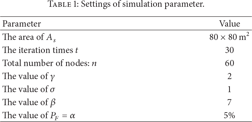
Figure 3 shows the schematic diagram of movement condition of the mobile nodes. The circle represents the mobile node and the five-pointed star represents coverage void. If a circle i and a five-pointed star j are connected by a line, it indicates that mobile node represented by circle i can move to the coverage hole represented by the five-pointed star j. As introduced above, if the distance between mobile node u and coverage hole v exceeds the maximum moving distance $d_u$ of u or the remaining energy of u is less than a preset value $E_{\text{residual}}$ , we set $w(u,v)=\mathrm{0}$ . Thus, according to practical situation, we can set different $d_u$ and $E_{\text{residual}}$ , then we can obtain a different weight matrix regarding edges of the constructed bipartite graph and different optimal mobile solutions. Therefore, the proposed algorithm is more flexible and reflects reality well. After performing FABGM algorithm, the sensors are distributed uniformly in the detection area, which helps to increase the system efficiency, improve energy conservation, and decrease the probability of missing an event.

Figure 3

Position of mobile nodes before and after optimization.

Figure 4 provides the schematic diagram of detection probability distribution comparison between the random method and our deployment method. It is obvious that there are many coverage vacancies and points with low probability in the network after the initial random deployment. From Figure 4(b), we know that the proposed algorithm in this paper can decrease the coverage void and improve the coverage performance of the network. Figure 5 shows the coverage performance of FABGM algorithm when the mobile nodes percentage varies from 0% to 80%. Due to the lack of reference system, we compare the proposed algorithm with the initial deployment. We can see that our deployment can enhance coverage compared to the initial random deployment and that the network coverage quality increases with the number of mobile nodes increase. However, when the mobile node percentage is larger than 50%, network coverage increases slowly along with the increase of the number of mobile nodes.

Figure 4

Distribution of joint detection probabilities. (a) Random deployment. (b) Distribution after running FABGM.

Figure 5

Coverage quality before and after optimization.

In order to analyze the relationship between coverage performance and the value of β, we discuss the network coverage condition when the value of β is 1, 3, 6, and 8 separately. From Figure 6, we know that when the value of β is fixed, the network coverage improves with the increase of number of mobile nodes. When the value of β is small, the network coverage improves apparently. When the value of β is large (e.g., = 6, 8), increasing the number of mobile nodes will not improve network coverage significantly. That is because the value of β is proportionate to $e_{\mathrm{tr}}$ when γ is fixed, when the value of β is large, $e_{\mathrm{tr}}$ is also large. It indicates that each sensor node consumes much energy to transmit signal, so its detection range increases. The initial deployed sensors can almost cover the whole area, and so increasing the number of mobile nodes does not enhance network coverage significantly. The value of β can be determined according to practical application.

Figure 6

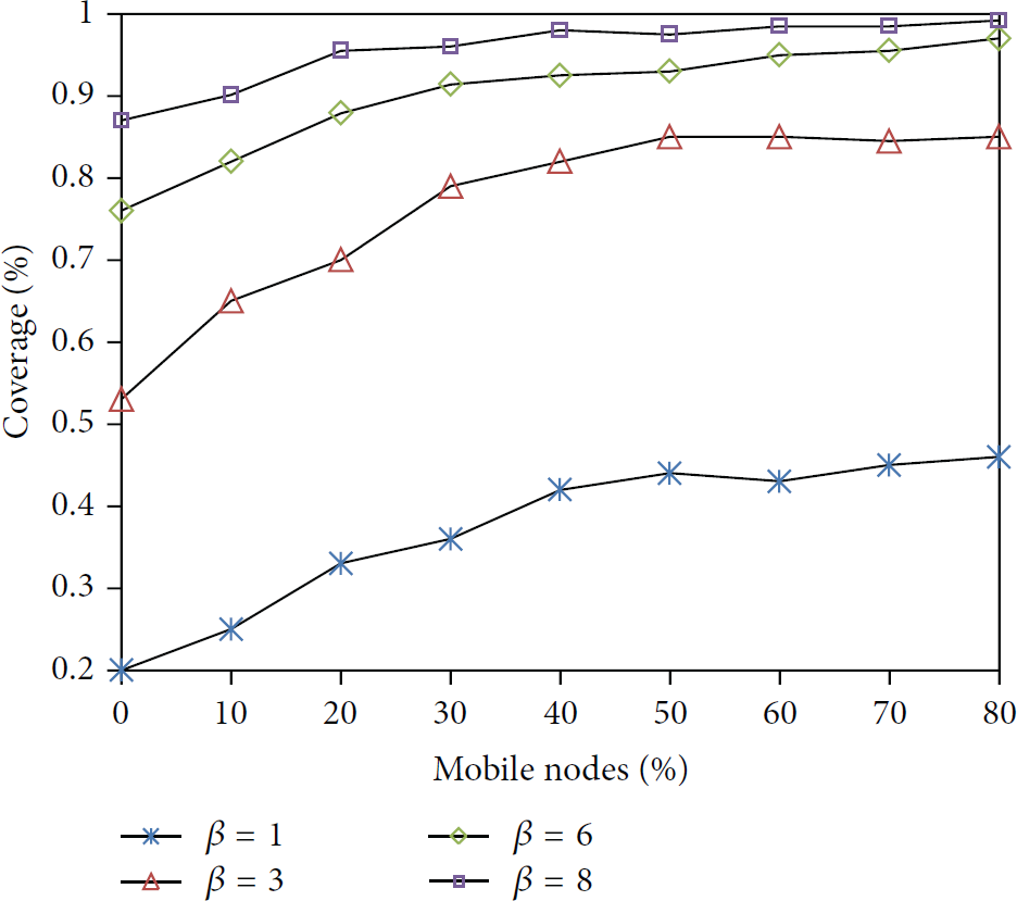
Coverage comparison of different β.

Figure 7 gives the minimum number of sensors required to reach a certain coverage percent when the percentage of mobile sensors varies from 0% to 80%, in 10% increments. As shown in Figure 7, the sensor nodes required in the mixed WSN are less than that in the static WSN. As the percentage of mobile sensors is 40%, the number of sensors in the mixed WSN is about half the number of sensors in the static WSN. The number of sensors needed decrease with the increase of the number of mobile nodes. When the percentage of mobile sensors increases from 0% to 30%, the number of sensors for 80% coverage decreases from 65 to 35, but when the percentage increases from 50% to 70%, the effect is not as significant as before. Considering that the price of mobile sensors is higher than the price of static sensors, it is necessary to determine proper number of mobile nodes in a network. However, the number of mobile nodes is related to the ratio of the price of mobile sensors to the price of static sensors.

Figure 7

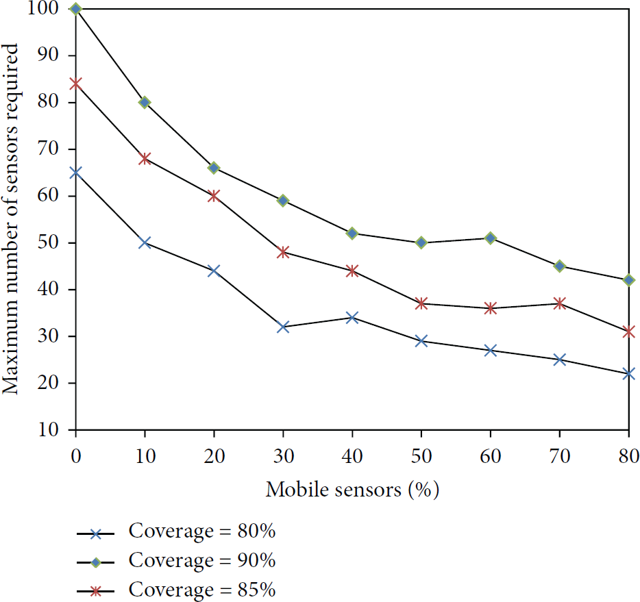
The minimum number of sensors required to reach a coverage percent in different mobile percentages.

Figure 8 shows the cost of WSN to reach 85% coverage at different ratios of the price of mobile sensors to the price of static sensors. When the price discrepancy of mobile nodes and static nodes is minor, increasing the proportion of mobile sensors can reduce the overall cost of WSN. When the ratio is between 2 and 6, the mixed WSN has the lower cost, and also the proportion of mobile sensors is not very high (e.g., 20% ≤ the percentage of mobile sensors ≤ 50%). But when the ratio is greater than 6, it is better that the nodes in the network are all static nodes. It is apparent that the mixed WSN is a best choice when the ratio between the price of the mobile sensor and the price of the static sensor is 2–6. Under this circumstance, our proposed algorithm is useful and can provide a tradeoff between the cost and the coverage.

Figure 8

The cost to reach 85% coverage.

6. Conclusion

Sensor deployment is at the initial stages in sensor networks research. Here, we explore the problem of uncertainty-aware WSNs deployment, and we start with a “random” distribution of the nodes (including mobile nodes and static nodes) over the region of interest. In this paper, we propose a false-alarm deployment algorithm to improve an initial deployment of nodes. After going through the proposed algorithm, the area of interest is covered by uniformly nodes. Simulation results demonstrate the effectiveness of the proposed approach.