Sage Journals: Discover world-class research

Abstract

The mixed wireless sensor networks that are composed of a mixture of mobile and static sensors are the tradeoff between cost and coverage. To provide the required high coverage, the mobile sensors have to move from dense areas to sparse areas. However, where to move and how to move are important issues for mobile sensors. This paper presents a centralized algorithm to assist the movement of mobile sensors. In this algorithm, the management node of the WSN collected the geographical information of all of the static and mobile sensors. Then, the management node executed the algorithm to get the best matches between mobile sensors and coverage holes. Simulation results show the effectiveness of our algorithm, in terms of saving energy and the load balance.

1. Introduction

Wireless sensor networks (WSNs) have been used extensively due to their excellent capability of monitoring real physical environments and collecting data. However, in order to conduct their tasks successfully, it is very important that they be deployed properly, taking into account the limitations of energy support and transmission power.

WSNs cannot be deployed manually in many working environments, such as remote mountainous regions, battlefields, and regions polluted by poisonous gases. An alternative method is scattering the sensors randomly, but this is affected by many uncontrollable factors, and it is difficult to achieve the desired deployment. In early studies, most of the networks consisted of a large number of static nodes, and there were many redundant nodes. Importantly, this approach often led to high cost and uncertainties concerning the coverage.

In the last decade, researchers have focused on mixed networks, which are composed of both static nodes and mobile nodes. Such networks have the advantage of mobility, so they can be moved to appropriate positions to enhance the extent of coverage and reduce the number of nodes. However, there are few algorithms that have been proposed to guide the mobile sensors from their original positions to the desired positions in mixed wireless sensor networks except two classic algorithms which will be introduced in Section 2.

Our problem statement is “given the target area, static sensors that are immobile, and sensors with flexible mobility, design and implement a plan that maximizes the coverage of the sensors, minimizes energy consumption, and results in a balanced energy load.” In this paper, we report the results of our design of a new, centralized algorithm for the placement of mobile sensors in a mixed network to achieve the goals mentioned in the problem statement. The algorithm assists in decision making concerning moving the mobile sensors to fill the holes, where coverage was not provided by any sensor. In order to save energy, we attempted to shorten the total distance that all of the mobile sensors moved. In addition, we made sure that no sensors moved an extremely long distance in order to balance the energy load. The implementation of the algorithm was divided into four stages, that is, (1) the management node of the WSN collected the geographical information of all of the static and mobile sensors; (2) the management node executed the algorithm to determine the best positions to which all of the mobile sensors should move to; (3) the management node issued the resulting locations to the mobile sensors through the network management system (NMS); and (4) the mobile sensors moved to the positions specified by the NMS.

The rest of the paper is organized as follows. Section 2 introduces basic information concerning Delaunay triangulation. The centralized algorithm is presented in Section 3, and its performance is evaluated in Section 4. A summary of the paper is presented in Section 5.

2. Related Work

Many significant achievements have been made in the field of energy-efficient coverage. Due to the characteristics of the nodes that comprise WSNs, there are three types of such networks, that is, (1) static WSNs, in which all the nodes are static; (2) mobile WSNs, in which all the sensors are mobile; and (3) mixed WSNs, in which some of the nodes are static and some are mobile.

The greatest weakness of a static WSN is that there must be significant redundancy among the nodes in order to achieve good coverage. As a result, one of the most important issues to consider in the implementation of a static WSN is energy-efficient coverage (EEC). Many algorithms have been proposed to conserve energy and prolong the network's lifetime [1–5]. Among these algorithms, scheduling methods have been shown to be effective in reducing energy consumption by planning the activities of the devices [6–9].

In mobile WSNs, a fundamental issue is the coverage problem. Many techniques have been developed to deal with this issue, such as coverage pattern-based movement [10–13], virtual force-based movement [14, 15], and grid quorum-based movement [16–19]. The greatest weakness of a mobile WSN is its price, which is significantly greater than the price of a static WSN, because the price of mobile sensors is much greater than the price of static sensors.

A mixed WSN is a tradeoff between a static WSN and a mobile WSN. In most cases, a mixed WSN is the best choice. In a previous work, Voronoi diagrams were used to study methods for estimating the coverage holes in mixed sensor networks [20]. The author proposed a collaborative algorithm (Coven) to determine the location of the mobile sensors for enhancing coverage by estimating the relationship between the area of the coverage hole and the coverage radius of the sensors. However, it is not feasible to apply Voronoi diagrams in WSNs due to their excessive complexity.

Concerning the strategy for moving the sensors, one study [21] proposed a bidding protocol in mixed sensor networks that treated static nodes as bidders or consumers and mobile nodes as service providers. An optimal relay placement for indoor sensor networks was proposed. Mobile nodes have a base price which is the size of coverage holes produced by mobile nodes leaving their positions to cover other holes. Static nodes bid for mobile nodes, and the bid price is the size of the coverage holes detected by static nodes. When the bid price for the mobile nodes is less than the price of the static nodes, the mobile nodes will provide service for the static nodes to cover the holes that have been detected by the static nodes. However, the authors provided no discussion of the energy balances of all of the sensors, so the lifetime of the WSN was short. Additionally, applying the bidding protocols in [21], several sensors may have to move a long distance, which would take more time to complete the construction of the sensor network.

In order to improve the effectiveness of the algorithm in paper [21], paper [22] introduced a proxy-based bidding protocol, which was an improvement over the basic bidding protocol. To reduce distances that the mobile sensors had to move, the proxy-based bidding protocol proposes that mobile sensors perform virtual movements from small holes to large holes and that they only perform physical movements after the final destinations have been identified.

To our knowledge, the paper [21] is the first paper on deploying a mixture of static and mobile sensors to meet the coverage requirement, and [22] is an improvement of [21]. There are few other papers that focus on this problem, and we will compare the algorithm in this paper with the two algorithms.

3. Preliminaries

3.1. Assumptions

In our research, we used the classical Boolean sensing model, in which the sensing area is represented by a circle with a radius. The Boolean sensing model facilitated the analysis and helped us understand the problem. Obviously, we must know the locations of all the sensors, and it had been proved that each node in the wireless sensor network had the ability to establish its location through GPS system or some other form of localization technique [23–27]. In our research, we assumed that at least one of the techniques was available in our WSN.

After executing our algorithm, the management node identified the best positions to which all the mobile nodes should move. But we were unable to plan the path from the current position to the desired destination for the mobile nodes. However, there are also several existing techniques that can be used to plan the path, and we assumed that at least one of them was available.

3.2. Preliminary Technique: Delaunay Triangulation

A Voronoi diagram represents the proximity information about a set of nodes. It provides a geometric construction that detects the coverage holes very effectively, especially in distributed algorithms in which position information for all of the sensors is unknown. However, it is not the best choice for centralized algorithms, so we used Delaunay triangulation instead of a Voronoi diagram.

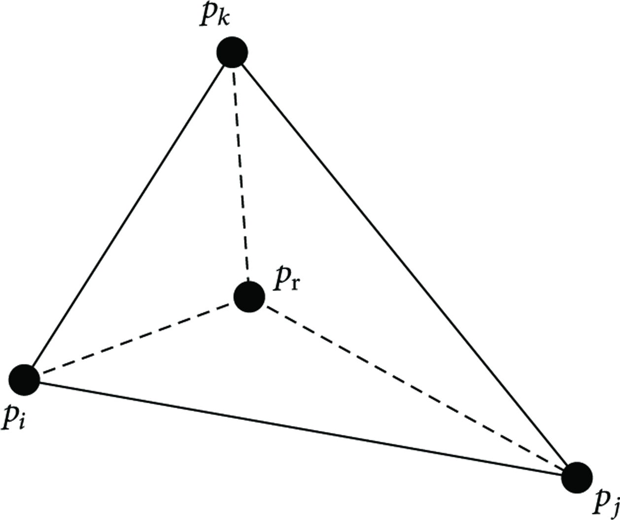
Delaunay triangulation and the Voronoi diagram are dual constructions. Given a set of nodes, we used a randomized incremental algorithm to triangulate them into many triangles, and the circumcenters of the triangles were the key areas that we had to detect carefully. First, we triangulated all of the static nodes and determined the best position for the mobile sensor to provide the desired coverage. Then, the mobile sensor was not moved to any other place, so, in effect, it became a static sensor, and we added it to the set of static nodes. We iterated the process until all of the mobile nodes became static nodes. Then, we determined all of the desired positions for the mobile sensors. The features of Delaunay triangulation guarantee that the distance between the circumcenter of a triangle and its vertices is shorter than the distance between the circumcenter and any other nodes. So, if a the circumcenter of a triangle is not covered by its vertexes, there must be a coverage hole that a mobile sensor should be moved to cover. We will give a detailed introduction in Section 4.

4. Centralized Algorithm

In this section, we present the centralized algorithm, which is divided into four stages. The second stage is the core of the algorithm, and we focused mainly on it. The discussion of the algorithm is presented in four steps, that is, (1) detect the coverage holes, (2) choose the desired positions, (3) use the greedy algorithm to obtain an initial result, and (4) optimize the initial result using the 2-exchange optimization algorithm.

4.1. Detect the Coverage Holes

We used Delaunay triangulation to detect the coverage holes. First, we triangulated the set of static nodes into many triangles and calculated the circumcenter of every triangle, as shown in Figure 1. Second, we detected whether the circumcenter was covered by the three static sensors that formed the triangle. If the circumcenter was covered, it is not a coverage hole. The size of the hole was calculated as

\begin{matrix} s = π * {(d - R_{s})}^{2}, d \geq R_{s}, \end{matrix}

(1)

where d is the distance between the circumcenter and the vertexes of the triangle and

R_{s}

is the sensing range of the sensor, as shown in Figure 2. Because π and

R_{s}

are constants for a WSN, we can use d to represent the size of the coverage hole. If

d \leq R_{s}

, there is no coverage hole; if

d \geq R_{s}

and

d \leq {2 R}_{s}

, there is a hole, most of which can be covered by one mobile sensor; if

d \geq {2 R}_{s}

, there is a big hole that may require more than one mobile node to cover it completely.

Figure 1

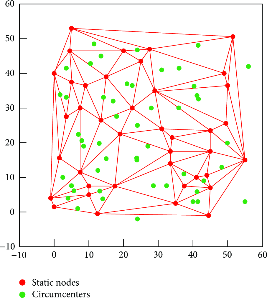
Delaunay triangulation.

Figure 2

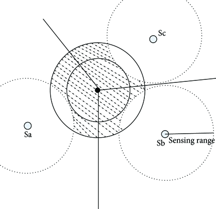
Size of a coverage hole.

4.2. Choose the Desired Positions

Having detected the holes, we must decide which hole is to be covered by a mobile sensor first. To do this, we used the encroaching principle, that is, that the holes adjoining the covered area should be covered preferentially, rather than the bigger holes as has been classically done. The rationale was that if we covered the bigger holes first, there will be locations between the hole and the covered area that will be covered twice. Simulation showed that our approach was better than following the classic approach, as indicated by the improved coverage percentages shown in Figures 3(b) and 3(c), respectively. We calculated the coverage percentage by image processing and determined that the initial coverage percentage was 68.3%, while the coverage percentage of the classic approach was 93.2%, and the coverage percent of the encroaching principle that we used was 95.1%.

Figure 3

The coverage results by different principles.

Our discussion of the randomized incremental algorithm follows. After we had triangulated the set of static nodes, we were able to detect the coverage holes and identify the place the mobile sensors should cover first. Then, we moved one mobile sensor to that place, and the sensor remained stationary after that. Thus, the mobile sensor became a static sensor, resulting in a change in the triangulation of the static sensors. Before we chose the next hole to be covered, we had to obtain the new triangulation and then decide the hole using the encroaching principle. We iterated the process until the coverage percentage reached a constant value, for example, 95%. But we did not have to calculate the new triangulation repeatedly. We can calculate the new triangulation based on the previous result, and this is the core idea of the randomized incremental algorithm.

A triangulation is shown in Figure 4. We added a new point, $p_{r}$ , to the set of nodes and calculated the new triangulation. As shown in Figure 4(b), the new triangulation is only different from the previous triangulation in part. When the number of nodes is large, the difference between the two triangulations is very small, so we just have to calculate a part of the new triangulation. Before we introduce the algorithm, the illegal edge is defined as follows.

Figure 4

A triangulation in randomized incremental algorithm.

In Figure 5(a), there are six angles, that is, ${α_{1}, α_{2}, α_{3}, α_{4}, α_{5}, α_{6}}$ , and there are six angles, that is, ${α_{1}^{'}$ , $α_{2}^{'}$ , $α_{3}^{'}$ , $α_{4}^{'}$ , $α_{5}^{'}$ , $α_{6}^{'}}$ , in Figure 5(b). If $\min (α_{i}) < \min (α_{i}^{'})$ , $1 \leq i \leq 6$ , then $p_{i} p_{j}$ is an illegal edge.

Figure 5

Edge flip.

Figure 6

$p_{r}$ is located in $p_{i} p_{j} p_{k}$ .

Figure 7

$p_{r}$ is located on the edge.

We assumed that T is the triangulation, and the randomized incremental algorithm is described in Algorithm 1.

Algorithm 1

(1) do (add $p_{r}$ to T)

(2) find the triangle $p_{i} p_{j} p_{k} \in T$ that $p_{r}$ in it

(3) if ( $p_{r}$ is located in $p_{i} p_{j} p_{k}$ )

(4) then line $p_{r}$ and the three vertexes of $p_{i} p_{j} p_{k}$ as shown in Figure 6

(5) LegalizeEdge ( $p_{r}$ , $p_{i} p_{j}$ , T);

(6) LegalizeEdge ( $p_{r}$ , $p_{j} p_{k}$ , T);

(7) LegalizeEdge ( $p_{r}$ , $p_{k} p_{i}$ , T);

(8) else ( ${}^{*}{p_{r}}$ is located on the edge, we assume that the edge is $p_{i} p_{j}$ )

(9) line $p_{r}$ and $p_{k}$ , $p_{l}$ as shown in Figure 7

(10) LegalizeEdge ( $p_{r}$ , $p_{i} p_{j}$ , T);

(11) LegalizeEdge ( $p_{r}$ , $p_{j} p_{k}$ , T);

(12) LegalizeEdge ( $p_{r}$ , $p_{k} p_{j}$ , T);

(13) LegalizeEdge ( $p_{r}$ , $p_{j} p_{i}$ , T);

(14) return (T);

The function of LegalizeEdge ( $p_{r}$ , $p_{i} p_{j}$ , T) is describe in Algorithm 2.

Algorithm 2

(1) If ( $p_{i} p_{j}$ is illegal)

(2) then assume $p_{i} p_{j} p_{k}$ is the triangle that adjacent to $p_{i} p_{j} p_{r}$

(3) replace the edge $p_{i} p_{j}$ by $p_{r} p_{k}$

(4) LegalizeEdge ( $p_{r}$ , $p_{i} p_{k}$ , T)

(5) LegalizeEdge ( $p_{r}$ , $p_{j} p_{k}$ , T)

(6) end

Now, we have detected the coverage holes and chosen the desired position successfully, which provides the basis for the next step. The numbers of mobile nodes and desired positions are fixed. Once the mobile nodes have moved to the desired positions, the coverage percentage obviously will be improved. In order to save energy and balance the energy load, we designed a detailed scheme for determining the positions to which the mobile sensors should move. We can describe the problem in mathematical language as follows.

Given two sets of $X$ and Y:

\begin{matrix} X = {x_{1}, x_{2}, \dots, x_{m}}, \\ Y = {y_{1}, y_{2}, \dots, y_{m}}, \end{matrix}

(2)

where m is a constant number. There are no common elements in the two sets, that is,

\begin{matrix} X \cap Y = \emptyset . \end{matrix}

(3)

We must match the elements in X and the elements in Y one to one. For example,

\begin{matrix} {{x_{1}, y_{1}}, {x_{2}, y_{2}}, \dots, {x_{m}, y_{m}}} \end{matrix}

(4)

is a one-to-one match. Also, there is a weight for every match

{x_{i}, y_{j}}

, and we must find a match with the low total weight and without extremely large weight. A heuristic algorithm is a good solution, and we used the greedy algorithm and the 2-exchange optimal algorithm to solve this problem.

In our WSN, the weight of a match is the Euclidean distance between mobiles sensors and the holes that should be covered by the mobile sensors. In order to save energy, mobile nodes should move the shortest distance possible, and, in order to balance the load, the distances should be similar. We assumed two measures for our algorithm, that is, the average distance that the mobile sensors moved and the variance between the distances.

4.3. Obtain an Initial Result by Greedy Algorithm

Now, we have obtained the current positions of the mobile sensors and the positions to which they should move, as shown in Figure 8. For example, the red stars are mobile sensors, and the green points are the coverage holes. We determined the acceptable match in the following two steps, that is, (1) obtain an initial result by greedy algorithm and (2) optimize the result using the 2-exchange optimization algorithm.

Figure 8

The initial situation.

Now, we introduce the greedy algorithm in five steps.

Algorithm 1.

Greedy algorithm for match

Input. $2 n$ points, n mobile sensors, and n coverage holes.

Output. one-to-one match for mobile sensors and holes.

Step 1.

We order the holes from 1 to n as shown in Figure 9, where n is the number of the holes.

Figure 9

The match result by greedy algorithm.

Step 2.

Push the geographical information of the holes to a stack in reverse order and push the information of mobile nodes in another stack randomly, as shown in Figure 10.

Figure 10

(a) and (c) are the initial trace, and (b) and (d) are the trace that have been optimized.

Step 3.

Choose the mobile node in stack M that is the closest to the hole in the top of stack H and record the match.

Step 4.

Pop stack H and delete the mobile node in stack M.

Step 5.

If there are no holes in stack H, exit the algorithm, otherwise, return to Step 3.

The results of the algorithm are shown in Figure 9. Every line segment with an arrow indicates that a mobile sensor should move to a coverage hole. It cannot meet our requirements for both average distance and the variance of the distance, and we had to improve the results by using the 2-exchange optimal algorithm.

As shown in Figure 9, when the serial number of the hole is smaller, it is more likely that the length of the line segment with an arrow that points to the hole from the corresponding mobile sensor is shorter. It is an inherent flaw of the greedy algorithm that the results are optimal in local but are not as good in global.

4.4. Optimize the Initial Result by Using the 2-Exchange Optimization Algorithm

The results shown in Figure 9 are not good enough, and we optimized the results by using the 2-exchange optimization algorithm. There is no common point for any two lines because the mobile nodes and coverage holes are a one-toone match. The core idea of the algorithm is to exchange the destination of any two line segments to see whether their total length decreased. If so, we exchanged the destination of the line segment and recorded the result; otherwise, we maintained the present status. The 2-exchange optimization algorithm is a special case of the N-exchange optimal algorithm, and, if N is equal to the number of mobile sensors, the result is the best result.

One problem is the organization of the exchange order to guarantee that no line is ignored or repeated. Because the holes match the lines one to one, the number of a hole can represent the corresponding line, that is to say, the lines are ordered from 1 to n. The optimization algorithm is described in Algorithm 3.

Algorithm 3: 2-exchange optimization algorithm.

Input: n lines with total length of L

Output: n lines with total length of $L^{''} < L$ and the variance of $L^{'} <$ the variance of L

$L^{''} = L$ ;

(1) do {

(2) for $i = 1$ : $n - 1$

(3) for $j = i + 1$ : n

(4) exchange the destination of line i and line j;

(5) if (the total length of the two lines decreased)

(6) record the result;

(7) else

(8) maintain the present status;

(9) end

(10) end

(11) $L^{'} = L^{''}$ ;

(12) $L^{''}$ = the total length of n new lines;

(13) } while ( $L^{'} - L^{''} > ε$ );

where $ε$ is a threshold, it represent the precision of the result we got.

The main part of the algorithm is a loop, and, from the results of the simulation, we found that the margin of improvement in the first loop was the most obvious; the more times we executed the loop, the less improvement we obtained from every execution. Though it is a heuristic algorithm, its complexity cannot be ignored. 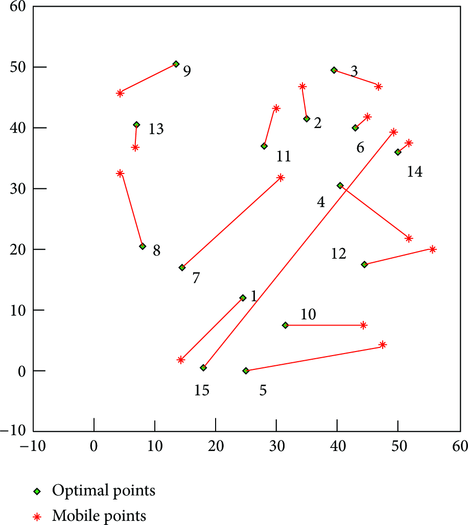In fact, if we insist on finding the 2 best results, that is to say, we execute the loop until $L^{'} - L^{''} = 0$ , it is likely that the time required would be unacceptable. In addition, in a WSN, an acceptable result that can be obtained in a simple way is the best result. In fact, the result we obtained was excellent, just 1.04–1.06 times the best match obtained mathematically, and the complexity was reduced significantly.

Figures 10(a) and 10(c) are the initial trace, and Figures 10(b) and 10(d) are the trace after the optimization.

When there were 15 mobile sensors and $ε = 5$ meters, the loop was executed 2-3 times, and the convergence property was excellent, as shown in Figure 10(c). In order to test the pressure resistance of the algorithm, we assumed that there were 100 mobile sensors and that the loop was executed four times, as shown in Figure 10(d). It is apparent that the complexity increased slowly as the number of mobile sensors increased.

5. Performance Evaluations

5.1. Tradeoff between Cost and Coverage

Before we tested the effectiveness of our algorithm, first, we proved that the mixed WSN was meaningful in real applications. The cost of a WSN is based on the cost of the sensors. We ran simulations for three different compositions of sensors in a WSN and set the coverage to be 90%, 95%, and 98%, respectively. We assumed that the target area was a 50-m × 50-m, square, flat, field and randomly scattered 60 sensors, including static sensors and mobile sensors, in the field. The percentage of mobile sensors varied from 0% to 100%, in 10% increments. The transmission range was set as 20 m, and the sensing range was set as 5 m. We ran 100 simulations for every result and calculated the average result.

There were three cases of network compositions, that is, (1) all sensors were static and random deployment was used; (2) all sensors were mobile, and the VOR protocol was used to deploy the sensors; and (3) for sensor deployment, a percentage of the sensors were mobile, and we used our centralized algorithm. The results are shown in Figure 11.

Figure 11

The minimum number of sensors required to reach a coverage percent in different mobile percentage.

Because of the randomness of the static sensors, sometimes we could not calculate the accurate minimum number of the sensors to reach a certain coverage. For example, if all the sensors were static and, unfortunately, we placed them all at the same position, we could never cover the target field. In this paper, we scattered the same number sensors 100 times and obtained 100% coverage in each case. For a number of sensors, N, if the average coverage just reached a certain coverage, such as 95% and for $N - 1$ , the average coverage cannot reach 95%, then we defined the number N as the minimum number of sensors required to reach a coverage of 95%.

As shown in Figure 11, in the static WSN, the most sensors were required; in the mobile WSN, the least sensors were required; in the mixed WSN, the number of sensors required was between the number required for the static WSN and the number required for the mobile WSN. Obviously, the mixed WSN significantly reduced the number of sensors compared to the static WSN. When the percentage of mobile sensors was 30%, the number of sensors in the mixed WSN was about half of the number of sensors in the static WSN, and as the proportion of mobile sensors increased, the number of sensors needed decreased. The number of sensors required in a mobile WSN was less than the numbers required by static or mixed WSNs. But as the number of mobile sensors incraesed, the marginal effect decreased; fore example, when the percentage of mobile sensors increased from 0% to 10%, the number of sensors for 98% coverage decreased from 120 to 85, but when the percentage incraesed from 50% to 60%, the effect was not as significant as before. In addition, the price of mobile sensors is higher than the price of static sendors; thus, determing which WSN is the cheapest is related to the ratio of the price of mobile sensors to the price of static sensors. In conclusion, none of the three types of WSN is always the best in any situation.

Figure 12 shows the costs of these three types of WSN to reach 95% coverage. Based on different price ratios of mobile sensors to static sensors, the overall cost of a WSN can be somewhat different. When the ratio is low (e.g., ≤1.5), increasing the percentage of mobile sensors can reduce the overall cost, and the mobile WSN is the best choice. When the ratio is higher (e.g., 2 ≤ the ratio ≤ 7), the mixed WSN has the lowest cost, and the percentage of mobile sensors is not very high (e.g., 10% ≤ the percentage of mobile sensors ≤ 50%). But if the mobile sensor is much more expensive (e.g., the ratio > 7), the static WSN is the best choice.

Figure 12

The cost of sensors to reach 95% coverage.

If the ratio between the price of the mobile sensor and the price of the static sensor is 2–7, the mixed WSN is a good choice. Under this circumstance, our centralized algorithm is useful, and the result is a balance between the cost and the coverage.

5.2. Coverage

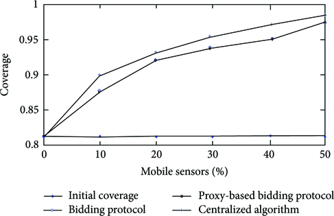
The bidding protocol and the proxy-based bidding protocol are two classic protocols in redeploying mobile sensors in a mixed WSN, and we compared our results to the results of these protocols. From Section 5.1, we know that, most of the time, the percentage of mobile sensors cannot be greater than 50%, so we only considered these situations.

As shown in Figure 13, the mixed WSN can improve the coverage significantly; if the WSN is static, the coverage percentage is about 80% and the mixed WSN is about 90 to 98%. In terms of coverage, there is no preference between the bidding protocol and the proxy-based bidding protocol. In our centralized algorithm, the coverage was higher than it was in the bidding protocols. In fact, the bidding protocols provided the same coverage as the greedy algorithm, and our encroaching principle was better than the greedy algorithm.

Figure 13

Coverage by different algorithms.

5.3. Energy Efficiency

Our algorithm is centralized, and it is executed in the management node. After the algorithm has terminated, the management node will issue the result to the mobile nodes only once, and the mobile nodes will move to the proper position to improve the coverage. We should notice that the management node is not strictly energy limited, and there are few communications between the nodes in the WSN. So, the total energy consumption is just associated with mechanical movement, and we used the average distance that the sensors were moved to determine the energy consumption.

Figure 14 shows the average distance that the sensors were moved in the three protocols. It is apparent that the average distance of basic bidding protocol is the longest and that the result of the centralized algorithm is the best. Obviously, the reason is that the nodes in the distributed algorithm just have part of the geographical information of all the nodes and the management node has all the geography information of all of sensors. Because it has more information, the centralized algorithm produced good results, and it is a global optimization. Conversely, the results of the distributed algorithm were not very good because it had less information, and the results comprised only a partial optimization. Compared with basic-bidding protocol, the results of the proxy-based protocol were better.

Figure 14

Average moving distance.

In the distributed algorithm, the total energy consumption is comprised of two parts, that is, mechanical movement and communication. It is evident from Figure 14 that the total energy consumption of the centralized algorithm is less than just the mechanical movement in the distributed algorithm, so it is considerably less than the sum of the two parts.

Thus, our protocol is much more energy efficient than the two distributed protocols, that is, the basic bidding protocol and the proxy-based bidding protocol.

5.4. Load Balance

To show the results more clearly, we increased the number of mobile sensors to 100 and generated 100 coverage holes randomly. Then, we matched them using the centralized algorithm and gathered statistics related to the distances that the sensors were moved. We used the variance of the 100 distances to measure the load balance. The smaller the variance, the more balanced the load is.

As shown in Figure 15 for the centralized algorithm, most of the distances that the mobile sensors were moved were between zero and 30 m, and the distances were more concentrated than they were in the other two protocols. The variance of the distances for the centralized algorithm was 13.38, which was smaller than 78.25, the variance of the proxy-based bidding protocol, and 127.34, the variance of the basic bidding protocol. The centralized algorithm performed very well for load balancing, and it prolonged the lifetime of the WSN.

Figure 15

Statistic of the moving distance for the three protocols.

6. Conclusions and Future Work

In this paper, we proposed a novel, centralized algorithm to deploy a mixture of mobile and static sensors to construct sensor networks to provide the required uniform sensing service in harsh environments. We used Delaunay triangulation rather than a Voronoi diagram to detect the coverage holes, because it was easier and provided equivalent results. Our performance evaluation showed that for the same conditions, the centralized algorithm was better than the distributed algorithm in coverage percentage, energy-efficiency, and load balancing. Also, we found that it can prolong the lifetime of the WSN significantly because of the energy efficiency and load balance. The reason of the centralized algorithm being better than the distributed algorithm was that it has the overall topology of the WSN, which, in theory, allows us to obtain the global optimum solution.

As future work, we will improve the algorithm in two ways, that is, (1) in order to improve the precision of the coverage, we plan to introduce the probabilistic disk model which is more accurate instead of the classical Boolean sensing model and (2) to further improve the performance of our matching algorithm which is the core of this paper; we plan to introduce some models in Graph Theory and Operations Research Theory.

Footnotes

Acknowledgments

This research is supported by National Natural Science Foundation of China under Grant 61071076, the Academic Discipline and Postgraduate Education Project of Beijing Municipal Commission of Education, National High-tech Research and Development Plans (863 Program) under Grant 2011AA010104-2.

References

Heo

Hong

Cho

EARQ: energy aware routing for real-time and reliable communication in wireless industrial sensor networks

IEEE Transactions on Industrial Informatics 2009 5 1 3 11

2-s2.0-62449084821

10.1109/TII.2008.2011052

Cui

Zhang

Fan

A low energy intelligent clustering protocol for wireless sensor networks

Proceedings of the IEEE International Conference on Industrial Technology (ICIT '10)

March 2010

1675 1682

10.1109/ICIT.2010.5472629

Luntovskyy

Vasyutynskyy

Kabitzsch

Propagation modeling and placement algorithms for wireless sensor networks

Proceedings of the IEEE International Symposium on Industrial Electronics (ISIE '10)

July 2010

Bari, Italy

3493 3497

2-s2.0-78650397040

10.1109/ISIE.2010.5637393

Nouh

Abbass

R. A.

Seoud

D. A. E.

Ali

N. A.

Daoud

R. M.

Amer

H. H.

ElSayed

H. M.

Effect of node distributions on lifetime of Wireless Sensor Networks

Proceedings of the IEEE International Symposium on Industrial Electronics (ISIE '10)

July 2010

Bari, Italy

434 439

2-s2.0-78650338676

10.1109/ISIE.2010.5637472

Zhao

Y. Z.

Nguyen

T. N.

Miao

An energy-efficient MAC protocol with adaptive scheduling for wireless sensor networks

Proceedings of the 7th IEEE International Conference on Industrial Informatics (INDIN '09)

June 2009

446 451

10.1109/INDIN.2009.5195845

Lin

Zhang

An ant-colony-system-based activity scheduling method for the lifetime maximization of heterogeneous wireless sensor networks

Proceedings of the 12th Annual Conference on Genetic and Evolutionary Computation

July 2010

23 30

10.1145/1830483.1830488

Chen

Sun

Chen

H. H.

Energy-efficient coverage based on probabilistic sensing model in wireless sensor networks

IEEE Communications Letters 2010 14 9 833 835

Jia

Chen

Chang

Tan

Energy efficient coverage control in wireless sensor networks based on multi-objective genetic algorithm

Computers & Mathematics with Applications 2009 57 11-12 1756 1766

Lin

X. M.

Zhang

Liu

H. L.

Optimal node scheduling for the lifetime maximization of two-tier wireless sensor networks

Proceedings of the IEEE Congress on Evolutionary Computation

July 2010

1 8

10.1109/CEC.2010.5586264

10.

Wang

P. C.

Hou

T. W.

Yan

R. H.

Maintaining coverage by progressive crystal-lattice permutation in mobile wireless sensor networks

Proceedings of the 2nd IEEE International Conference on Systems and Networks Communications (ICSNC '06)

November 2006

Tahiti, Polynesia

1 6

2-s2.0-40249115090

10.1109/ICSNC.2006.53

11.

Heo

Varshney

P. K.

Energy-efficient deployment of intelligent mobile sensor networks

IEEE Transactions on Systems, Man, and Cybernetics A 2005 35 1 78 92

2-s2.0-11844258234

10.1109/TSMCA.2004.838486

12.

Wang

Y. C.

C. C.

Tseng

Y. C.

Efficient placement and dispatch of sensors in a wireless sensor network

IEEE Transactions on Mobile Computing 2008 7 2 262 274

2-s2.0-37549044736

10.1109/TMC.2007.70708

13.

Wang

Y. C.

Tseng

Y. C.

Distributed deployment schemes for mobile wireless sensor networks to ensure multilevel coverage

IEEE Transactions on Parallel and Distributed Systems 2008 19 9 1280 1294

2-s2.0-49349106443

10.1109/TPDS.2007.70808

14.

Zou

Chakrabarty

Sensor deployment and target localization in distributed sensor networks

ACM Transactions on Embedded Computing Systems 2004 3 1 61 91

15.

Howard

Mataric

M. J.

Sukhatme

G. S.

Mobile sensor network deployment using potential fields: a distributed, scalable solution to the area coverage problem

Proceedings of the 6th International Symposium on Distributed Autonomous Robotic System (DARS '02)

2002

1 10

16.

Chellappan

Bai

Xuan

Mobility limited flip-based sensor networks deployment

IEEE Transactions on Parallel and Distributed Systems 2007 18 2 199 211

2-s2.0-33846863593

10.1109/TPDS.2007.28

17.

Chellappan

Bai

Xuan

Zhang

Deploying wireless sensor networks under limited mobility constraints

IEEE Transactions on Mobile Computing 2007 6 10 1142 1157

2-s2.0-34548327168

10.1109/TMC.2007.1032

18.

Jiang

Kline

Krantz

Mobility control for complete coverage in wireless sensor networks

Proceedings of the 28th International Conference on Distributed Computing Systems Workshops (ICDCS '08)

June 2008

Beijing, China

291 296

2-s2.0-51849106086

10.1109/ICDCS.Workshops.2008.18

19.

Yang

Dai

Localized movement-assisted sensor deployment in wireless sensor networks

Proceedings of the IEEE International Conference on Mobile Ad Hoc and Sensor Sysetems (MASS '06)

October 2006

Vancouver, Canada

753 758

2-s2.0-39049095779

10.1109/MOBHOC.2006.278646

20.

Ghosh

Estimating coverage holes and enhancing coverage in mixed sensor networks

Proceedings of the 29th Annual IEEE International Conference on Local Computer Networks (LCN '04)

November 2004

68 76

2-s2.0-20544442644

10.1109/LCN.2004.53

21.

Wang

Cao

La Porta

T. F.

A Bidding protocol for deploying mobile sensors

Proceedings of the 11th IEEE International Conference on Network Protocols (ICNP '03)

November 2003

22.

Wang

Cao

Berman

La Porta

T. F.

Bidding protocols for deploying mobile sensors

IEEE Transactions on Mobile Computing 2007 6 5 515 528

2-s2.0-33947622591

10.1109/TMC.2007.1022

23.

Dommety

Jain

Potential networking applications of global positioning systems (GPS)

1996 TR-24

Department of Computer Science and Engineering, Ohio State University

24.

Kaplan

E. D.

Understanding GPS: Principles and Applications 1996

Artech House

25.

Huang

Blum

Stankovic

Abdelzaher

Range-free localization schemes for large scale sensor networks

Proceedings of the 9th Annual International Conference on Mobile Computing and Networking (MobiCom '03)

September 2003

81 95

10.1145/938985.938995

26.

Evans

Localization for mobile sensor networks

Proceedings of the 10th Annual International Conference on Mobile Computing and Networking (MobiCom '04)

September 2004

45 57

10.1145/1023720.1023726

27.

Ssu

K. F.

C. H.

Jiau

H. C.

Localization with mobile anchor points in wireless sensor networks

IEEE Transactions on Vehicular Technology 2005 54 3 1187 1197

2-s2.0-21244474042

10.1109/TVT.2005.844642

An Energy-Efficient Motion Strategy for Mobile Sensors in Mixed Wireless Sensor Networks

Abstract

1. Introduction

2. Related Work

3. Preliminaries

3.1. Assumptions

3.2. Preliminary Technique: Delaunay Triangulation

4. Centralized Algorithm

4.1. Detect the Coverage Holes

4.2. Choose the Desired Positions

Algorithm 1

Algorithm 2

4.3. Obtain an Initial Result by Greedy Algorithm

Algorithm 1.

Step 1.

Step 2.

Step 3.

Step 4.

Step 5.

4.4. Optimize the Initial Result by Using the 2-Exchange Optimization Algorithm

Algorithm 3: 2-exchange optimization algorithm.

5. Performance Evaluations

5.1. Tradeoff between Cost and Coverage

5.2. Coverage

5.3. Energy Efficiency

5.4. Load Balance

6. Conclusions and Future Work

Footnotes

Acknowledgments

References